POWER SPECTRA OF RANDOM SPIKES AND RELATED COMPLEX SIGNALS, WITH APPLICATION TO COMMUNICATIONS

合集下载

The_Spectral_Analysis_of_Random_Signals

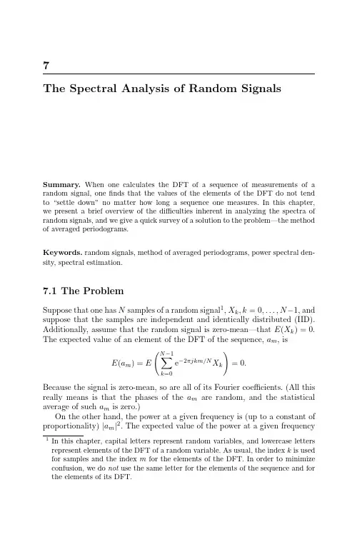
7The Spectral Analysis of Random Signals Summary.When one calculates the DFT of a sequence of measurements of a random signal,oneﬁnds that the values of the elements of the DFT do not tend to“settle down”no matter how long a sequence one measures.In this chapter, we present a brief overview of the diﬃculties inherent in analyzing the spectra of random signals,and we give a quick survey of a solution to the problem—the method of averaged periodograms.Keywords.random signals,method of averaged periodograms,power spectral den-sity,spectral estimation.7.1The ProblemSuppose that one has N samples of a random signal1,X k,k=0,...,N−1,and suppose that the samples are independent and identically distributed(IID). Additionally,assume that the random signal is zero-mean—that E(X k)=0. The expected value of an element of the DFT of the sequence,a m,isE(a m)=EN−1k=0e−2πjkm/N X k=0.Because the signal is zero-mean,so are all of its Fourier coeﬃcients.(All this really means is that the phases of the a m are random,and the statistical average of such a m is zero.)On the other hand,the power at a given frequency is(up to a constant of proportionality)|a m|2.The expected value of the power at a given frequency 1In this chapter,capital letters represent random variables,and lowercase letters represent elements of the DFT of a random variable.As usual,the index k is used for samples and the index m for the elements of the DFT.In order to minimize confusion,we do not use the same letter for the elements of the sequence and for the elements of its DFT.587The Spectral Analysis of Random Signalsis E(|a m|2)and is non-negative.If one measures the value of|a m|2for some set of measurements,one is measuring the value of a random variable whose expected value is equal to the item of interest.One would expect that the larger N was,the more certainly one would be able to say that the measured value of|a m|2is near the theoretical expected value.One would be mistaken.To see why,consider a0.We know thata0=X0+···+X N−1.Assuming that the X k are real,weﬁnd that|a0|2=N−1n=0N−1k=0X n X k=N−1n=0X2k+N−1n=0N−1,k=nk=0X n X k.Because the X k are independent,zero-mean random variables,we know that if n=k,then E(X n X k)=0.Thus,we see that the expected value of|a0|2isE(|a0|2)=NE(X2k).(7.1) We would like to examine the variance of|a0|2.First,consider E(|a0|4). Weﬁnd thatE(|a0|4)=NE(X4i)+3N(N−1)E2(X2i).(See Exercise5for a proof of this result.)Thus,the variance of the measure-ment isE(|a0|4)−E2(|a0|2)=NE(X4i)+2N2E2(X2i)−3NE2(X2i)=Nσ2X2+2(N2−N)E2(X2i).Clearly,the variance of|a0|2is O(N2),and the standard deviation of|a0|2is O(N).That is,the standard deviation is of the same order as the measure-ment.This shows that taking larger values of N—taking more measurements—does not do much to reduce the uncertainty in our measurement of|a0|2.In fact,this problem exists for all the a m,and it is also a problem when the measured values,X k,are not IID random variables.7.2The SolutionWe have seen that the standard deviation of our measurement is of the same order as the expected value of the measurement.Suppose that rather than taking one long measurement,one takes many smaller measurements.If the measurements are independent and one then averages the measurements,then the variance of the average will decrease with the number of measurements while the expected value will remain the same.Given a sequence of samples of a random signal,{X0,...,X N−1},deﬁne the periodograms,P m,associated with the sequence by7.3Warm-up Experiment59P m≡1NN−1k=0e−2πjkm/N X k2,m=0,...,N−1.The value of the periodogram is the square of the absolute value of the m th element of the DFT of the sequence divided by the number of elements in the sequence under consideration.The division by N removes the dependence that the size of the elements of the DFT would otherwise have on N—a dependence that is seen clearly in(7.1).The solution to the problem of the non-decreasing variance of the estimates is to average many estimates of the same variable.In our case,it is convenient to average measurements of P m,and this technique is known as the method of averaged periodograms.Consider the MATLAB r program of Figure7.1.In the program,MAT-LAB takes a set of212uncorrelated random numbers that are uniformly dis-tributed over(−1/2,1/2),and estimates the power spectral density of the “signal”by making use of the method of averaged periodograms.The output of the calculations is given in Figure7.2.Note that the more sets the data were split into,the less“noisy”the spectrum looks.Note too that the number of elements in the spectrum decreases as we break up our data into smaller sets.This happens because the number of points in the DFT decreases as the number of points in the individual datasets decreases.It is easy to see what value the measurements ought to be approaching.As the samples are uncorrelated,their spectrum ought to be uniform.From the fact that the MATLAB-generated measurements are uniformly distributed over(−1/2,1/2),it easy to see thatE(X2k)=1/2−1/2α2dα=α331/2−1/2=112=0.083.Considering(7.1)and the deﬁnition of the periodogram,it is clear that the value of the averages of the0th periodograms,P0,ought to be tending to1/12. Considering Figure7.2,we see that this is indeed what is happening—and the more sets the data are split into,the more clearly the value is visible.As the power should be uniformly distributed among the frequencies,all the averages should be tending to this value—and this too is seen in theﬁgure.7.3Warm-up ExperimentMATLAB has a command that calculates the average of many measurements of the square of the coeﬃcients of the DFT.The command is called psd(for p ower s pectral d ensity).(See[7]for more information about the power spectral density.)The format of the psd command is psd(X,NFFT,Fs,WINDOW)(but note that in MATLAB7.4this command is considered obsolete).Here,X is the data whose PSD one would like toﬁnd,NFFT is the number of points in each607The Spectral Analysis of Random Signals%A simple program for examining the PSD of a set of%uncorrelated numbers.N=2^12;%The next command generates N samples of an uncorrelated random %variable that is uniformly distributed on(0,1).x=rand([1N]);%The next command makes the‘‘random variable’’zero-mean.x=x-mean(x);%The next commands estimate the PSD by simply using the FFT.y0=fft(x);z0=abs(y0).^2/N;%The next commands break the data into two sets and averages the %periodograms.y11=fft(x(1:N/2));y12=fft(x(N/2+1:N));z1=((abs(y11).^2/(N/2))+(abs(y12).^2/(N/2)))/2;%The next commands break the data into four sets and averages the %periodograms.y21=fft(x(1:N/4));y22=fft(x(N/4+1:N/2));y23=fft(x(N/2+1:3*N/4));y24=fft(x(3*N/4+1:N));z2=(abs(y21).^2/(N/4))+(abs(y22).^2/(N/4));z2=z2+(abs(y23).^2/(N/4))+(abs(y24).^2/(N/4));z2=z2/4;%The next commands break the data into eight sets and averages the %periodograms.y31=fft(x(1:N/8));y32=fft(x(N/8+1:N/4));y33=fft(x(N/4+1:3*N/8));y34=fft(x(3*N/8+1:N/2));y35=fft(x(N/2+1:5*N/8));y36=fft(x(5*N/8+1:3*N/4));y37=fft(x(3*N/4+1:7*N/8));y38=fft(x(7*N/8+1:N));z3=(abs(y31).^2/(N/8))+(abs(y32).^2/(N/8));z3=z3+(abs(y33).^2/(N/8))+(abs(y34).^2/(N/8));z3=z3+(abs(y35).^2/(N/8))+(abs(y36).^2/(N/8));z3=z3+(abs(y37).^2/(N/8))+(abs(y38).^2/(N/8));z3=z3/8;Fig.7.1.The MATLAB program7.4The Experiment61%The next commands generate the program’s output.subplot(4,1,1)plot(z0)title(’One Set’)subplot(4,1,2)plot(z1)title(’Two Sets’)subplot(4,1,3)plot(z2)title(’Four Sets’)subplot(4,1,4)plot(z3)title(’Eight Sets’)print-deps avg_per.epsFig.7.1.The MATLAB program(continued)FFT,Fs is the sampling frequency(and is used to normalize the frequency axis of the plot that is drawn),and WINDOW is the type of window to use.If WINDOW is a number,then a Hanning window of that length is e the MATLAB help command for more details about the psd command.Use the MATLAB rand command to generate216random numbers.In order to remove the large DC component from the random numbers,subtract the average value of the numbers generated from each of the numbers gener-ated.Calculate the PSD of the sequence using various values of NFFT.What diﬀerences do you notice?What similarities are there?7.4The ExperimentNote that as two ADuC841boards are used in this experiment,it may be necessary to work in larger groups than usual.Write a program to upload samples from the ADuC841and calculate their PSD.You may make use of the MATLAB psd command and the program you wrote for the experiment in Chapter4.This takes care of half of the system.For the other half of the system,make use of the noise generator imple-mented in Chapter6.This generator will be your source of random noise and is most of the second half of the system.Connect the output of the signal generator to the input of the system that uploads values to MATLAB.Look at the PSD produced by MATLAB.Why does it have such a large DC component?Avoid the DC component by not plotting theﬁrst few frequencies of the PSD.Now what sort of graph do you get?Does this agree with what you expect to see from white noise?Finally,connect a simple RC low-passﬁlter from the DAC of the signal generator to ground,and connect theﬁlter’s output to the A/D of the board627The Spectral Analysis of Random SignalsFig.7.2.The output of the MATLAB program when examining several diﬀerent estimates of the spectrumthat uploads data to MATLAB.Observe the PSD of the output of theﬁlter. Does it agree with what one expects?Please explain carefully.Note that you may need to upload more than512samples to MATLAB so as to be able to average more measurements and have less variability in the measured PSD.Estimate the PSD using32,64,and128elements per window. (That is,change the NFFT parameter of the pdf command.)What eﬀect do these changes have on the PSD’s plot?7.5Exercises63 7.5Exercises1.What kind of noise does the MATLAB rand command produce?Howmight one go about producing true normally distributed noise?2.(This problem reviews material related to the PSD.)Suppose that onepasses white noise,N(t),whose PSD is S NN(f)=σ2N through aﬁlter whose transfer function isH(f)=12πjfτ+1.Let the output of theﬁlter be denoted by Y(t).What is the PSD of the output,S Y Y(f)?What is the autocorrelation of the output,R Y Y(τ)? 3.(This problem reviews material related to the PSD.)Let H(f)be thefrequency response of a simple R-Lﬁlter in which the voltage input to theﬁlter,V in(t)=N(t),enters theﬁlter at one end of the resistor,the other end of the resistor is connected to an inductor,and the second side of the inductor is grounded.The output of theﬁlter,Y(t),is taken to be the voltage at the point at which the resistor and the inductor are joined.(See Figure7.3.)a)What is the frequency response of theﬁlter in terms of the resistor’sresistance,R,and the inductor’s inductance,L?b)What kind ofﬁlter is being implemented?c)What is the PSD of the output of theﬁlter,S Y Y(f),as a function ofthe PSD of the input to theﬁlter,S NN(f)?Fig.7.3.A simple R-Lﬁlter647The Spectral Analysis of Random Signalsing Simulink r ,simulate a system whose transfer function isH (s )=s s +s +10,000.Let the input to the system be band-limited white noise whose bandwidth is substantially larger than that of the ﬁe a “To Workspace”block to send the output of the ﬁlter to e the PSD function to calcu-late the PSD of the output.Plot the PSD of the output against frequency.Show that the measured bandwidth of the output is in reasonable accord with what the theory predicts.(Remember that the PSD is proportional to the power at the given frequency,and not to the voltage.)5.Let the random variables X 0,...,X N −1be independent and zero-mean.Consider the product(X 0+···+X N −1)(X 0+···+X N −1)(X 0+···+X N −1)(X 0+···+X N −1).a)Show that the only terms in this product that are not zero-mean areof the form X 4k or X 2k X 2n ,n =k .b)Note that in expanding the product,each term of the form X 4k appears only once.c)Using combinatorial arguments,show that each term of the formX 2k X 2n appears 42times.d)Combine the above results to conclude that (as long as the samplesare real)E (|a 0|4)=NE (X 4k )+6N (N −1)2E 2(X 2k ).。

替加氟红外

J.At.Mol.Sci.doi:10.4208/jams.032510.042010a Vol.1,No.3,pp.201-214 August2010Theoretical Raman and IR spectra of tegafur andcomparison of molecular electrostatic potentialsurfaces,polarizability and hyerpolarizability oftegafur with5-ﬂuoro-uracil by density functionaltheoryOnkar Prasad∗,Leena Sinha,and Naveen KumarDepartment of Physics,University of Lucknow,Lucknow,Pin Code-226007,IndiaReceived25March2010;Accepted(in revised version)20April2010Published Online28June2010Abstract.The5-ﬂuoro-1-(tetrahydrofuran-2-yl)pyrimidine-2,4(1H,3H)-dione,also knownas tegafur,is an important component of Tegafur-uracil(UFUR),a chemotherapy drugused in the treatment of cancer.The equilibrium geometries of”Tegafur”and5-ﬂuoro-uracil(5-FU)have been determined and analyzed at DFT level employing the basis set6-311+G(d,p).The molecular electrostatic potential surface which displays the activitycentres of a molecule,has been used along with frontier orbital energy gap,electricmoments,ﬁrst static hyperpolarizability,to interpret the better selectivity of prodrugtegafur over the drug5-FU.The harmonic frequencies of prodrug tegafur have alsobeen calculated to understand its complete vibrational dynamics.In general,a goodagreement between experimental and calculated normal modes of vibrations has beenobserved.PACS:31.15.E-,31.15.ap,33.20.TpKey words:prodrug,polarizability,hyperpolarizability,frontier orbital energy gap,molecular electrostatic potential surface.1IntroductionThe use of a prodrug strategy increases the selectivity and thus results in improved bioavailability of the drug for its intended target.In case of chemotherapy treatments,the reduction of adverse effects is always of paramount importance.The prodrug whichis used to target the cancer cell has a low cytotoxicity,prior to its activation into cytotoxic form in the cell and hence there is a markedly lower chance of it”attacking”the healthy∗Corresponding author.Email address:prasad onkar@lkouniv.ac.in(O.Prasad)/jams201c 2010Global-Science Press202O.Prasad,L.Sinha,and N.Kumar/J.At.Mol.Sci.1(2010)201-214 non-cancerous cells and thus reducing the side-effects associated with the chemothera-peutic agents.Tegafur,a prodrug and chemically known as5-ﬂuoro-1-(tetrahydrofuran-2-yl)pyrimidine-2,4(1H,3H)-dione,is an important component of’Tegafur-uracil’(UFUR), a chemotherapy drug used in the treatment of cancer,primarily bowel cancer.UFUR is a ﬁrst generation Dihydro-Pyrimidine-Dehydrogenase(DPD)inhibitory Flouropyrimidine drug.UFUR is an oral agent which combines uracil,a competitive inhibitor of DPD,with the5-FU prodrug tegafur in a4:1molar ratio.Excess uracil competes with5-FU for DPD, thus inhibiting5-FU catabolism.The tegafur is taken up by the cancer cells and breaks down into5-FU,a substance that kills tumor cells.The uracil causes higher amounts of 5-FU to stay inside the cells and kill them[1–4].The present communication deals with the investigation of the structural,electronic and vibrational properties of tegafur due to its biological and medical importance inﬁeld of cancer treatment.The structure and harmonic frequencies have been determined and analyzed at DFT level employing the basis set6-311+G(d,p).The optimized geometry of tegafur and5-FU and their molecular properties such as equilibrium energy,frontier orbital energy gap,molecular electrostatic potential energy map,dipole moment,polar-izability,ﬁrst static hyperpolarizability have also been used to understand the properties and activity of the drug and prodrug.The normal mode analysis has also been carried out for better understanding of the vibrational dynamics of the molecule under investi-gation.2Computational detailsGeometry optimization is one of the most important steps in the theoretical calculations. The X-ray diffraction data of the tegafur monohydrate and the drug5-FU,obtained from Cambridge Crystallographic Data Center(CCDC)were used to generate the initial co-ordinates of the prodrug tegafur and drug5-FU to optimize the structures.The Becke’s three parameter hybrid exchange functionals[5]with Lee-Yang-Parr correlation func-tionals(B3LYP)[6,7]of the density functional theory[8]and6-311+G(d,p)basis set were chosen.All the calculations were performed using the Gaussian03program[9].TheFigure1:Optimized structure of Tegafur and5-ﬂuoro-uracil at B3LYP/6-311+G(d,p).O.Prasad,L.Sinha,and N.Kumar/J.At.Mol.Sci.1(2010)201-214203Figure2:Experimental and theoretical Raman spectra of Tegafur.model molecular structure of prodrug tegafur and drug5-FU are given in the Fig.1.Pos-itive values of all the calculated vibrational wave numbers conﬁrmed the geometry to be located on true local minima on the potential energy surface.As the DFT hybrid B3LYP functional tends to overestimate the fundamental normal modes of vibration,a scaling factor of0.9679has been applied and a good agreement of calculated modes with ex-perimental ones has been obtained[10,11].The vibrational frequency assignments have been carried out by combining the results of the Gaussview3.07program[12],symmetry considerations and the VEDA4program[13].The Raman intensities were calculated from the Raman activities(Si)obtained with the Gaussian03program,using the following relationship derived from the intensity theory of Raman scattering[14,15]I i=f(v0−v i)4S iv i{1−exp(−hc v i/kT)},(1)where v0being the exciting wave number in cm−1,v i the vibrational wave number of i th normal mode,h,c and k universal constants and f is a suitably chosen common nor-malization factor for all peak intensities.Raman spectra has been calculated according to the spectral database for organic compounds(SDBS)literature,using4880˚A as excit-ing wavelength of laser source with200mW power[16].The calculated Raman and IR spectra have been plotted using the pure Lorentzian band shape with a band width of FWHM of3cm−1and are shown in Fig.2and Fig.3,respectively.204O.Prasad,L.Sinha,and N.Kumar/J.At.Mol.Sci.1(2010)201-214Figure3:Experimental and theoretical IR spectra of Tegafur.The density functional theory has also been used to calculate the dipole moment, mean polarizability<α>and the totalﬁrst static hyperpolarizabilityβ[17,18]are given as for both the molecules in terms of x,y,z components and are given by following equationsµ=(µ2x+µ2y+µ2z)1/2(2)<α>=13αxx+αyy+αzz,(3)βTOTAL=β2x+β2y+β2z1/2=(βxxx+βxyy+βxzz)2+(βyyy+βyxx+βyzz)2+(βzzz+βzxx+βzyy)21/2.(4)Theβcomponents of Gaussian output are reported in atomic units and therefore the calculated values are converted into e.s.u.units(1a.u.=8.3693×10−33e.s.u.).O.Prasad,L.Sinha,and N.Kumar/J.At.Mol.Sci.1(2010)201-214205 3Results and discussion3.1Geometric structureThe electronic structure of prodrug tegafur and the drug5-FU have been investigated, in order to assess the effect of introduction ofﬁve-membered ring having an electron withdrawing carbonyl group to the drug5-FU for better selectivity of target cancer cells. The optimized molecular structures with the numbering scheme of the atoms are shown in Fig. 1.The ground state optimized parameters are reported in Table1.Theﬁve-membered ring in case of tegafur adopts an envelope conformation,with the C(14)atom, acting as theﬂap atom,deviating from the plane through the remaining four carbon atoms.The C-C and C-H bond lengths ofﬁve-membered rings lie in the range1.518˚A ∼1.556˚A and1.091˚A∼1.096˚A respectively.The endocyclic angles ofﬁve-membered ring lie between103.50to108.00whereas there is a sharp rise in the endohedral angle values(129.1◦)at N(6)atom and sharp fall in the angle values(111.3◦)at C(8)atom in the six-membered hetrocyclic ring.The C(7)=O(2)/C(8)=O(3)/C(12)=O(4)bond lengths are equal to1.217/1.211/1.202˚A and are found to be close to the standard C=O bond length(1.220˚A).These calculated bond length,bond angles are in full agreement with those reported in[19,20].The skeleton of tegafur molecule is non-planar while the5-FU skeleton is planar.The optimized parameters agree well with the work reported by Teobald et al.[21].The angle between the hetrocyclic six-membered ring plane andﬁve-membered ring plane represented byζ(N(5)-C(11)-C(15)-C(12))is calculated at126.1◦.It is seen that most of the bond distances are similar in tegafur and5-FU molecules,al-though there are differences in molecular formula.In the six-membered ring all the C-C and C-N bond distances are in the range1.344∼1.457˚A and1.382∼1.463˚A.Accord-ing to our calculations all the carbonyl oxygen atoms carry net negative charges.The signiﬁcance of this is further discussed in terms of its activity in the next section.Table1:Parameters corresponding to optimized geometry at DFT/B3LYP level of theory for Tegafur and5-FUParameters Tegafur5-FUGround state energy(in Hartree)-783.639204-514.200506Frontier orbital energy gap(in Hartree)0.185850.19593Dipole moment(in Debye) 6.43 4.213.2Electronic propertiesThe frontier orbitals,HOMO and LUMO determine the way a molecule interacts with other species.The frontier orbital gap helps characterize the chemical reactivity and ki-netic stability of the molecule.A molecule with a small frontier orbital gap is more po-larizable and is generally associated with a high chemical reactivity,low kinetic stability206O.Prasad,L.Sinha,and N.Kumar/J.At.Mol.Sci.1(2010)201-214 and is also termed as soft molecule[22].The frontier orbital gap in case of prodrug tega-fur is found to be0.27429eV lower than the5-FU molecule.The HOMO is the orbital that primarily acts as an electron donor and the LUMO is the orbital that largely acts as the electron acceptor.The3D plots of the frontier orbitals HOMO and LUMO,electron density(ED)and the molecular electrostatic potential map(MESP)for both the molecules are shown in Fig.4and Fig.5.It can be seen from theﬁgures that,the HOMO is almost distributed uniformly in case of prodrug except the nitrogen atom between the two car-bonyl groups but in case of5-FU the HOMO is spread over the entire molecule.Homo’s of both the molecules show considerable sigma bond character.The LUMO in case of tegafur is found to be shifted mainly towards hetrocyclic ring and the carbonyl group ofﬁve-membered ring and shows more antibonding character as compared to LUMO of 5-FU in which the spread of LUMO is over the entire molecule.The nodes in HOMO’s and LUMO’s are placed almost symmetrically.The ED plots for both molecules show a uniform distribution.The molecular electrostatic potential surface MESP which is a plot of electrostatic potential mapped onto the iso-electron density surface,simultaneously displays molecular shape,size and electrostatic potential values and has been plotted for both the molecules.Molecular electrostatic potential(MESP)mapping is very use-ful in the investigation of the molecular structure with its physiochemical property rela-tionships[22–27].The MESP map in case of tegafur clearly suggests that each carbonyl oxygen atom of theﬁve and six-membered rings represent the most negative potential region(dark red)but theﬂuorine atom seems to exert comparatively small negative po-tential as compared to oxygen atoms.The hydrogen atoms attached to the six andﬁve-membered ring bear the maximum brunt of positive charge(blue region).The MESP of tegafur shows clearly the three major electrophyllic active centres characterized by red colour,whereas the MESP of the5-FU reveals two major electrophyllic active centres,the ﬂuorine atom seems to exert almost neutral electric potential.The values of the extreme potentials on the colour scale for plotting MESP maps of both molecules have been taken same for the sake of comparison and drawing the conclusions.The predominance of green region in the MESP surfaces corresponds to a potential halfway between the two extremes red and dark blue colour.From a closer inspection of various plots given in Fig. 4and Fig.5and the electronic properties listed in Table1,one can easily conclude how the substitution of the hydrogen atom by theﬁve-membered ring containing an electron withdrawing carbonyl group modiﬁes the properties of the drug5-FU.3.3Electric momentsThe dipole moment in a molecule is an important property that is mainly used to study the intermolecular interactions involving the non bonded type dipole-dipole interactions, because higher the dipole moment,stronger will be the intermolecular interactions.The calculated value of dipole moment in case of tegafur is found to be quite higher than the drug5-FU molecule and is attributed due to the presence of an extra highly electron withdrawing carbonyl group.The calculated dipole moment for both the molecules areO.Prasad,L.Sinha,and N.Kumar/J.At.Mol.Sci.1(2010)201-214207Table2:Polarizability data/a.u.for Tegafur at DFT/B3LYP level of theoryPolarizability TegafurαXX173.315αXY-2.494αYY111.365αXZ-4.149αYZ0.399αZZ92.930<α>125.870Table3:Allβcomponents andβTotal for Tegafur calculated at DFT/B3LYP level of theoryPolarizability TegafurβXXX-54.9411βXXY-57.5539βXYY-13.4605βYYY95.0387βXXZ31.8370βXYZ9.2943βYYZ-22.0880βXZZ57.6657βYZZ-21.7419βZZZ-37.3655βTotal(e.s.u.)0.2808×10−30also given in Table1.The lower frontier orbital energy gap and very high dipole moment for the tegafur are manifested in its high reactivity and consequently higher selectivity for the target carcinogenic/tumor cells as compared to5-FU(refer to Table1).According to the present calculations,the mean polarizability of tegafur(125.870/ a.u.,refer to Table2)is found signiﬁcantly higher than5-FU(66.751/a.u.calculated at the same level of theory as well as same basis set).This is related very well to the smaller frontier orbital gaps of tegafur as compared to5-FU[22].The different components of polarizability are reported in the Table2.Theﬁrst static hyperpolarizabilityβcalculated value is found to be appreciably lowered in case of tegafur(0.2808x10−30e.s.u.,refer to Table3)as compared to5-FU(0.6218x10−30e.s.u.calculated at B3LYP/6-311+G(d,p)). Table3presents the different components of static hyperpolarizability.In addition,βval-ues do not seem to follow the same trend asαdoes,with the frontier orbital energy gaps. This behavior could be explained by a poor communication between the two frontier or-bitals of tegafur.Although the HOMO is almost distributed uniformly in case of tegafur208O.Prasad,L.Sinha,and N.Kumar/J.At.Mol.Sci.1(2010)201-214Figure4:Plots of Homo,Lumo and the energy gaps in Tegafur and5-FU.Figure5:Total Density and MESP of Tegafur and5-FU.but the LUMO is found to be shrunk and shifted mainly towards hetrocyclic ring and the carbonyl group ofﬁve-membered ring and shows more antibonding character than the LUMO of5-FU.It may thus be concluded that the higher”selectivity”of the prodrug tegafur as compared to the drug5-FU may be attributed due to the higher dipole mo-ment and lower values of frontier energy band gap coupled with the lowerﬁrst static hyperpolarizability.3.4Vibrational spectral analysisAs the molecule has no symmetry,all the fundamental modes are Raman and IR active. The66fundamental modes of vibrations of tegafur are distributed among the functional and theﬁnger print region.The experimental and computed vibrational wave num-O.Prasad,L.Sinha,and N.Kumar/J.At.Mol.Sci.1(2010)201-214209 bers,their IR and Raman intensities and the detailed description of each normal mode of vibration of the prodrug tegafur,carried out in terms of their contribution to the total potential energy are given in Table4.The calculated Raman and IR spectra of prodrugTable4:Theoretical and experimental a wave numbers(in cm−1)of TegafurExp a Exp a Calc.Calc.Calc.Calc.Assignment of dominantIR Raman(Unscaled(Scaled IR Raman modes in order of Wave no.Wave no.Wave no.Wave no.Intensity Intensity decreasing potentialin cm−1in cm−1in cm−1)in cm−1)energy distribution(PED)3426-3592347779.8317.38υ(N-H)(100)3076310032193115 3.0919.49υ(C-H)R(99)3033-3117301714.2012.97υas methylene(C-H)(82)30333004310730079.8732.29υas methylene(C-H)(90)-29763097299818.5945.83υas methylene(C-H)(80)--3065296720.6530.88υs methylene(C-H)(96)--305029527.8416.11υ(C-H)pr(98)--3044294610.2419.02υs methylene(C-H)(91)2911-3033293624.9745.77υs methylene(C-H)(84)1721-183********.637.65υ(C12=O)pr(90)1693172317821725461.2581.78υ(C8=O)R(72)1668170717661709871.67 3.93υ(C7=O)R(66)165816611701164776.0842.39υ(C9-C10)(66)+β(H17-C10-C9)(11)14711473151114628.71 2.05sc CH2(93)14661469149314457.829.82sc CH2(87)140014381467142042.97 1.93υ(N5-C)10)(23)+β(N5-C10-C9)(13) +υ(N6-C8)(11)+β(N5-C11-H18)(10)140014031450140320.857.15sc(CH2)(88)13621367141913738.94 3.78β(H16-N6-C7)(52)+υ(C=O)R(20) +β(H17-C10-N5)(11)135613401393134971.90 4.40β(H18-C11-N5)(35) +β(H16-N6-C7)(13)1339-138********.7460.20β(H17-C10-C9)(21)+υ(C9-C10)(14) +υ(N5-C10)(13)+υ(N6-C7)(12)--1343130010.26 1.21methylene(C14)wag(62)+methylene(C15)twisting(13)--1337129414.487.82methylene(C15)wag(56)+methylene(C14)twisting(16)1264126113071266 4.21 1.73methylene(C13)wag(56)+methylene(C14),(C15)twisting(16)1264-12991257 1.958.16Methylene twisting(60)1231-12671225199.09 4.95β(H17-C10-N5)(23)+methylene(C13)twisting(15) +υ(N5-C10)(10)1187-1244120485.739.03Ring deformation1179119912281189 4.29 1.65Methylene twisting(40) +(C11-H18)wag(35)--1193115522.238.09methylene(C13)wag(10) +β(H17-C10-C9)(10)210O.Prasad,L.Sinha,and N.Kumar/J.At.Mol.Sci.1(2010)201-214(continued)Exp a Exp a Calc.Calc.Calc.Calc.Assignment of dominantIR Raman(Unscaled(Scaled IR Raman modes in order of Wave no.Wave no.Wave no.Wave no.Intensity Intensity decreasing potentialin cm−1in cm−1in cm−1)in cm−1)energy distribution(PED)1115-11681131134.60 4.73β(H23-C15-C11)(21) +β(H22-C13-C14)(18)β(H16-N6-C7)(17)1115-11571120 5.9920.48υ(N6-C7)(30)+υ(N5-C10)(16) +methylene twisting(14)1065104510621028 3.60 4.26υ(C-C)pr(28)+β(H18-C11-C12)(13) +methylene twisting(11)1087-1126109020.609.14υ(C-C)pr(35)+β(C12-C13-C14)(12) --10139808.56 6.79υ(C-C)pr(54)+methylene wag(25)941942965934 2.79 1.53υ(C-C)pr(20)+β(H18-C11-C15)(17) +methylene twisting(10)9139219268970.27 6.28methylene rocking(33) +υ(C-C)pr(11)--916886 4.1310.06υ(C-C)pr(59)867-896868 2.20 5.99C-H out of plane Ring wag(79)840-8868570.48 4.53β(H16-N6-C7)(20)+β(H17-C10-C9)(13)+methylene(C13)rocking(13) +methylene(C14)twisting(11)--82780011.31 6.48methylene rocking(69)77378281578950.9325.00β(C10-N5-C7)(27)+β(C9-C10-N5)(16) +υ(F-C)(11)749-760736 5.940.73βout(O-C-N)(78)--75473052.72 2.02βout(O-C-N)(77)+(N-H)wag(10) --746722 5.537.78Ring Breathing mode(51)687704728705 1.7330.18methylene rocking(39) +β(O2-C7-N6)(18)-6466686479.5512.38β(O-C-N)(45)+β(F-C-C)(11) -64665863742.75 2.90(N-H)wag(90)608-6266069.55 2.91β(C-C-C)Pr(18)+β(O-C-C)Pr(18) +(N-H)wag(12)--58256320.4212.86βout(C-C-C)Pr(17)+β(C8-N6-C7)(12) +β(C9-C10-N5)(10)542-550532 2.497.84βout(C-C-C)Pr(31)+β(O-C-C)Pr(15)48249051850110.7119.07β(O-C-C)Pr(32)+Pr torsional mode(12) +Ring Tors.mode(12)430-4694548.9916.04Pr tors.mode(31)+β(N-C-N)(23) +β(N5-C10-C9)(10)-421418405 2.01 1.44Pr tors.mode(29)+Ring Tors.mode(17)--4103967.608.21Ring Tors.mode(54)(continued)Exp a Exp a Calc.Calc.Calc.Calc.Assignment of dominant IR Raman(Unscaled(Scaled IR Raman modes in order ofWave no.Wave no.Wave no.Wave no.Intensity Intensity decreasing potential in cm−1in cm−1in cm−1)in cm−1)energy distribution(PED)-38138937719.530.39β(O2-C7-N6)(22)+Ring Tors.(21) Tors.(O4-C11-C13-C12)(12)-352364352 3.228.17Tors.(F1-C8-C10-C9)(59) +Tors.(O3-N6-C9-C8)(10)-319312302 1.680.76β(C10-C9-F1)(26)+β(C8-N6-C7)(18) +β(C10-N5-C11)(29)+β(C10-N5-C7)(12)--2872787.10 4.57Ring Tors.(24)+βout(C10-C9-F1)(22) +β(C15-C11-N5)(20)--2432360.17 1.90Pr tors.mode(32)+Ring Tors.(30) +βout(C10-C9-F1)(12)--230223 1.08 1.61Pr tors.mode(30) +β(C10-N5-C11)(29)--166160 4.74 3.08Ring Tors.(64)--152147 2.75 4.58Pr tors.mode(20)+Tors.(C15-C11-N5-C7)(19)+Ring Tors(10)+β(C10-N5-C11)(10)--1281230.78 3.22Tors.(C15-C11-N5-C7)(35)+Ring Tors.(33)+Pr tors.mode(17)--7471 1.78 1.29Tors.(C14-C15-C11-N5)(61) +β(C11-N5-C10)(10)--6159 1.36 1.94Ring Tors.(36)+Tors.(C15-C11-N5-C7)(35)--4543 1.18 1.74Tors.(C11-C7-C10-N5)(67) +Tors.(C12-C11-N5-C7)(11)The experimental IR and Raman data have been taken from http://riodb01.ibase.aist.go.jp/sdbs website.Note:υ:stretching;υs:symmetric stretching;υas:asymmetric stretching;β:in plane bending;βout:out of plane bending;Tors:torsion;sc:scissoring;ωag:wagging;Pr:Five-membered ring;Ring:Hetroaromatic six-membered ring tegafur agree well with the experimental spectral data taken from the Spectral Database for Organic Compounds(SDBS)[16].3.4.1N-H vibrationsThe N-H stretching of hetrocyclic six-membered ring of tegafur is calculated at3477 cm−1.As expected,this is a pure stretching mode and is evident from P.E.D.table con-tributing100%to the total P.E.D.,and is assigned to IR wave number at3426cm−1.The discrepancy in the calculated and experimental N-H stretching wave number is due to the intermolecular hydrogen bonding.The mode calculated at637cm−1represents the pure N-H wagging mode which is assigned well with the peak at646cm−1in Raman spectra.3.4.2C-C and C-H vibrationsC-C stretching are observed as mixed modes in the frequency range1600cm−1to980 cm−1for tegafur with general appearance of C-H and C-C stretching modes and are in good agreement with experimentally observed frequencies.C-C stretches are calcu-lated to be1090,980,934and886cm−1.The functional group region in aromatic het-rocyclic compounds exhibits weak multiple bands in the region3100∼3000cm−1.The six-membered ring stretching vibrations as well as the C-H symmetric and asymmet-ric stretching vibrations of methylene group in tegafur are found in the region3125to 2925cm−1.In the present investigation,the strengthening and contraction of C-H bond C(10)-H(17)=108.147pm in hetrocyclic six-membered ring may have caused the C-H stretching peak to appear at3115cm−1having almost100%contribution to total P.E.D. in calculation.This C-H stretching vibration is assigned to the3076cm−1IR spectra. The calculated peaks at3017,3007,2998cm−1and2967cm−1are identiﬁed as methylene asymmetric and symmetric stretching vibrations with more than80%contribution to the total P.E.D.are matched moderately and have been assigned at3033cm−1in the IR and at3004and2976cm−1in Raman spectra respectively.The calculated peaks in the frequency range1475∼1400cm−1of tegafur correspond methylene scissoring modes with more than85%contribution to the total P.E.D.are as-signed at1471/1473and1466/1469cm−1in the IR/Raman spectra.Methylene wagging calculated at1300cm−1(62%P.E.D.),1294and1266cm−1(56%P.E.D.each),show con-siderable mixing with methylene twisting mode,whereas dominant twisting modes are calculated at1257cm−1and1189cm−1with60%and40%contribution to P.E.D.The mode calculated at897,800and705cm−1are identiﬁed as methylene rocking with their respective33%,69%and39%contribution to the total P.E.D.3.4.3Ring vibrationsThe calculated modes at868cm−1and722cm−1represent the pure six-membered ring wagging and breathing modes.As expected the skeletal out of plane deformations/ the torsional modes appear dominantly below the600cm−1.The mode calculated at 789cm−1represent mixed mode with(C-C-N)and(C-N-C)in-plane bending and F-C stretching and corresponds to Raman/IR mode at782/773cm−1.The experimental wave number at646cm−1in Raman spectra is assigned to the in-plane(O-C-N)and(F-C-C) bending at647cm−1.3.4.4C=O vibrationsThe appearance of strong bands in Raman and IR spectra around1700to1880cm−1show the presence of carbonyl group and is due to the C=O stretch.The frequency of the stretch due to carbonyl group mainly depends on the bond strength which in turn depends upon inductive,conjugative,ﬁeld and steric effects.The three strong bands in the IR spectra at 1721,1693and1668cm−1are due to C=O stretching vibrations corresponding to the three C=O groups at C(12),C(8)and C(7)respectively in tegafur.These bands are calculatedat1771,1725and1709cm−1.The discrepancy between the calculated and the observed frequencies may be due to the intermolecular hydrogen bonding.4ConclusionsThe equilibrium geometries of tegafur and5-FU and harmonic frequencies of tegafur molecule under investigation have been analyzed at DFT/6-311+G(d,p)level.In general, a good agreement between experimental and calculated normal modes of vibrations has been was observed.The skeleton of optimized tegafur molecule is non-planar.The lower frontier orbital energy gap and the higher dipole moment values make tegafur the more reactive and more polar as compared to the drug5-FU and results in improved target cell selectivity.The molecular electrostatic potential surface andﬁrst static hyperpolarizabil-ity have also been employed successfully to explain the higher activity of tegafur over its drug5-FU.The present study of tegafur and the corresponding drug in general may lead to the knowledge of chemical properties which are likely to improve absorption of the drug and the major metabolic pathways in the body and allow the modiﬁcation of the structure of new chemical entities(drug)for the improved bioavailability. Acknowledgments.We would like to thank Prof.Jenny Field for providing the crystal data of Tegafur and5-FU from Cambridge Crystallographic data centre(CCDC),U.K. and Prof.M.H.Jamroz for providing his VEDA4software.References[1]L.W.Li,D.D.Wang,D.Z.Sun,M.Liu,Y.Y.Di,and H.C.Yan,Chinese Chem.Lett.18(2007)891.[2] D.Engel, A.Nudelman,N.Tarasenko,I.Levovich,I.Makarovsky,S.Sochotnikov,I.Tarasenko,and A.Rephaeli,J.Med.Chem.51(2008)314.[3]Z.Zeng,X.L.Wang,Y.D.Zhang,X.Y.Liu,W H Zhou,and N.F.Li,Pharmaceutical Devel-opment and Technology14(2009)350.[4]ura,A Azucena,C Carmen,and G Joaquin,Therapeutic Drug Monitoring25(2003)221.[5] A.D.Becke,J.Chem.Phys.98(1993)5648.[6] C.Lee,W.Yang,and R.G.Parr,Phys.Rev.B37(1988)785.[7] B.Miehlich,A.Savin,H.Stoll,and H.Preuss,Chem.Phys.Lett.157(1989)200.[8]W.Kohn and L.J.Sham,Phys.Rev.140(1965)A1133.[9]M.J.Frisch,G.W.Trucks,H.B.Schlegel,et al.,Gaussian03,Rev.C.01(Gaussian,Inc.,Wallingford CT,2004).[10] A.P.Scott and L.Random,J.Phys.Chem.100(1996)16502.[11]P.Pulay,G.Fogarasi,G.Pongor,J.E.Boggs,and A.Vargha,J.Am.Chem.Soc.105(1983)7037.[12]R.Dennington,T.Keith,lam,K.Eppinnett,W.L.Hovell,and R.Gilliland,GaussView,Version3.07(Semichem,Inc.,Shawnee Mission,KS,2003).[13]M.H.Jamroz,Vibrational Energy Distribution Analysis:VEDA4Program(Warsaw,Poland,2004).[14]G.Keresztury,S.Holly,J.Varga,G.Besenyei,A.Y.Wang,and J.R.Durig,Spectrochim.Acta49A(1993)2007.[15]G.Keresztury,Raman spectroscopy theory,in:Handbook of Vibrational Spectroscopy,Vol.1,eds.J.M.Chalmers and P.R.Grifﬁth(John Wiley&Sons,New York,2002)pp.1.[16]http://riodb01.ibase.aist.go.jp/sdbs/(National Institute of Advanced Industrial Scienceand Technologys,Japan)[17] D.A.Kleinman,Phys,Rev.126(1962)1977.[18]J.Pipek and P.Z.Mezey,J.Chem.Phys.90(1989)4916.[19]dd,Introduction to Physical Chemistry,third ed.(Cambridge University Press,Cam-bridge,1998).[20] F.H.Allen,O.Kennard,and D.G.Watson,J.Chem.Soc.,Perkin Trans.2(S1)(1987)12.[21] B.Blicharska and T.Kupka,J.Mol.Struct.613(2002)153.[22]I.Fleming,Frontier Orbitals and Organic Chemical Reactions(John Wiley and Sons,NewYork,1976)pp.5-27.[23]J.S.Murray and K.Sen,Molecular Electrostatic Potentials,Concepts and Applications(El-sevier,Amsterdam,1996).[24]I.Alkorta and J.J.Perez,Int.J.Quant.Chem.57(1996)123.[25] E.Scrocco and J.Tomasi,Advances in Quantum Chemistry,Vol.11(Academic Press,NewYork,1978)pp.115.[26] F.J.Luque,M.Orozco,P.K.Bhadane,and S.R.Gadre,J.Phys.Chem.97(1993)9380.[27]J.Sponer and P.Hobza,Int.J.Quant.Chem.57(1996)959.。

Line asymmetry of solar p-modes Properties of acoustic sources

a rXiv:as tr o-ph/988143v219Fe b1999Line asymmetry of solar p-modes:Properties of acoustic sources Pawan Kumar and Sarbani Basu Institute for Advanced Study,Olden Lane,Princeton,NJ 08540,U.S.A.ReceivedABSTRACTThe observed solar p-mode velocity power spectra are compared with theoretically calculated power spectra over a range of mode degree and frequency.The shape of the theoretical power spectra depends on the depth of acoustic sources responsible for the excitation of p-modes,and also on the multipole nature of the source.We vary the source depth to obtain the bestﬁt to the observed spectra.Weﬁnd that quadrupole acoustic sources provide a goodﬁt to the observed spectra provided that the sources are located between 700km and1050km below the top of the convection zone.The dipole sources give a goodﬁt for signiﬁcantly shallower source,with a source-depth of between 120km and350km.The main uncertainty in the determination of depth arises due to poor knowledge of nature of power leakages from modes with adjacent degrees,and the background in the observed spectra.Subject headings:Sun:oscillations;convection;turbulence1.IntroductionThe claim of Duvall et al.(1993)that solar p-mode line proﬁles are asymmetric is now well established from the data produced by the Global Oscillation Network Group (GONG)and the instruments aboard the Solar and Heliospheric Observatory(SoHO). The unambiguous establishment of the assymetry is imporatnt sinceﬁtting a symmetric proﬁle to the assymetric line in the power-spectra can give errorneous results for the solar eigenfrequencies(cf.Nigam&Kosovichev1998).In the last few years a number of diﬀerent aspects of line asymmetry problem have been explored and there appears to be a general consensus that the degree of line asymmetry depends on the depth of acoustic sources responsible for exciting solar p-modes(cf.Duvall et al.1993;Gabriel1995;Abrams& Kumar1996;Rosenthal1998).We make use of the best available observed power spectra, for low frequency p-modes,and solar model,to determine the location and nature of sources.One of the main diﬀerences between this work and others is that we determine the source-depth using a realistic solar model and taking into account the fact that the observational proﬁles of a given degree have a substantial contribution of power from modes of neighbouring degrees.The eﬀect ofℓ-leakage on the line asymmetry and on the background of the power spectra which aﬀects the determination of source depth is considered in§2.The main results are summarized in§3.2.Theoretical calculation of line asymmetryThe calculation of power spectra is carried out using the method described in Abrams &Kumar(1996)and Kumar(1994).Brieﬂy,we solve the coupled set of linearized mass, momentum and entropy equations,with a source term,using the Green’s function method. We parameterize the source by two numbers–the depth where the source peaks and the radial extent(the radial proﬁle is taken to be a Gaussian function),instead of taking thesource as given by the mixing length theory of turbulent convection.Power spectra for diﬀerent multipole sources are calculated using the following equationP(ω)= drS(r,ω)d n Gωused in Kumar(1994,1997)which had earlier been used to determine the source depths.The observed power spectra used in this work are the144day data from the Michelson Doppler Imager(MDI)of the Solar Oscillation Investigation(SOI)on board SoHO and the data obtained by GONG during months4to10of its operation.2.1.The source depth withoutℓ-leakageThe calculated power spectrum superposed on the observed spectrum is shown in Fig.1.The calculated spectrum inﬁg.1does not include power leak from modes of adjacent degrees.We deﬁne the goodness-of-ﬁt by the merit function(cf.Anderson,Duvall&Jeﬀries 1990)F m=1M i2(2)where,the summation is over all data points,O i is the observed power and M i the model power.The quadrupole and dipole sources give very similar line proﬁles.Theﬁgure of merit are also very similar0.0069for quadrupole and0.0073for dipole sources for theﬁt to theℓ=35mode,in the frequenciy range±6µHz from the peak.For theℓ=60mode,F m is0.0053for the quadrupole source and0.0047for the dipole.However,the source depths obtained for the two types of sources are very diﬀerent. For the same source depth dipole and quadrupole sources give rise to diﬀerent sense of line asymmetry.The source depth for the spectrum shown inﬁg.1is about1050km for the quadrupole source and the350km for the dipole source.The depth required seems independent of the degree of the mode in the range where we attempted theﬁt(ℓ=35-80). Though there appears to be a small dependence on the frequency of the mode,with higher frequency modes∼3mHz requiring slightly shallower sources.The diﬀerence is within theuncertainty.Note that there is some diﬀerence between the observed and the theoretical spectra in the wings of the lines.Weﬁnd that we cannotﬁt the line wings properly without taking ℓ-leakage into account.2.2.The source depth withℓ-leakageThe observed spectra for modes of a desired degree contains leakage from neighboring ℓ-modes as a result of partial observation of the solar surface.A rough estimate forℓ-leakage can be obtained from the amplitudes of diﬀerentℓ-peaks at low frequencies.Inclusion ofℓ-leakage in the theoretical calculations decreases asymmetry of the the model.This can be seen in Fig.2.Moreover,it can be seen that ℓ-leakage contributes to the background of the spectra.This implies that the observed spectrum can beﬁtted with a theoretically calculated power-spectrum with a shallower source-depth and a signiﬁcantly smaller background term than that was used in§2.1.As a result,source-depth determined in the previous section is just an upper limit to the depth.In Fig.3we show theﬁt to the observed spectrum of anℓ=35mode whenℓ-leakage is taken into account while calculating the theoretical spectrum.The source depths needed are950km for a quadrupole source and300km for a dipole source.We have taken the leakage from mode of degree(ℓ−2)to be10%of its power,the leak fromℓ−1mode is 45%of its power,theℓ+1mode leaks75%of its power and theℓ+2mode leaks25%of its power into the power spectrum of the mode under consideration.These numbers were estimated from the observed power spectrum for the mode obtained by the GONG network. The bestﬁt theoretical curves,for both dipole and quadrupole sources,provide a much better match to the observed spectrum than the case where the leakage was ignored.Theﬁgures of merit are0.0028for the quadrupole source and0.0025for the dipole source.So unfortunately it is still not possible to say whether the excitation sources in the Sun are quadrupole or dipole based on the observed asymmetry of low frequency p-modes.To get a lower limit to the depth,we considered an extreme case where modes ofδℓ=±1and±2leak all their power into the mode under consideration,andﬁnd that for quadrupole sources we require a source depth of700km,and for a dipole source,a source depth of120km is needed.3.DiscussionThe calculation of power spectra using the method described in Kumar(1994)has been shown previously toﬁt the high frequency velocity power spectra(cf.Kumar1997).In this paper we have shown that the same method can be used to calculate the power spectrum with observed line shapes for low and intermediate frequency modes also.The variable parameter is the source depth.The depth required toﬁt the observed low frequency p-mode spectra depends mainly on the nature of the sources;quadrupole sources have to be very deep—between700and1050km while dipole sources need to be relatively shallow—between120and350km.The main uncertainty in the source depths arises due to the lack of accurate knowledge of power leakages into the spectrum from modes of adjacent degrees. Weﬁnd that using the low frequency data it is not possible to say whether the sources that excite solar oscillations are dipole in nature or are quadrupolar.The source depth can have some latitude dependence.However,the observed spectra are m-averaged to improve the signal which precludes the determination of possible latitude dependence.Acoustic waves of frequency2.2mHz are evanescent at depths less than approximately 900km.So it appears,according to our bestﬁt model,that the source of excitation for lowfrequency waves lies in the evanescent region of the convection zone.The frequencies of peaks in the theoretically calculated power spectra are shifted with respect to the non-adiabatic eigenfrequencies of corresponding p-modes by approximately 0.1µHz for modes of2mHz,and0.2µHz at3mHz(35≤ℓ≤80).We have repeated some of the calculations with a model constructed with the conventional mixing length theory,andﬁnd that the source depth decreases by about50 Km,which is much smaller than the other uncertainties.Weﬁnd the same using Model S of Christensen-Dalsgaard et al.(1996).Since Model S too is constructed with using the mixing length theory,the diﬀerence in source depth must be a results of the diﬀerencein surface structure because of the two diﬀerent convection formalisms.It is known that models constructed with the Canuto-Mazzitelli formulation of convection have frequencies that are closer to solar frequencies than models constructed with the standard mixing length formalism(Basu&Antia1994).Theﬁt to the high frequency part of the observed spectra,for peaks lying above the acoustic cutoﬀfrequency of∼5.5mHz,is provided by sources lying at somewhat shallower depth,although the GONG/MDI data we have used does not show peaks beyond ∼7.5mHz and the signal to noise is not very high which precludes us from assigning a high signiﬁcance to this result.Kumar(1994&1997)using South pole spectra which had clear peaks extending to10mHz,had found that quadrupole sources lying about140km below the photosphere provide a goodﬁt to the entire high frequency power spectra,but Kumar used an older solar model.With the model used by Kumar(1994&1997),weﬁnd that the observed line proﬁles of low frequency p-modes are well modelled when quadrupole sources are placed at a very shallow depth of order of200Km.Thus we conclude that the source depth determination is quite sensitive to the inaccuracies of the solar model near the surface.Since the newer models are much better than the old ones,perhaps the sourcedepth determination using the newer models has less systematic error.In this paper we have concentrated on the velocity power spectra of solar oscillations. In a companion paper,we consider the question of reversal of asymmetry in the intensity power spectrum relative to the velocity power spectrum.This work utilizes data from the Solar Oscillations Investigation/Michelson Doppler Imager(SOI/MDI)on the Solar and Heliospheric Observatory(SoHO).SoHO is a project of international cooperation between ESA and NASA.This work also utilizes data obtained by the Global Oscillation Network Group(GONG)project,managed by the National Solar Observatory,a Division of the National Optical Astronomy Observatories,which is operated by AURA,Inc.under a cooperative agreement with the National Science Foundation. The data were acquired by instruments operated by the Big Bear Solar Observatory,High Altitude Observatory,Learmonth Solar Observatory,Udaipur Solar Observatory,Instituto de Astroﬁsico de Canarias,and Cerro Tololo Inter-American Observatory.We thank John Bahcall for his comments and suggestions.We thank Jørgen Christensen-Dalsgaard for providing the Model S variables needed for this work.PK is partially supported by NASA grant NAG5-7395,and SB is partially supported by an AMIAS fellowship.REFERENCESAbrams,D.,&Kumar,P.1996,ApJ,472,882Anderson,E.,Duvall,T.,&Jeﬀeries,S.1990,ApJ,364,699Basu,S.,Antia,H.H.1994,JApA,15,143Canuto,V.M.,&Mazzitelli,I.1991,ApJ370,295jcd96]Christensen-Dalsgaard,J.,D¨a ppen W.,Ajukov S.V.,et al.,1996,Science,272,1286 Duvall,T.L.Jr.,Jeﬀeries,S.M.,Harvey,J.W.,Osaki,Y.,&Pomerantz,M.A.1993,ApJ, 410,829Gabriel,M.1995,AA299,245Iglesias,C.A.&Rogers,F.J.1996,ApJ464,943Kumar,P.1994,ApJ428,827Kumar,P.1997,IAU symposium no.181,Eds.J.Provost and F-X Schmider.Kluwer, Dordrecht,p.287Kurucz R.L.,1991,in eds.,Crivellari L.,Hubeny I.,Hummer D.G.,NATO ASI Series, Stellar Atmospheres:Beyond Classical Models.Kluwer,Dordrecht,p.441Nigam,R.,Kosovichev,A.G.,1998,ApJ,505,L51Rosenthal,C.1998,ApJ,in press(astro-ph/9804035)Rogers,F.J.,Swenson,F.J.,&Iglesias,C.A.1996,ApJ456,902Vernazza J.E.,Avrett E.H.,&Loeser R.1981,ApJS,45,635Fig.1.—The calculated line proﬁle superposed on observed line proﬁles.The observed line proﬁles are shown by the thin continuous lines.They have been obtained by averaging the spectra of all azimuthal orders,m,of the given mode after frequency shifts to account for rotational splitting.The theoretical proﬁles obtained with a quadrupole source is shown as the heavy continuous line and that for the dipole source is shown by the heavy dashed line. The quadrupole source is at a depth of1050km and the dipole at depth of350km from the top of the convection zone.The data for theℓ=35mode are GONG data,while theℓ=60data are from MDI.Fig. 2.—The line proﬁle calculated without leaks(continuous line)compared with that obtained when power leakage fromℓ=±1andℓ=±2modes is included(dashed line).The source depth is the same for both cases.Note that the proﬁle with leakage is more symmetric, thereby mimicking the line-proﬁle obtained a deeper source when a power background isassumed.Fig. 3.—Line proﬁles calculated withℓ-leakage taken into account superposed on the observed line proﬁle of anℓ=35,n=7mode that has a frequency of about2.22mHz.Panel (a)shows the results with quadrupole sources.The continuous line is a source at depth950 while the dashed line is a source at depth500km.Both have a small,frequency-independent background added.The background is of the order of1%of the peak power.Note that it is not possible toﬁt the observed data with a shallow source by simply changing the background since the line shape does not match the observed proﬁle..Panel(b)are results with dipole sources.The continuous line is for a source at a depth of300km and the dashedline is for a source depth of120km below the top of the convective zone.。

Discovery of 0.08 Hz QPO in the power spectrum of black hole candidate XTE J1118+480

a r X i v :a s t r o -p h /0005212v 1 10 M a y 2000A&A manuscript no.(will be inserted by hand later)ASTRONOMYANDASTROPHY SICS1.IntroductionThe transient X-ray source XTE J1118+480was discov-ered with the RXTE All-Sky Monitor on March 29th,2000.Subsequent RXTE pointed observations revealed a power law energy spectrum with a photon index of about 1.8up to at least 30keV.No X-Ray pulsations were detected (Remillard et al.,2000)In hard X-rays the source was observed by BATSE up to 120keV (Wil-son&McCollough 2000).Uemura,Kato &Yamaoka(2000)reported the optical counterpart of 12.9magnitude in un-ﬁltered CCD.The optical spectrum was found typical for the spectrum of an X-Ray Nova in outburst (Garcia et al.2000).Pooley &Waldram (2000)using Ryle Telescope detected a noisy radiosource with ﬂux density of 6.2mJy at 15GHz.All existing observations show that XTE J1118+480is similar to the black hole transients in close binaries with a low mass companion.50503-01-01-00Mar.2922:510.750407-01-01-00Apr.1309:28 5.050407-01-01-01Apr.1314:18 3.150407-01-02-00Apr.1507:51 1.150407-01-02-01Apr.1704:44 4.150407-01-02-02Apr.1819:21 1.050407-01-02-03Apr.1821:27 1.850407-01-03-01Apr.2420:350.750407-01-03-02Apr.2701:570.950407-01-04-02May 111:25 1.850407-01-04-01May 405:15 1.02Revnivtsev,Sunyaev &Borozdin:QPO in XTEJ1118+480Fig.1.The RXTE/ASM light curve (1.3-12.2keV)of the transient XTE J1118+480.Arrows show the dates of RXTE pointed observations,used in our analysis.3.ResultsThe power spectrum of XTEJ1118+480with a strong QPO feature is shown in Fig.2.The simplest Lorenz approximation of the detected QPO peak gives the cen-troid frequency 0.085±0.002Hz and the width 0.034±0.006Hz (the Q parameter ∼2–3).The amplitude of the QPO ≈10%rms.The power density spectrum (PDS)of the source is typical for a black hole candidates in the low/hard spectral state.The power spectrum is almost ﬂat at frequencies below ∼0.03Hz,roughly a power law with slope ∼1.2from 0.03to 1Hz with following steepen-ing to slope ∼1.6at higher frequencies.The total ampli-tude of detected variability of the source is close to 40%rms.We did not detect any X-ray variability of the source ﬂux at the frequencies higher than ∼70Hz.The 2σup-per limits on the kHz QPOs in the frequency band 300–1000Hz are of the order of 5–6%for QPO with quality Q ∼10,this is in 1.5–3times lower than typical ampli-tudes of observed kHz QPOs in the neutron star PDSs (e.g.van der Klis 2000).Our preliminary analysis of the XTE J1118+480ra-diation spectrum conﬁrms that it is very hard:it was detected by High Energy Timing Experiment (HEXTE)up to energies of ∼130–150keV with the power law slope α∼1.8with possible cutoﬀat the highest en-ergies (>∼130keV)The spectrum of XTE J1118+480is very similar to that of the transient source GRS 1737–37(Sunyaev et al.1997,Trudolyubov et al.1999a,Cui et al.1997).A detailed spectral analysis of XTE J1118+480will be presented elsewhere.Fig.2.Power spectrum of XTE J1118+4804.DiscussionLow frequency QPO peaks were reported earlier in the power spectra of several black hole candidates in their low/hard state –at ∼0.03–0.07Hz with Q ∼1for Cyg X-1(Vikhlinin et al.1992,1994,Kouveliotou et al.1992a),at ∼0.3Hz for GRO J0422+32(Kouveliotou et al.1992b,Vikhlinin et al.1995),∼0.8Hz for GX 339-4(e.g.Grebenev et al,1991)and in the high/soft state of LMC X-1(Ebisawa,Mitsuda &Inoue 1989)and XTE J1748–288(Revnivtsev,Trudolyubov &Borozdin 2000).Impressive QPOs with harmonics were observed in the power spec-tra of Nova Muscae 1991(e.g.Takizawa et al.1997,Belloni et al.1997),GRS 1915+105(e.g.Greiner et al.1996,Trudolyubov et al.1999b).The detection of low fre-quency QPO in the power spectrum of XTE J1118+480allows us to add another black hole candidate to this sam-ple.In all these cases the QPO peak lies close to the ﬁrst (low frequency)break in the power spectrum (see also Wijnands &van der Klis 1999).The optical counterpart of XTE J1118+480is suﬃ-ciently bright to check for the presence of corresponding low frequency optical variability with f ∼0.085Hz.The power spectra of black hole candidates are dras-tically diﬀerent from those of neutron stars in LMXBs in similar low/hard spectral state.Sunyaev and Revnivt-sev (2000)presented a comparison of power spectra for 9black hole candidates and 9neutron stars.None of the black hole candidates from this sample show a signiﬁcant variability above ∼100Hz,while all 9neutron stars were noisy well above 500Hz,with the signiﬁcant contribution of high-frequency noise f >150Hz to the total variability of the source.The power spectrum of the newly discov-Revnivtsev,Sunyaev&Borozdin:QPO in XTE J1118+4803 ered X-ray transient XTE J1118+480(see Fig2)looksvery similar to other black hole PDSs(see Fig.1of Sun-yaev and Revnivtsev,2000).The detection of low frequency QPO,lack of high-frequency noise and a hard energy spectrum detected upto∼150keV in X-rays are supportive arguments for theearlier identiﬁcation of XTE J1118+480as a black holecandidate.Acknowledgements.This research has made use of dataobtained through the High Energy Astrophysics ScienceArchive Research Center Online Service,provided by theNASA/Goddard Space Flight Center.The work has been sup-ported in part by RFBR grant00-15-96649.ReferencesBelloni T.,van der Klis M.,Lewin W.H.G et al.1997,A&A322,857Cui W.,Heindl W.,Swank J.et al.1997,ApJ,487,73Ebisawa K.,Mitsuda K.,Inoue H.1989,PASJ,41,519Garsia M.,Brown W.,Pahre M.,J.McClintock2000,IAUC7392Grebenev S.,Sunyaev R.,Pavlinsky M.et al.1991,SvAL17,413Greiner J.,Morgan E.,Remillard R.1996,ApJ473,107Kouveliotou,Finger&Fishman et al.1992a,IAUC5576Kouveliotou,Finger&Fishman et al.1992b,IAUC5592Pooley G.G,Waldram E.M.,2000,IAUC7390Remillard R.,Morgan E.,Smith D,Smith E.2000,IAUC7389Revnivtsev M.,Trudolyubov S.,Borozdin K.2000,MNRAS312,151Sunyaev R.,Churazov E.,Revnivtsev M.et al.1997,IAUC6599Sunyaev R.,Revnivtsev M.2000,A&A in press,astro-ph/0003308Takizawa M.,Dotani T.,Mitsuda K.et al.1997,ApJ489,272Trudolyubov S.,Churazov E.,Gilfanov M.et al.1999a,A&A,342,496Trudolyubov S.,Churazov E.,Gilfanov M.et al.1999b,Astr.Lett.25,718Uemura M.,Kato T.,Yamaoka H.2000,IAUC7390van der Klis M.2000,ARA&A in press,astro-ph/0001167Vikhlinin A.,Churazov E.,Gilfanov M.et al.1992,IAUC5576Vikhlinin A.,Churazov E.,Gilfanov M.et al.1994,ApJ,424,395Vikhlinin A.,Churazov E.,Gilfanov M.et al.1995,ApJ,441,779Wijnands R.,van der Klis M.1999,514,939Wilson C.&McCollough M.2000,IAUC7390Zhang W.,Morgan E.,Jahoda K.,Swank J.,Strohmayer T.,Jernigan G.,Klein R.,1996,ApJ,469,29L。

Power-spectrum condition for energy-efficient watermarking

x w n ~
1 Also called cover data" or host data."
watermarked document
y~ n
-
estimated attacked watermark + document ^ n g -g ^n w ~ - , y ~ Wiener ? lter h~ n 6 +6 gain additive factor noise
Hale Waihona Puke ABSTRACTattacks. However, others have proposed placing the watermark in the middle or high frequencies to make it easier to separate from the original image 7, 8 or making it white, as in conventional spread spectrum. This paper elaborates on a simple theoretical watermarking and attack model from 9 . Analysis leads to a meaningful way to evaluate robustness. It is shown that watermarks that resist the attack should satisfy a powerspectrum condition. Finally, experiments with theoretical signal models and natural images verify and reinforce the importance of this condition.

Large-Scale Mass Power Spectrum from Peculiar Velocities

a rXiv:as tr o-ph/98792v19J ul1998LARGE-SCALE MASS POWER SPECTRUM FROM PECULIAR VELOCITIES I.ZEHAVI Racah Institute of Physics,The Hebrew University,Jerusalem 91904,Israel This is a brief progress report on a long-term collaborative project to measure the power spectrum (PS)of mass density ﬂuctuations from the Mark III and the SFI catalogs of peculiar velocities.1,2The PS is estimated by applying maximum likelihood analysis,using generalized CDM models with and without COBE normalization.The applica-tion to both catalogs yields fairly similar results for the PS,and the robust results are presented.1Introduction In the standard picture of cosmology,structure evolved from small density ﬂuctua-tions that grew by gravitational instability.These initial ﬂuctuations are assumed to have a Gaussian distribution characterized by the PS.On large scales,the ﬂuc-tuations are linear even at late times and still governed by the initial PS.The PS is thus a useful statistic for large-scale structure,providing constraints on cosmol-ogy and theories of structure formation.In recent years,the galaxy PS has been estimated from several redshift surveys.3In this work,we develop and apply like-lihood analysis 4in order to estimate the mass PS from peculiar velocity catalogs.Two such catalogs are used.One is the Mark III catalog of peculiar velocities,5a compilation of several data sets,consisting of roughly 3000spiral and elliptical galaxies within a volume of ∼80h −1Mpc around the local group,grouped into ∼1200objects.The other is the recently completed SFI catalog,6a homogeneously selected sample of ∼1300spiral ﬁeld galaxies,which complies with well-deﬁned criteria.It is interesting to compare the results of the two catalogs,especially in view of apparent discrepancies in the appearance of the velocity ﬁelds.7,82MethodGiven a data set d ,the goal is to estimate the most likely model m .Invoking a Bayesian approach,this can be turned to maximizing the likelihood function L ≡P (d |m ),the probability of the data given the model,as a function of the model parameters.Under the assumption that both the underlying velocities and the observational errors are Gaussian random ﬁelds,the likelihood function can be written as L =[(2π)N det(R )]−1/2exp −1Figure1:Likelihood analysis results for theﬂatΛCDM model with h=0.6.ln L contours in theΩ−n plane are shown for SFI(left panel)and Mark III(middle).The best-ﬁt parameters are marked by‘s’and‘m’on both,for SFI and Mark III respectively.The right panel shows the corresponding PS for the SFI case(solid line)and for Mark III(dashed).The shaded region is the SFI90%conﬁdence region.The three dots are the PS calculated from Mark III by Kolatt andDekel(1997),10together with their1σerror-bar.maximum likelihood.Conﬁdence levels are estimated by approximating−2ln L as a χ2distribution with respect to the model parameters.Note that this method,based on peculiar velocities,essentially measures f(Ω)2P(k)and not the mass density PS by itself.Careful testing of the method was done using realistic mock catalogs,9 designed to mimic in detail the real catalogs.We use several models for the PS.One of these is the so-calledΓmodel,where we vary the amplitude and the shape-parameterΓ.The main analysis is done with a suit of generalized CDM models,normalized by the COBE4-yr data.These include open models,ﬂat models with a cosmological constant and tilted models with or without a tensor component.The free parameters are then the density parameter Ω,the Hubble parameter h and the power index n.The recovered PS is sensitive to the assumed observational errors,that go as well into R.We extend the method such that also the magnitude of these errors is determined by the likelihood analysis, by adding free parameters that govern a global change of the assumed errors,in addition to modeling the PS.Weﬁnd,for both catalogs,a good agreement with the original error estimates,thus allowing for a more reliable recovery of the PS.3ResultsFigure1shows,as a typical example,the results for theﬂatΛCDM family of models, with a tensor component in the initialﬂuctuations,when setting h=0.6and varying Ωand n.The left panel shows the ln L contours for the SFI catalog and the middle panel the results for Mark III.As can be seen from the elongated contours,what is determined well is not a speciﬁc point but a high likelihood ridge,constraining a degenerate combination of the parameters of the formΩn3.7=0.59±0.08,in this case.The right panel shows the corresponding maximum-likelihood PS for the two catalogs,where the shaded region represents the90%conﬁdence region obtained from the SFI high-likelihood ridge.These results are representative for all other PS models we tried.For each2catalog,the diﬀerent models yield similar best-ﬁt PS,falling well within each oth-ers formal uncertainties and agreeing especially well on intermediate scales(k∼0.1h Mpc−1).The similarity,seen in theﬁgure,of the PS obtained from SFI to that of Mark III is illustrative for the other models as well.This indicates that the peculiar velocities measured by the two data sets,with their respective error estimates,are consistent with arising from the same underlying mass density PS. Note also the agreement with an independent measure of the PS from the Mark III catalog,using the smoothed densityﬁeld recovered by POTENT(the three dots).10 The robust result,for both catalogs and all models,is a relatively high PS,with P(k)Ω1.2=(4.5±2.0)×103(h−1Mpc)3at k=0.1h Mpc−1.An extrapolation to smaller scales using the diﬀerent CDM models givesσ8Ω0.6=0.85±0.2.The error-bars are crude,reﬂecting the90%formal likelihood uncertainty for each model,the variance among diﬀerent models and between catalogs.The general constraint of the high likelihood ridges is of the sortΩh50µnν=0.75±0.25,whereµ=1.3and ν=3.7,2.0forΛCDM models with and without tensorﬂuctuations respectively. For open CDM,without tensorﬂuctuations,the powers areµ=0.9andν=1.4.For the span of models checked,the PS peak is in the range0.02≤k≤0.06h Mpc−1. The shape parameter of theΓmodel is only weakly constrained toΓ=0.4±0.2. We caution,however,that these results are as yet preliminary,and might depend on the accuracy of the error estimates and on the exact impact of non-linearities.2 AcknowledgmentsI thank my close collaborators in this work A.Dekel,W.Freudling,Y.Hoﬀman and S.Zaroubi.In particular,I thank my collaborators from the SFI collaboration, L.N.da Costa,W.Freudling,R.Giovanelli,M.Haynes,S.Salzer and G.Wegner, for the permission to present these preliminary results in advance of publication. References1.S.Zaroubi,I.Zehavi,A.Dekel,Y.Hoﬀman and T.Kolatt,ApJ486,21(1997).2.W.Freudling,I.Zehavi,L.N.da Costa,A.Dekel,A.Eldar,R.Giovanelli,M.P.Haynes,J.J.Salzer,G.Wegner,and S.Zaroubi,ApJ submitted(1998).3.M.A.Strauss and J.A.Willick,Phys.Rep.261,271(1995).4.N.Kaiser,MNRAS231,149(1988).5.J.A.Willick,S.Courteau,S.M.Faber,D.Burstein and A.Dekel,ApJ446,12(1995);J.A.Willick,S.Courteau,S.M.Faber,D.Burstein,A.Dekel and T.Kolatt,ApJ457,460(1996);J.A.Willick,S.Courteau,S.M.Faber,D.Burstein,A.Dekel and M.A.Strauss,ApJS109,333(1997).6.R.Giovanelli,M.P.Haynes,L.N.da Costa,W.Freudling,J.J.Salzer and G.Wegner,in preparation.7.L.N.da Costa,W.Freudling,G.Wegner,R.Giovanelli,M.P.Haynes and J.J.Salzer,ApJ468,L5(1996).8.L.N.da Costa,A.Nusser,W.Freudling,R.Giovanelli,M.P.Haynes,J.J.Salzer and G.Wegner,MNRAS submitted(1997).39.T.Kolatt,A.Dekel,G.Ganon and J.Willick,ApJ458,419(1996).10.T.Kolatt and A.Dekel,ApJ479,592(1997).4。

分子发射光谱英语

分子发射光谱英语Molecular Emission SpectroscopyMolecular emission spectroscopy is a powerful analytical technique used to study the emission of light by molecules. It involves the measurement and analysis of the wavelengths and intensities of light emitted by molecules, providing valuable information about their electronic structure and chemical composition.When molecules are subjected to energy, such as heat or electrical discharge, they become excited and transition from lower energy levels to higher energy levels. As they return to their original energy levels, they emit light in the visible, ultraviolet, or infrared regions of the electromagnetic spectrum. The emitted light forms a unique pattern of spectral lines, each corresponding to a specific energy transition within the molecule.The emission spectrum of a molecule is obtained by passing the emitted light through a prism or a diffraction grating, separating the different wavelengths of light. This creates a spectrum that can be visualized on a detector, such as a photographic plate or a digital sensor. The intensity of each spectral line is proportional to the number of molecules undergoing a specific energy transition, providing information about the concentration of the molecule in the sample.One of the significant applications of molecular emission spectroscopy is in elemental analysis, where it can be used to identify and quantify the presence of specific elements in a sample. Each element emits a unique set of wavelengths when excited, allowing scientists to determine the elemental composition of a material. This technique is widely used in various fields, including environmental monitoring, forensic science, and material science.Molecular emission spectroscopy also plays a crucial role in studying chemical reactions. By monitoring the changes in the emission spectrum over time, researchers can gain insights into reaction pathways, kinetics, and mechanism. This information is essential for understanding and optimizing chemical reactions in various industrial processes.Furthermore, molecular emission spectroscopy has been employed in astrophysics to analyze the composition of stars and interstellar matter. By comparing the emitted light from celestial objects to known molecular spectra, scientists can determine the elemental composition and physical conditions in space, aiding in our understanding of the universe's origins and evolution.In conclusion, molecular emission spectroscopy is a valuable technique for analyzing the emission of light by molecules. It provides essential information about the electronic structure, chemical composition, and elemental content of samples. With its diverse applications in elemental analysis, chemical kinetics, and astrophysics, molecular emission spectroscopy continues to contribute to our understanding of the microscopic and macroscopic world.。

A Model of the EGRET Source at the Galactic Center Inverse Compton Scattering Within Sgr A

a rXiv:as tr o-ph/986324v124J un1998Submitted to the Astrophysical Journal (Letters)Revised June 8,1998A Model of the EGRET Source at the Galactic Center:Inverse Compton Scattering Within Sgr A East and its Halo Fulvio Melia 1∗†,Farhad Yusef-Zadeh ‡and Marco Fatuzzo ∗∗Physics Department,The University of Arizona,Tucson,AZ 85721‡Department of Physics and Astronomy,Northwestern University,Evanston,IL 60208†Steward Observatory,The University of Arizona,Tucson,AZ 85721ReceivedABSTRACTContinuum low-frequency radio observations of the Galactic Center reveal the presence of two prominent radio sources,Sgr A East and its surrounding Halo,containing non-thermal particle distributions with power-law indices∼2.5−3.3and∼2.4,respectively.The central1−2pc region is also a source of intense(stellar)UV and(dust-reprocessed)far-IR radiation that bathes these extended synchrotron-emitting structures.A recent detection ofγ-rays (2EGJ1746-2852)from within∼1o of the Galactic Center by EGRET onboard the Compton GRO shows that the emission from this environment extends to very high energies.We suggest that inverse Compton scatterings between the power-law electrons inferred from the radio properties of Sgr A East and its Halo,and the UV and IR photons from the nucleus,may account for the possibly diﬀuseγ-ray source as well.We show that both particle distributions may be contributing to theγ-ray emission,though their relevant strength depends on the actual physical properties(such as the magneticﬁeld intensity)in each source.If this picture is correct,the high-energy source at the Galactic Center is extended over several arcminutes,which can be tested with the next generation ofγ-ray and hard X-ray missions.Subject headings:acceleration of particles—black hole physics—Galaxy: center—galaxies:nuclei—gamma rays:theory—radiation mechanisms:non-thermal1.IntroductionIn1992,EGRET on board the Compton GRO identiﬁed a central(<1o)∼30MeV-10GeV continuum source with luminosity≈2×1037ergs s−1(Mayer-Hasselwander,et al. 1998).Its spectrum can be represented as a broken hard power-law with spectral indices α=−1.3±0.03and−3.1±0.2(S=S0Eα),with a cutoﬀbetween4−10GeV.This EGRETγ-ray source(2EGJ1746-2852)appears to be centered at l≈0.2o,but a zero(or even a negative)longitude cannot be ruled out completely.Theγ-rayﬂux does not appear to be variable down to the instrument sensitivity (roughly a20%amplitude),which has led some to postulate that the observedγ-rays are produced by diﬀuse sources,either within the so-called Arc of non-thermalﬁlaments(Pohl 1997),or as a result of the explosive event forming the large supernova-like remnant Sgr A East(Yusef-Zadeh et al.1997).(A schematic diagram of the morphology of the central parsecs is shown in Fig.1below.)Markoﬀ,Melia&Sarcevic(1997)also considered in detail a possible black hole origin for theγ-rays under the assumption that the ultimate source of power for this high-energy emission may be accretion onto the central engine.They concluded that it is not yet possible to rule out Sgr A*(which appears to be coincident with the central dark mass concentration)as one of the possible sources for this radiation, and that the expected spectrum is a good match to the observations.The lack of variability larger than∼20%in the high-energyﬂux would then be consistent with the maximum amplitude of the turbulent cellﬂuctuations seen in three-dimensional hydrodynamical simulations of accretion onto Sgr A*(Ruﬀert&Melia1994;Coker&Melia1997).It appears that a true test of Sgr A*as the source for the EGRET emission would be the detection(or non-detection)of variability with an amplitude signiﬁcantly smaller than this.To answer the question of whether or not2EGJ1746-2852is coincident with Sgr A*, it is essential to fully understand the alternative contributions to the high-energyﬂux fromthe Galactic Center.The unique environment in this region facilitates the co-existence of thermal and non-thermal particles,which can lead to interactions that produce a substantial diﬀuse Compton upscattering emissivity.There is now considerable evidence that the radio spectrum of Sgr A East and the Halo is likely synchrotron radiation by nonthermal particles at high energy(Pedlar,et al.1989).However,this region is also bathed with an intense ultraviolet(UV)and infrared(IR)photonﬁeld from the central1−2parsecs and these particles must therefore be subjected to numerous Compton scattering events.Our focus in this Letter is to see whether the properties of this relativistic electron distribution,inferred from their observed radio characteristics,also make them a viable source for theγ-rays detected by EGRET.This is particularly important in view of the fact that it may be possible to distinguish between Sgr A*and an extendedγ-ray source with high-resolution γ-ray(or hard X-ray)imaging.For example,the proposed balloonﬂight instrument UNEX (Rothschild1998)may have suﬃcient sensitivity to image the hard X-ray counterpart to 2EGJ1746-2852.2.Sgr A East,the Halo and the Galactic Center Radiation FieldRadio continuum observations of the Galactic center show a prominent nonthermal radio continuum shell-like structure,Sgr A East,as well as thermal ionized gas,known as Sgr A West,orbiting Sgr A∗(Ekers,et al.1983;Pedlar,et al.1989;Serabyn et al.1991). The latter two are themselves surrounded by a torus of dust and molecular gas known as the Circumnuclear Disk(CND).Figure1shows a schematic diagram of Sgr A East,its Halo, and their location relative to the black hole candidate Sgr A*,centered within the CND. Low-frequency continuum observations show a deep depression in the brightness of the Sgr A East shell at the position of Sgr A West,which results from free-free absorption of the radiation from Sgr A East by the thermal gas in Sgr A West.Sgr A East must therefore liebehind Sgr A West(Yusef-Zadeh&Morris1987;Pedlar et al.1989).The exact distance of Sgr A East behind Sgr A West is not known,but a number of arguments suggest that it is located very close to the Galactic Center(e.g.,G¨u sten&Downes1980;Goss et al.1989).On a larger scale,there is a diﬀuse7′−10′Halo of nonthermal continuum emission surrounding the oval-shaped radio structure Sgr A East.Assuming a power-law distribution of relativistic particles,the energy spectrum of the relativistic electrons within the shell and the Halo are estimated to be∼2.5−3.3and∼2.4,respectively(Pedlar et al.1989). The Halo may be a secondary manifestation of the explosion that produced Sgr A East. However,the fact that the particle spectral index is steeper in the latter suggests that signiﬁcant cooling of its relativistic particles may already have taken place which may not be consistent with a model in which the cosmic-ray electrons leak through the shell and produce the extended Halo radio emission.Thus,the Halo may be unrelated to the creation of Sgr A East,as Pedlar et al.(1989)have suggested.It may instead be associated with continued activity at the Galactic Center,possibly from the expansion of relativistic particles that are not conﬁned by Sgr A*.This may also be taken as indirect evidence that the Halo,unlike Sgr A East,may be centered on Sgr A*(see Fig.1).In either case,what is of interest to us here is the indication from radio observations of the presence of these power-law particle distributions in the extended region surrounding Sgr A*.The Compton spectrum from a lepton distribution with index p≡2.4−3.3is expected to have a spectral indexα∼(1+p)/2≈1.7−2.2,close to that of2EGJ1746-2852.The optical depth toward Sgr A East and the Halo at low frequencies led Pedlar et al. (1989)to consider a mixture of both thermal and nonthermal gas,though displaced to the front side of Sgr A East.Pedlar et al.(1989)also showed evidence that the nonthermal emission from the Halo is located in front of the thermal gas in Sgr A West.The schematic diagram in Figure1depicts a geometry in which the Sgr A East shell lies close to,butbehind,the Galactic Center whereas the diﬀuse Sgr A East Halo surrounds the Galactic Center and the shell.Fig. 1.—Schematic diagram showing the relative positions and sizes of the Halo and Sgr A East relative to Sgr A*,which is shown here as a point centered within the CND.The thermal3-arm spiral radio source Sgr A West is also contained within the CND.Atλ20cm,Sgr A East and the Halo are among the brightest radio sources in the sky, with integratedﬂux densities of222and247Jy,respectively(Pedlar,et al.1989).Their average brightness is about900and350mJy per12”beam,respectively,and in order to ﬁt the radio spectrum,the maximum particle Lorentz factor in these sources should be γmax∼2×105.Thus,with a minimum Lorentz factorγmin∼6,000(see discussion in the following section),the total number of radiating electrons isN0(Halo)≈1.0×1052 10−5GB sinθ 2.15,(2) where B is the magneticﬁeld andθis the pitch angle.The Halo particles are assumed to be distributed uniformly throughout its volume.On the other hand,the Synchrotron emissionfrom Sgr A East is concentrated within a shell with thickness d∼1pc(e.g.,Pedlar,et al. 1989).However,the gyration radius a gyr within this region with B∼10−5G is∼3×1013 cm for the most energetic particles(γmax=2×105),and so the diﬀusion time out of the shell is expected to be∼(d/c)(d/a gyr)≈3×105years,much longer than theτage∼10,000 year lifetime of the remnant.So most of the Compton scatterings associated with Sgr A East are expected to occur within its shell.These relativistic particles are immersed in an intense source of UV and IR radiation from the central1−2parsecs.The ring of molecular gas(also known as the Circumnuclear Disk,or CND)is rotating,and is heated by a centrally concentrated source of UV radiation (predominantly the IRS16cluster of bright,blue stars).The CND encloses a central concentration of dark matter,which is believed to be a∼2.6×106solar mass black hole (e.g.,Haller et al.1996;Genzel et al.1996).The CND is a powerful source(≈107L⊙)of mid to far-infrared continuum emission with a dust temperature of≈100K(e.g.,Telesco et al.1996;Davidson et al.1992).This radiation is due to reprocessing by warm dust that has absorbed the same power in the UV(Becklin,Gatley and Werner1982;Davidson et al. 1992).Models of the photodissociation regions in the CND require an incident dissociating ﬂux(6eV<hν<13.6eV)of102–103erg cm−2s−1(Wolﬁre,Tielens&Hollenbach,1990), implying a total UV luminosity of about2×107L⊙,consistent with the radio continuum emission from Sgr A West(Genzel et al.1985).This intensity is also suggested by the detection of radio continuum emission from the outer envelope of IRS7,a cool supergiant being photoionized by the UV radiationﬁeld(e.g.,Serabyn et al.1991;Yusef-Zadeh and Melia1992),and is consistent with the inferred ionizingﬂux in Sgr A West,corresponding to a centrally concentrated source of2×1050ionizing photons per second(Lacy,et al.1982; Ekers,et al.1983;Mezger and Wink1986).3.Inverse Compton Scattering within Sgr A East and the HaloThe dominant cooling mechanism for the relativistic electrons as they diﬀuse throughout the Sgr A East and Halo regions is inverse Compton scatterings withthe Galactic Center stellar UV photons and the reprocessed IR photons from the CND.This radiationﬁeld has a speciﬁc photon number density per solid anglen tot ph(ε)≡n UV ph(ε)+n IR ph(ε),where n UV ph(ε)=N UV0(2ε2/h3c3)(exp{ε/kT UV}−1)−1,andn IR ph(ε)=N IR0(2ε3/h3c3)(exp{ε/kT IR}−1)−1.Here,εis the lab-frame photon energy and T UV and T IR are,respectively,the temperature(assumed to be30,000K)of the stellar UV component and of the reprocessed CND radiation,which is assumed to peak at50µm, corresponding to a characteristic temperature T IR≈100K.Note that these expressions take into account the energy dependence of the eﬃciency factor for dust emission,which leads to a modiﬁed blackbody form for the dust spectrum.The normalization constants N UV0 and N IR0incorporate the dilution in photon number density as the radiation propagates outwards from the central core.For the UV radiation,this is calculated assuming that the radiation emanates from a sphere of radius≈1pc,whereas for the IR radiation,we assume a total luminosity of107L⊙from a disk with radius≈2pc.In the following expressions,primed quantities denote values in the electron rest frame, whereas unprimed parameters pertain to the(stationary)lab frame.An electron moving with Lorentz factorγthrough thisﬁeld scatters dN photons to energies betweenεs and εs+dεs and solid angles betweenµsφs and[µs+dµs][φs+dφs]at a rate(per energy per solid angle)dNdµ′s dφ′s dε′s c(1−βµ)the general expressions relating the lab and rest frame energies(ε′=εγ[1−βµ])and angles (µ′=[µ−β]/[1−βµ];φ′=φ),oneﬁnds the relation dεs dµs dφs/dε′s dµ′s dφ′s=γ(1−βµs), thereby allowing Equation(3)to be easily integrated over all scattered photon energies and solid angles to yield the single electron scattering rate.The inverse Compton(X-ray andγ-ray)emissivity can be determined by integrating Equation(3)over the entire scattering electron population.For simplicity,we assume that the electron distribution is locally isotropic,which then also implies that the upscattered radiationﬁeld is emitted isotropically from within a volume V∼250pc3in the case of the Sgr A East shell and∼2,500pc3for the Halo,and corresponding surface area4πR2,where R≈5pc for the former and≈8.5pc for the latter(see Fig.1).Thus,the rate at which photons are detected by an observer at a distance D is given by the expressiondN obs2D2 V d3x γmaxγmindγ 1−1dµs n e(γ)dNFig. 2.—Combined spectrum from inverse Compton scattering within Sgr A East.The components shown here are:the upscattered IR,and the upscattered UV.The cumulative spectrum is shown as a thin solid curve.The EGRET data are from Mayer-Hasselwander, et al.(1998).The spectral turnover below∼1GeV is diﬃcult to produce with Compton scatterings without a low-energy cutoﬀin the particle distribution.Unlike the situation where the γ-rays result from pion decays,in which this turnover is associated with the pion rest mass(Markoﬀ,Melia&Sarcevic1997),there is no natural characteristic cutoﬀenergy here.To match the data,we have adopted a minimum Lorentz factorγmin≈6,000, but we do not yet have a compelling argument for this value,though we can oﬀer the following suggestion.If the protons and electrons continue to interact after they leave the shock acceleration region,either Coulomb scatterings or a charge-separation electric ﬁeld can gradually shift the overall electron distribution to a higher Lorentz factor dueto the mass diﬀerential between the two sets of particles.If the electrons and protonsare energized more or less equally,then in a neutral plasma the leptonγmin must be much greater than1.For a proton indexαp and an electron indexαe,it is then evident thatγmin≈[(αp−1)/(αp−2)]×[(αe−2)/(αe−1)]×(m p/m e).In this context,aγmin≈6,000for the electrons may therefore reﬂect the diﬀerence in particle mass and the relativistic distribution indices.For this to work,the energy equilibration would have to occur in situ,perhaps due to a uniform acceleration of the relativistic electrons by a charge separation-induced electricﬁeld,as mentioned previously.Clearly,if either Sgr A East and/or the Halo turn out to be the source ofγ-rays,this explanation(or a viable alternative)must be developed more fully.Fig. 3.—Same as Fig.2,except here for the Halo.Thisﬁt assumes the same value of B (∼1.8×10−5G)required toﬁt the spectrum with Sgr A East’s emissivity,which then gives a Halo relativistic particle number N e=4×1051as indicated.If theγ-rays detected by EGRET are indeed the upscattered UV photons from the Galactic center,it seems inevitable to us that the corresponding IR photons from theCND should result in a signiﬁcant upscattered intensity at intermediate(i.e.,∼10−100 keV)energies.Thisﬂux density(∼10−5photons cm−2s−1MeV−1,or possibly higher if γmin<6,000)may be above the sensitivity limit(which is∼10−7photons cm−2s−1MeV−1 for a point source)of UNEX,a proposed balloonﬂight instrument(Rothschild1998).With its expected spatial resolution of several arcmin or less,this experiment should therefore have little trouble imaging the hard X-ray counterpart to2EGJ1746-2852,if this source is extended and is associated with either Sgr A East and/or the Halo.5.AcknowledgmentsThis work was supported by NASA grant NAGW-2518.We are grateful to the anonymous referee,whose comments have led to a signiﬁcant improvement of our paper.REFERENCESBecklin,E.E.,Gatley,I.&Werner,M.W.1982,ApJ,258,134.Coker,R.F.&Melia,F.1997,ApJ(Letters),488L,149..Davidson,J.A.,Werner,M.W.,Wu,X.,Lester,D.F.,Harvey,P.M.,Joy,M.& Morris,M.1992,ApJ,387,189.Ekers,R.D.,Van Gorkom,J.H.,Schwarz,U.J.&Goss,W.M.1983,A&A,122,143Genzel,R.,Crawford,M.K.,Townes,C.H.&Watson,D.M.1985,ApJ,297,766.Genzel,R.,et al.1996,ApJ,472,153.Goss,M.et al.1989,The center of the Galaxy,IAU136ed.M.Morris,p345.G¨u sten,R.&Downes,D.1980,A&A,87,6Haller,J.W.,Rieke,M.J.,Rieke,G.H.,Tamblyn,P.,Close,L.&Melia,F.1996, ApJ,456,194.Lacy,J.H.,Townes,C.H.&Hollenbach,D.J.1982,ApJ,262,120.Markoﬀ,S.,Melia,F.&Sarcevic,I.1997,ApJ(Letters),489L,47.(Paper I)Mayer-Hasselwander,H.A.,et al.1998,A&A,in press.Mezger,P.G.&Wink,J.E.1986,A&A,157,252Pedlar,A.,et al.1989,ApJ,342,769.Pohl,M.1997,A&A,317,441.Rothschild,R.1998,private communication.Ruﬀert,M.&Melia,F.1994,A&A,288,L29.Serabyn,E.,Lacy,J.H.&Achtermann,J.M.1991,ApJ,378,557.Telesco,C.M.,Davidson,J.A.&Werner,M.W.1996,ApJ,456,541.Wolﬁre,M.G.,Tielens,A.&Hollenbach,D.1990,ApJ,358,116.Yusef-Zadeh,F.&Melia,F.1992,ApJ(Letters),385,41L.Yusef-Zadeh,F.&Morris,M.1987,ApJ,320,545.Yusef-Zadeh,F.,Purcell,W.,&Gotthelf,E.1997,Proceedings of the Fourth Compton Symposium,(New York:AIP),1027.。

分段平均周期图法

Periodogram and tramsformed to dB • f=(0:length(Pxx)-1)*Fs/length(Pxx); • subplot(2,1,2),plot(f(1:Nsec/2),Pxx(1:Nsec/2)); xlabel('Frequency/Hz');
ylabel('Power spectrum/dB'); • title('averaged periodogram(overlapping) N=1024'); • grid on
• clf;Fs=1000; • %segmented non-o024;Nsec=256;n=0:N-1;t=n/Fs; • randn('state',0); • xn=sin(2*pi*50*t)+2*sin(2*pi*120*t)+randn(1,N);
xi (n) x(n iL), i=0,1,…,k-1,n= 0,1,…,L-1
The periodogram of the th segmnet is
S B (e jw )
1 N
K 1 L 1
|
x(n iL)e jwn
i0 n0
|2
There are two methods of Averaged Periodogram.The one is segmented overlapping method of small sample .The other is segmented non-overlapping method of big sample。Signal x (n) can also be devided for overlapping segments,such as by 2:1.They are half overlap.Power spectrum estimate every small segments,then average them.

信号带宽的定义

Power Spectrum and BandwidthUlf Henriksson,2003Translated by Mikael Olofsson,2005 Power SpectrumConsider a pulse amplitude modulated signalY(t)=∞n=−∞A n p(t−nT),where{A n}is the sequence that is supposed to be transmitted and where p(t)is a pulse shape on the interval(0,T).The Fourier transform of p(t)is P(f).Suppose that{A n}is a sequence of independent variables with mean zero and varianceσ2A for all n.Then the power spectral density is given byR A(f)=1T|P(f)|2σ2A.|P(f)|is called the energy spectrum or the Wiener spectrum of the pulse p(t).Thus,with the given properties of{A n},the power spectral density of the signal has the same shape as the energy spectrum of the pulse.The power spectral density represents the distribution of the signal power over the fre-quency interval(−∞,∞),i.e.over both positive and negative frequencies.The power of the signal in the frequency band(−W,W)is given byP W= W−W R Y(f)d f.The total power of the signal is thereforeP= ∞−∞R Y(f)d f=σ2A T ∞−∞|P(f)|2d f=σ2A T T0p2(t)dt,where the last equality follows from Parseval’s relation.1Example1A rectangular pulse of duration T:p(t)= 1,0<t<T,0,elsewhere.The energy spectrum is|P(f)|2= sin(πfT)πf 2=T2sinc2(fT).The power spectral density has maximum Tσ2A for f=0and zeros for f=n/T,where n is a non-zero integer.Example2A rectangular pulse of duration T/2:p(t)= 1,0<t<T/2,0,elsewhere.The energy spectrum is|P(f)|2= sin(πfT/2)πf 2=T24sinc2(fT/2).The power spectral density has maximum Tσ2A/4for f=0and zeros for f=2n/T,where n is a non-zero integer.Example3A modulated pulse with carrier frequency f c=1/T and of duration T:p(t)= cos(2πf c t),0<t<T,0,elsewhere.The energy spectrum is|P(f)|2=14 sin(π(f−f c)T)π(f−f c) 2+14sin(π(f+f c)T)π(f+f c) 2=T2sinc2(fT).The power spectral density has maximum Tσ2A/4for f=±f c and zeros for f±f c=n/T, where n is a non-zero integer,i.e.on distance n/T around the carrier frequency.2BandwidthThe bandwidth of a signal is understood to be the frequency interval where the main part of its power is located.One direct deﬁnition of bandwidth could therefore be the following.Deﬁnition1The bandwidth B of a signal is the width of the frequency band in which95% (or99%,90%,and so on)of its power is located.For the signal in Example1above,we have the following relation for the95%bandwidth B: BTσ2A sinc2(fT)d f=0.95 ∞−∞Tσ2A sinc2(fT)d f−BNote that the power spectral density is integrated from−B to B.The bandwidth only includes positive frequencies.A more simple,but less sharp,deﬁnition of bandwidth for baseband signals(i.e.non-modulated signals)is the following.Deﬁnition2The bandwidth B of a non-modulated signal is the smallest positive fre-quency,for which its power spectral density is zero.For the rectangular signal of duration T in Example1,theﬁrst zero of the power spectral density is at f=1/ing Deﬁnition2,the bandwidth of the signal is therefore B=1/T. Using the same deﬁnition,the bandwidth of the rectangular signal of duration T/2in Example2is2/T.For a modulated signal,such as in Example3,the power spectral density is concentrated around the frequencies±f c.The bandwidth,that still contains only positive frequencies, can then be deﬁned as follows.Deﬁnition3The bandwidth B of a modulated signal is the distance between the two zeros of the power spectral density directly below and above the carrier frequency f c.The bandwidth of the modulated signal in Example3is therefore2/T.3。

Power Spectra for Galaxy Shape Correlations

a r X i v :as t r o-ph /0107537v26Se p22POWER SPECTRA FOR GALAXY SHAPE CORRELATIONS JONATHAN MACKEY Harvard-Smithsonian Center for Astrophysics,60Garden St.,Cambridge,MA 02138,USA E-mail:jmackey@ It has recently been argued that the observed ellipticities of galaxies may be de-termined at least in part by the primordial tidal gravitational ﬁeld in which the galaxy formed.Long-range correlations in the tidal ﬁeld could thus lead to an ellipticity-ellipticity correlation for widely separated galaxies.I present results of a calculation of the angular power spectrum of intrinsic galaxy shape correlations using a new model relating ellipticity to angular momentum.I show that for low redshift galaxy surveys,the model predicts that intrinsic correlations will dominate correlations induced by weak lensing,in good agreement with previous theoretical work and observations.The model also produces ‘E -mode’correlations enhanced by a factor of 3.5over ‘B -modes’on small scales,making it harder to disentangle intrinsic correlations from weak lensing.1Introduction The study of galaxy alignments has a rich history,as documented by Djor-govski 7,although with mixed results (e.g.Cabanela &Aldering 2).Recently,Lee &Pen 9investigated a relationship between galaxy spins and the under-lying gravitational potential ﬁeld with a view to reconstructing this potential.It was quickly realised that spatial correlations in the gravitational potential could induce correlations in the spins of nearby galaxies.This is interesting in its own right,but is also a potential contaminant of ﬁeld-surveys for weak gravitational lensing by large scale structure.Weak lensing shear,the coherent distortion of galaxy images on the skyinduced by density perturbations along the line of sight 11has now been de-tected by several diﬀerent groups 13.Following standard practice,all of these authors assume that all of their observed correlation in the ellipticities of galax-ies comes from weak lensing.Intrinsic shape correlations,if present,should be considered when interpreting results from these ﬁeld-lensing surveys.Several authors have investigated these intrinsic galaxy shape correlations recently:with analytic arguments 9,3,4,5,10,using numerical simulations 8,6,and with observations 12,1.The calculation and results presented below can be found in more detail in Mackey,White &Kamionkowski 10.Our calculation builds on ideas contained in Catelan,Kamionkowski &Blandford 3,and uses some similar physical assumptions to Crittenden et al.4.12Ellipticity Model and Power Spectra CalculationHere I brieﬂy discuss the model and ing the same formalism as in weak lensing analyses,I describe the intrinsic ellipticity of galaxies in terms of the spin-2(complex)ellipticity:ǫ=|ǫ|e2iφ=γ1+iγ2.I assume the com-ponentsγi of the ellipticity are determined by a galaxy’s angular momentum. This makes sense in that a rotating system will becomeﬂattened perpendicu-lar to the angular momentum vector,and will be moreﬂattened for systems with higher angular momentum.In this case,as argued by Catelan et al.3, the intrinsic ellipticity is given byγ1=f(L,L z)(L2x−L2y)andγ2=2f(L,L z)L x L y,(1) where the sky is the x-y plane,and where f(L,L z)is an unknown function which determines how ellipticity scales with L.I take f(L,L z)to be a constant, C,whose value must beﬁtted empirically to the observed rms ellipticity of galaxies.This means that|ǫ|∝L2.Galaxies acquire angular momentum during formation by tidal torques. It can be shown14that the angular momentum acquired toﬁrst order in the gravitational potentialΦ(x),is L i∝ǫijk I kl∂l∂jΦ(x),where I ij is the protogalaxy’s inertia tensor.The ellipticity componentsγi can thus be calculated in terms of the grav-itational potential.I then decompose the spin-2ellipticityﬁeld into scalar (electric-type E-mode)and pseudo-scalar(magnetic-type B-mode)ﬁelds in Fourier space.This enables the construction of3D power spectra for the ellip-ticities,which are convolutions over the density power spectrum.Finally,the Limber approximation is used to obtain the predicted angular power spectrum for diﬀerent source galaxy distributions.3Results and DiscussionTo demonstrate the results I use a low and a high redshift source distribution (with mean source redshifts z src =0.1and1.0).The ellipticity-ellipticity an-gular power spectra obtained are shown in Fig.1,along with the corresponding weak lensing prediction.The most obvious feature in Fig.1is that for a low redshift survey,intrinsic correlations are expected to dominate over weak lensing signal,while with z src =1.0,they are a very small contaminant to weak lensing measurements. The reasons for this result are twofold:the lensing signal is proportional to the projected density which increases with survey depth,while the intrinsic signal is increasingly washed out by projection eﬀects for deeper surveys.The predicted amplitudes are in good agreement with the calculations of Crittenden2LensingFigure1:The angular power spectra of intrinsic shape correlations as predicted by this model.The solid line is the EE,and the dashed line the BB intrinsic power spectrum.The EB cross power spectrum is parity violating,so it is identically zero.For comparison,the dotted line is the predicted weak lensing signal.The left panel is for a low redshift source distribution with mean z src =0.1,and the right panel a high redshift distribution with mean z src =1.0.For reference,ℓ∼200corresponds to an angular scale ofθ∼1o.et al4,and comparable to the observational results of Brown et al1over angular scales from10′−100′.They are also comparable toﬁndings from numerical simulations6,8.The shape of the angular power spectrum reﬂects the shape of the under-lying density power spectrum∆2m(k),going roughlyﬂat on small scales.On large scales the log-slope is2,consistent with shot noise.The shapes of the intrinsic and lensing power spectra are quite similar,making it diﬃcult to use this to separate the two components.A potentially better discriminant is given by the relative levels of E-and B-mode power(this was also investigated by Crittenden et al.5in their model). Weak lensing shear has no handedness and can therefore produce only E-modes.Fig.1shows that the intrinsic power spectra have equal E-and B-mode power on large scales,but Cǫǫℓ/Cββℓ≃3.5on small scales.This hastwo important implications for weak lensing.First,a detection of B-mode power would indicate that intrinsic correlations are present.Second,intrinsic correlations can still hide in a low signal-to-noise measurement of E-mode only power(but only up to a factor of3.5),because of this E-mode enhancement on small scales.Thus,some caution should be used in estimating noise and contamination of weak lensing measurements solely from the level of B-mode3power.The E-mode enhancement can be understood intuitively by noting that isolated point masses can generate only E-modes.On smaller scales the density ﬁeld can be increasingly described in terms of distinct objects,giving a mostly E-mode signal.B-modes arise because the ellipticitiesγi are convolutions over the Fourier modes of the potential.It was found that large scale perturbations on the small scale potentialﬁeld produce the B-modes.The small scale E-mode enhancement is a distinctive feature of this model, and could be tested with current observational data.It is qualitatively diﬀerent from that of Crittenden et al.5,who found that E-and B-modes are the same on small scales and diﬀerent on large scales.The halo shapes ellipticity model of Catelan et al.3is also diﬀerent in that it produces only E-modes. Thus,the E-B decomposition is potentially a very good way to observationally distinguish between the diﬀerent models of intrinsic correlations.Determining the correct model may give us new insight into galaxy formation and evolution processes,so it is important to do so.AcknowledgmentsI thank Martin White and Marc Kamionkowski for collaboration and advice on this work.Thanks especially to MW for many hours of discussion and lots of good ideas and guidance.References[1]Brown,M.L.et al.,2000,[astro-ph/0009499].[2]Cabanela J.E.&Aldering G.,1998,AJ,116,1094[3]Catelan P.,Kamionkowski M.,Blandford R.D.,2000,MNRAS,320,7.[4]Crittenden,R.G.et al.,2000,[astro-ph/0009052].[5]Crittenden,R.G.et al.,2000,[astro-ph/0012336].[6]Croft R.&Metzler C.,2000,ApJ,545,561.[7]Djorgovski S.,1987,in Nearly Normal Galaxies,(Springer,New York),p.227.[8]Heavens A.,Refregier A.,Heymans C.,2000,MNRAS,319,649.[9]Lee J.,&Pen U.-L.,2000,ApJ,532,L5.[10]Mackey,J.,White,M.,Kamionkowski,M.,[astro-ph/0106364][11]Mellier,Y.,1999,ARA&A,37,127(and references therein).[12]Pen U.-L.,Lee J.,Seljak U.,2000,ApJ,543,L107.[13]Rhodes J.,Refregier A.,Groth E.J.,2001,ApJ,552,L85(and refer-ences therein).[14]White S.D.M.,1984,ApJ,286,38.4。

Turbulence characteristics over complex terrain in West China

TURBULENCE CHARACTERISTICS OVER COMPLEX TERRAIN INWEST CHINAM.H.AL-JIBOORI ,XU YUMAO and QIAN YONGFU Department of Atmospheric Sciences,Nanjing University,Nanjing210093,P.R.China(Received inﬁnal form18January2001)Abstract.Meteorological data of velocity components and temperature have been measured on a mast of height4.9m at one site in the Heihe River Basin Field Experiment(HEIFE)conducted in west China.Mean and individual turbulence parameters,power spectra/cospectra,phase angles and their changes with fetch downwind of a change in surface roughness were analyzed.The tur-bulence characteristics depend strongly on the prevailing wind direction,which in turn is associated with changes in the upwind surface roughness pattern.The results show that values of horizontal velocity standard deviationsσu,v scaled with local friction velocity u under different conditions are larger than those overﬂat terrain,while the values ofσw/u have the same values as overﬂat terrain.The differences between variance values of the horizontal velocity components,u and v, over inhomogeneous terrain were found to be signiﬁcantly smaller than those overﬂat terrain.Since energy densities of the w spectra,uw and wT cospectra at low frequencies are relatively lower than those of longitudinal velocity spectra,total energies of w spectra,uw and wT cospectra tend to be in equilibrium with the local terrain.The values of phase angles at the low frequency end of the spectra showed obvious differences associated with changes of roughness.Keywords:Complex terrain,Phase angles,Power spectra and cospectra,Thermal internal boundary layer,Turbulence parameters.1.IntroductionAnalyses of spectra and cospectra provide a good basis to improve our knowledge of the characteristics of turbulence structure.During the last three decades spectral and cospectral characteristics in surface layers overﬂat,homogeneous surfaces and under various atmospheric stratiﬁcations have become both complete and reliable (Kaimal et al.,1972;Roth and Oke,1993).The study of turbulence parameters and spectral analyses over complex surfaces (varying topography and roughness)have special features in dealing with problems of wind energy conversion systems,pollutant transfer,etc.Several models have been developed by Panofsky and Townsend(1964),Peterson(1969),Peterson et al.(1976)and Højstrup(1981)to describe the development of wind proﬁles and surface stress proﬁles downstream of a change in surface roughness from a smooth to a rough surface.Power spectra of velocity components over various types of Supported by the National Sciences Foundation of China under Grant No.49735170.Current afﬁliation:Institute of Atmospheric Physics(JAP)in Beijing,P.R.China.Boundary-Layer Meteorology101:109–126,2001.©2001Kluwer Academic Publishers.Printed in the Netherlands.110M.H.AL-JIBOORI ET AL.complex terrain under neutral and unstable conditions have been measured by Højstrup(1981),Panofsky et al.(1982)and Founda et al.(1997).The most obvious physical factors that can inﬂuence the windﬁeld in areas on or near water(i.e.,oases,lakes,etc.)are the substantial and abrupt changes in sur-face roughness in going from the water to land or vice versa,and a corresponding change in the surface heatﬂux.Near the shoreline when the air crosses from a rough to a smooth surface or vice versa,the modiﬁed lower part of the boundary layer is called the internal boundary layer.If the airﬂows from a cooler to a warmer surface,the air will be thermally modiﬁed by the new surface properties,and the air layer modiﬁed over the new surface is called a thermal internal boundary layer (TIBL).The depth of this layer will increase with downwind distance.Above the modiﬁed layer,the air does not‘feel’the new surface.For an extensive review of the development and characteristics of the TIBL the reader can refer to the books of Stull(1988)and Garratt(1994).As will be demonstrated in Section2,thermal features as well as topograghic effects are important in generating TIBLs.This paper focuses on the study of characteristics of atmospheric turbulence over complex terrain as experienced for various fetch conditions arising under vari-ous wind directions,and different atmospheric stabilities.Dimensionless velocity standard deviations,σi/u ,power spectra of velocity components(u and w)and temperature T,power cospectra of uw and wT,and phase angles of uw and wT were computed.The main purpose of this study is to measure the inﬂuence of thermal and roughness changes on the properties of air turbulence,when the air crosses from oasis to desert,(similar to from water to land),based on the compar-ison with well-deﬁned results over homogeneous surfaces(no roughness change). The differences between different fetch conditions were discussed and compared to results reported by Miyake et al.(1970),Kaimal et al.(1972),Bradley(1980), Panofsky et al.(1977)and Xu et al.(1993).2.Observation Site,Data Analysis and Computation Procedures2.1.S ITE DESCRIPTIONThe data reported here were obtained from Huayin station in HEIFE,a Sino-Japanese co-operative program of atmosphere-land surface process experiments at the Heihe River Basin in the Hexi Corridor,Gansu Province,Western China. The experimental area(99◦30 –101◦00 E,38◦40 –39◦40 N)is70km×90km. Huayin station is located in the Gobi Desert about5km southwest of Linze County, surrounded by different topography.The Qilian Mountain is about40km south, 10km southwest and15km west from Huayin,while the oases lie about15km The main peak of the Qilian Mountain is at5062m,which lies about65km west-south-west of Huayin.Oases are natural water areas for producing crops(wheat and maize)and are cold and moisture sources not only during the day but also at night on clear or partly cloudy days.TURBULENCE CHARACTERISTICS OVER COMPLEX TERRAIN IN WEST CHINA111Figure1.Map of the Huayin Station.The numbers represent distances in km. northwest,2km north,3km east and30km southeast away as shown in a de-tailed map of the site(Figure1).Thus,under south to northwest wind directions, conditions can be considered as being locallyﬂat terrain,while for the other wind directions it should be regarded as complex.The data have been analyzed according to these different conditions and are presented in Sections3.1,3.2and3.3.The elevation of the station is about1410m with upslopes of1◦from east to west and 0.1◦from north to south.There are a few scattered plants around the station but the land surface is mostly composed of sand and gravel.Hu et al.(1994)estimated the roughness length,z◦,by the logarithmic wind proﬁle method from data under neutral conditions and the diagram method explained in detail by Stull(1988).The roughness length was obtained as0.25mm for both methods.This result is close to the experimental value of z◦=0.3mm on desert quoted by Oke(1987).112M.H.AL-JIBOORI ET AL.TABLE IClassiﬁcation data according to wind direction.Sector Wind direction(◦)Terrain No.of runsI180–230Flat5II280–310Oasis-to-ﬂat3III340–360Oasis-to-ﬂat72.2.D ATA ANALYSIS AND COMPUTATION PROCEDUREA three-dimensional sonic anemometer-thermometer instrument(Kaijo-Denki Dat-300,path length0.2m),installed on a mast of height4.9m above the ground, was used to measure theﬂuctuations of velocity components and temperature,on August16,1992.There were many hourly runs,the observation duration for each run was half an hour,with sampling16times per second(16Hz).In order to study the inﬂuence of inhomogeneity of terrain on turbulence characteristics,all the available data analyzed were divided into three categories according to different wind directions as indicated in Figure1and Table I.Although the data are only from one station,its geographic location has inter-esting features to study the characteristics and structures of atmospheric turbulence over complex terrain under various wind direction conditions.Power spectra,cospectra and phase angles of the three dimensional wind ve-locityﬂuctuations(u ,v ,w )and temperatureﬂuctuation(T )were computed by using the fast Fourier transform technique.A second-order polynomialﬁt was used for trend removal.The Hanning function was used to reduce leakage in the time series.Aliasing was minimized by choosing appropriate cut-off frequencies for these spectra.Finally,the raw spectral densities were block-averaged to provide smoothed estimates over frequency bands.3.Results and Discussions3.1.T HE INFLUENCE OF SURFACE INHOMOGENEITY ON TURBULENCEINTENSITYMean values of wind speed,U,friction velocity,u ,and the standard deviation componentsσi(i=u,v,w)were evaluated for all runs,which are listed in Table II.The friction velocity is deﬁned by,u =τ/ρ=−u w ,(1)where u and w are longitudinal and vertical velocityﬂuctuations,respectively. The corresponding results from other studies reported by Miyake et al.(1970)TURBULENCE CHARACTERISTICS OVER COMPLEX TERRAIN IN WEST CHINA113 over water asﬂat terrain and by Bradley(1980)on the crest of Black Mountain as complex terrain are presented in Table II for the purpose of comparisons.We can deduce several important results from Table II.When the airﬂows from a rough surface to a smooth surface the value of u for the sector II(280-310◦) is relatively smaller than those of other sectors.The large spread of this value in Table II is not unusual,and has been observed in many experimental studies over ﬂat and complex terrain(e.g.,Kaimal and Haugen,1969;Founda et al.,1997).The orderσu>σv>σw observed overﬂat terrain for sector I(180–230◦), is the same as that reported by Miyake et al.(1970),but the magnitudes of these parameters are signiﬁcantly large.The difference,of course,is expected because the surface roughness of the water is smaller than that of desert(Stull,1988). However,the value ofσv is almost larger than that ofσu over complex terrain. In this study the differences betweenσu andσv values in the sector II(280–310◦) and sector III(340–360◦)over inhomogeneous terrain are smaller than over the ﬂat terrain(sector I).The same behaviour was also observed over complex terrain (e.g.,Bradley,1980and Founda et al.,1997).The ratioσv/σu,0.92,in sector I forﬂat terrain is very similar to the value obtained by Miyake et al.(1970).This ratio value is1.14and0.99in sectors II and III respectively for complex terrain,indicating an increased transverse com-ponent of the turbulence.The relatively largeσv/σu ratio was also observed over inhomogeneous terrain by Bradley(1980)and Founda et al.(1997).The values ofσw are of the same order overﬂat and complex terrain.It may be relevant to the factor(as will be shown in Section3.3)that vertical velocity ﬂuctuations are produced by small eddies,which rapidly adjust to terrain change (Panofsky and Dutton,1984).But the value ofσw/u for sector II(280–310◦)has roughly twice the value of the others.This could be a stability effect,as will be discussed in a following section.Finally,the turbulence intensity values,σi/U are found to be increased in both sectors II and III.3.2.T URBULENCE UNDER DIFFERENT STRATIFICATIONThe standard deviations of velocity components normalized by u ,σi/u (i= u,v,w),could be analyzed according to atmospheric stability,although data for one day only were used in this paper.There were seven near-neutral runs,ﬁve unstable runs and three stable.According to Monin–Obukhov similarity,σi/u should be functions of only the dimensionless length scale z/L,where L is the Obukhov length,L=−u3 T/kgw T ,with k the von Kármán constant(here taken to be0.4);g the acceleration of gravity;and T the mean temperature.Unfortunately,there are no clear similarity relationships for the standard deviations of horizontal velocityσu,v/u for the sur-face layer that describe their behaviour under unstable and stable stratiﬁcation,but114M.H.AL-JIBOORI ET AL.T A B L E I IM e a n v a l u e s o f t u r b u l e n c e p a r a m e t e r s f o r a l l r u n s .W i n d d i r e c t i o n U u σu σv σw σu U σv U σw U σu u σv u σw us e c t o r (◦)m s −1m s −1m s −1m s −1m s −1I (180–230)5.100.210.730.670.350.140.130.073.573.191.66M i y a k e e t a l .(1970)4.440.160.380.350.220.090.080.052.382.191.38I I (280–310)2.770.100.590.670.300.210.240.115.906.703.00I I I (340–360)2.120.210.670.660.290.320.310.143.193.141.32B r a d l e y (1980)8.150.301.101.240.820.130.150.103.674.132.73TURBULENCE CHARACTERISTICS OVER COMPLEX TERRAIN IN WEST CHINA115 note the results for the u-component by Xu et al.(1993).Most authors however have found thatσw/u is a function of z/L in the surface layer overﬂat terrain (e.g.,Merry and Panofsky,1976,Panofsky et al.,1977and Xu et al.,1993).In Figures2a,b,c,the dimensionless turbulence parametersσi/u are plotted as functions of z/L.Weﬁtted the observational data for all wind direction sectors under unstable conditions with solid lines represented by a general function,σi u =a i1+b izL1/3,(2)where a i and b i are empirical constants.In this study they are found to be2.55,2.62 and1.20,and1.71,2.26and4.05for u,v and w components respectively,while a u,w=2.35and1.4,and b u,w=1.4and2.0were obtained by Xu et al.(1993);a w =1.3and b w=3.0are given by Panofsky et al.(1977).It is of interest to show that the data points were separated for different values ofﬂat and complex terrain. The lower data denoted by‘×’are from sector I(180–230◦)overﬂat terrain,while upper points symbolized as‘ ’and‘ ’are from sectors II(280–310◦)and III (340–360◦)over complex terrain.The horizontal dotted and dash-double dotted lines represent the mean value statistics ofσi/u under neutral conditions derived from a number of studies over ﬂat and complex terrain(Panofsky and Dutton,1984).It can be seen that both σu/u andσv/u parameters in this study exhibit larger values than those reported elsewhere forﬂat terrain near the neutral limit,with a slight increase ofσv/u values,while reported values are less than our observations over complex terrain. The vertical componentσw/u is in good agreement with the results over bothﬂat and complex terrain.Under unstable conditions,Figure2a shows that the values ofσu/u increase with increasing−z/L with the same behaviour observed by Xu et al.(1993). However,the results in this study are signiﬁcantly larger than those of Xu.The vertical componentσw/u also shows an increase with increasing instability(see Figure2c)which is in agreement with results overﬂat(e.g.,Panofsky et al.,1977; Xu et al.,1993),and complex terrain(Founda et al.,1997).We can see that the change of surface roughness does not seem to inﬂuence the properties ofσw/u . For stable conditions,we did not makeﬁtting curves because of too few data points. However,the data seem to show thatσi/u also increase with stability,andσw/u has slight increase which agrees with Founda s results.3.3.N ORMALIZED POWER SPECTRA/COSPECTRABecause of the special geographical environment for the site,especially from north-west to north winds,it is of particular importance to study theﬂow properties when air is transported from the oasis to the local desert terrain surrounding the observation site.In this section we examine spectral/cospectral characteristics of the turbulence for various wind directions.According to the second Kolmogorov116M.H.AL-JIBOORI ET AL.Figure2.Dimensionless standard deviations of velocity componentsσi/u (i=u,v,w)as a function of z/L.The solid lines represent similarity relations given by(2).Dashed and dash-dotted lines denote the relations given by Xu et al.(1993)and Panofsky et al.(1977),respectively.The horizontal dotted and dash-double dotted lines denote neutralﬂat and complex terrain intercepts for σi/u ,respectively.The symbols(×),( )and( )denote various values for sectors I(180–230◦),II (280–310◦)and III(340–360◦),respectively.TURBULENCE CHARACTERISTICS OVER COMPLEX TERRAIN IN WEST CHINA117 hypothesis for the inertial subrange,and using Taylor’s frozen turbulence hypo-thesis to convert to wavenumber k=2πn/U,the spectral density of longitudinal and vertical velocity components,S u,w(n),is given bynS u,w(n)=αu,w zε2π2/3f−2/3,(3)where n is the natural frequency,f=nz/U is non-dimensional frequency,εis the rate of dissipation of turbulent kinetic energy andαu,w are universal constants. Similarly,the temperature spectrum in the inertial subrange can be expressed bynS T(n)=βNε−1/3 z2π2/3f−2/3,(4)whereβis a constant analogous toαin(3)and N is the dissipation rate for temperature variance T 2/2.As for the power spectra above,a model for the cospectra of the shear stress uw and vertical heatﬂux wT in the inertial subrange,as proposed by Wyngaard and Coté(1972)isnCo uw(n)=−γ∂U∂zε1/3z2π4/3f−4/3(5)nCo wT(n)=−δ∂T∂zε1/3z2π4/3f−4/3,(6)whereγandδare the non-dimensional cospectral constants and the overbars de-note time averages.Generally,Equations(5)and(6)show that the cospectra fall off with f more rapidly than the power spectra in the inertial subrange.The phase angle, ij(f),represents the relative contribution of the quadrature spectrum,Q ij(f),to the cospectrum,Co ij(f).It is deﬁned asij(f)=tan−1Q ij(f)Co ij(f).(7)The phase spectrum can be expressed as the phase difference between two variables that yields the greatest correlation for any frequency(Stull,1988).Power spectra/cospectra have been derived from measurements for all runs.In this paper all u,w spectra and uw cospectra were normalized by local momentum ﬂux u2 ,while T spectra and wT cospectra are normalized by T2 and heatﬂux u T respectively,and the frequency was normalized as f=zn/U,where U is the mean wind speed.In order to isolate the inﬂuence of different geographic features on turbulence spectra/cospectra,near-neutral data have been picked from the available runs,except for sector II(280–310◦).It is interesting to compare these spectra/cospectra with corresponding representations of those resulting from the118M.H.AL-JIBOORI ET AL.well-known neutral Kaimal formulae(Kaimal et al.,1972)as an‘ideal’reference forﬂat terrain.These formulae were chosen because this is one of the few studies which includes the complete set of similarity relations of power spectra and cospec-tra at neutral stratiﬁcation.Power spectra/cospectra will be analyzed and discussed according to the wind directions in the following subsections.3.3.1.Sector I(180–230◦)In this sector the wind is blowing from the south and southwest to the station overﬂat terrain.The characteristics of u and w spectra,T spectra,and uw and wT cospectra for two runs in directions180.5◦and209.4◦are discussed.Figure3 shows power spectra of the longitudinal and vertical velocity components together with the Kansas spectrum for a uniform site represented by the solid lines.The u spectra results shown in Figures3a and3b seem to have the same behaviour for most of the frequency range and are in agreement with Kaimal et al.(1972) at high frequency with a‘−2/3’slope in the inertial subrange as predicted by the Kolmogorov hypothesis.Spectral curves for longitudinal velocity components have well-deﬁned peaks at about f=0.01and0.006.The vertical velocity spectra shown in Figures3c and3d are displaced toward high frequency compared with u spectra, and they are similar to Kaimal s curve,except for lower spectral densities in the high frequency region as shown in Figure3c.Furthermore,the spectral densities of vertical velocity are usually less than those of u,except at high frequencies.The peak of the w spectrum is located at about f=0.13and0.07for the wind direction 180.5◦and209.4◦,respectively.Temperature spectra are also plotted in Figure4with the corresponding curve of Kaimal et al.(1972).Lumley and Panofsky(1964)suggest that the components of u and w make contributions to theﬂuctuations in T.Thus,one might expect that power spectra of T are inﬂuenced by u and w.T spectra in sector I(180–230◦)seem to match the u spectra,and the values of their spectral densities are larger than those of w.In addition,the inertial subrange seems not signiﬁcant, because they have the characteristics of noise in the high frequency end.The same results were also found by Miyake et al.(1970)overﬂat terrain.In Figure4a the spectral densities are similar to the curve of Kaimal et al.(1972)with a little high power levels,while these densities do not seem to be similar to Kaimal’s curve in Figure4b.Spectral curves of T overﬂat terrain have their peaks roughly at f= 0.02and0.01in Figures4a and4b,which conform to the‘−2/3’power law over the ranges of f=0.06–0.16and f=0.014–0.5,respectively.Figures5a,b and5c,d give the normalized uw and wT cospectra overﬂat terrain,respectively.Although there are some differences in the magnitudes of cospectral densities,the shapes of the cospectra seem similar and coincide with each other over the entire frequency range.This cospectral behaviour was also observed by earlier authors(e.g.,Miyake et al.,1970;Kaimal et al.,1972;Roth and Oke,1993).There is a good agreement with Kaimal s expressions for uw and wT cospectra for wind direction209.4◦as shown in Figures5b and5d,while inFigure3.Normalized logarithmic spectra of longitudinal velocity component(a,b),and vertical ve-locity component(c,d)from sector I(180–230◦).The solid line represents the theoretical curve forneutral conditions of Kaimal et al.(1972).Figure4.Same as in Figure3,but for temperature spectra.Figure5.Same as in Figure3,but for normalized logarithmic cospectra of momentum uw(a,b),and heatﬂux wT(c,d).Figures5a and5c they also agree with Kaimal’s curves for most of frequency range with different power levels.Figures5a,b and5c,d show that uw and wT cospectra seem to follow the‘−4/3’power law at the high frequency end.The location of cospectral peaks for uw cospectra is about f=0.017and0.03for180.5◦and 209.4◦wind directions respectively,while for wT cospectra these peaks seem to be ratherﬂat in Figures5c,d for the same directions.The graphical representation of phase spectra is presented in Figure6.It shows that phase angles as a function of f for uw and wT for the wind directions180.5◦and209.4◦in a semi-log plot,which exhibits both positive and negative values. The phase spectra almost correspond to results of Caughey and Readings(1975), where in general,these spectra clearly seem to exhibit peaks at the low frequency end,and then gradually approach zero values at high frequencies.When the phase angles are large at the low frequency the coherence will be very small.However, they are relatively large at low frequency,where the cospectral peaks are usually found.This behaviour is clear in sector I(180–230◦)overﬂat terrain as shown inFigures6a and6b.Figure6.Phase angles of uw and wT represented by the solid and dashed lines respectively,with wind direction of(a)180.5◦,and(b)209.4◦in sector I(180–230◦).3.3.2.Sector II(280–310◦)and Sector III(340–360◦)In these sectors the wind is blowing from northwest and north,(i.e.,from oasis to desert)and different fetches over land arise.A thermal internal boundary layer is formed with distance downwind of the border.The TIBL depth,h,was found to be a function of distance or fetch,x,downwind from the border by several authors(e.g.,SethuRaman and Raynor,1980;Venkatram,1977).Venkatram(1977) proposed the following equation for the height of the TIBLh=uU2(T land−T sea)x(1−2F)1/2,(8)where T land and T sea are the air temperature over land and sea,respectively, is the vertical temperature gradient above the TIBL,F is an entrainment coefﬁcient, which ranges from0to0.22.Su et al.(1987)have studied the microclimate characteristics at both the Gobi and the oasis.They showed that the temperature over Gobi is higher than that over oasis farmland during the whole day,especially close to the surface.According to (8)the depth of the TIBL at x=2.0km is about20m for the sector III(340–360◦), and is deeper for sector II(280–310◦)since the distance,x,is greater.Sector II(280–310◦)and sector III(340–360◦)involve complex terrain.Thus, power spectra/cospectra for both sectors are discussed below.Unfortunately,there are no turbulence runs in near neutral conditions in sector II and a very unstable run(z/L=−5.5)is presented without comparisons,because of the lack of sim-ilarity relations and measurements spectra/cospectra in the literature for the same frequency range.Two runs of wind directions310.2◦and350.7◦are presented to represent the sectors II and III,respectively.The longitudinal and vertical velocity spectra of these runs are plotted in Figure7.Figures7a and7b show a large excess of u spectral energy at low frequencies, especially for wind direction310.2◦compared to w spectra in Figures7c and7dFigure7.Normalized spectra for longitudinal wind component(a,b),and vertical velocity component (c,d),for sector II(280–310◦)and sector III(340–360◦),respectively.Theoretical curves are from Kaimal et al.(1972).for near-neutral data.This excess is observed in many studies ofﬂat(Kaimal et al., 1972;Roth and Oke,1993)and complex terrain(Højstrup,1981).The roughness change has produced relatively large spectral densities at low frequencies as well as changes of spectral shape,which make spectral peaks broad.From comparisons with the line obtained from Kaimal et al.(1972)the spectra of the longitudinal ve-locity components at low frequency are affected by changes in roughness features, while they adjust more rapidly at high frequency,as shown in Figure7a.The w spectra in Figures7c and7d seem to have the same spectral properties as those over homogeneous terrain,because they have most of their energy at re-latively high frequencies,which respond rapidly to changes of surface roughness. Figure7d shows that w spectra for wind direction350.7◦agree well with the curve of Kaimal et al.(1972)over the entire frequency range.The peak of the w spectrum is at about f=0.03for sector II(280–310◦),and f=0.2in sector III(340–360◦). Moreover,these spectra follow the‘−2/3’power law at the inertial subrange at the high frequency end.Normalized spectra of temperature in both sectors II(280–310◦)and III(340–360◦)are presented in Figures8a and8b,respectively.The shape of the T spectrumFigure8.Normalized temperature spectra,for(a)sector II(280–310◦),and(b)sector III(340–360◦), with curve of Kaimal et al.(1972).for wind direction310.2◦is also not affected by the surface roughness for most of the frequency range(Figure8a),and is quite similar to the w spectrum with the same spectral peak location.This behaviour is in accordance with turbulence measurements for unstable conditions.As previously mentioned in3.3.1,with in-creasing−z/L the inﬂuence of w grows steadily,while that of u declines(Kaimal et al.,1972).This can be inferred from determining the trend of the correlation coefﬁcients of this run:r uw=−0.048,r wT=+0.40,and r uT=−0.046.There-fore,the u component becomes relatively unimportant in determining the spectral shape.The T spectrum for the350.7◦direction in Figure8b is affected by surface roughness,with higher power levels at low frequency,which respond slowly to changes of surface conditions,while at high frequencies they adjust rapidly.The power cospectra of uw and wT for wind directions310.2◦and350.7◦from sectors II and III are shown in Figures9a,b and9c,d,respectively.The inﬂuence of w-component onﬂuctuation T is still obvious in Figures9a and9c,and the slope ‘−4/3’appears clearly at the high frequencies,while cospectral peaks locate at approximately the same frequency at about f=0.03.In near neutral conditions, uw and wT cospectra have broad peaks and the spectral data follow a‘−4/3’slope at the high frequency end.At low frequency the power levels of uw-cospectrum agree with the line given by Kaimal et al.(1972),while the wT cospectra have relatively high energies for the whole frequency region.According to the above results,uw and wT cospectra do not seem to be affected by the roughness change.The phase spectra of uw and wT for the two runs in sectors II(280–310◦)and III(340–360◦)are presented in Figures10a and10b.As can be seen,they havevalues smaller than those in Figure6.。

红外光谱的英文书籍

红外光谱的英文书籍Title: English Books on Infrared SpectroscopyIntroduction:Infrared spectroscopy plays a crucial role in various scientific fields, such as chemistry, materials science, and biology. Understanding the principles and applications of infrared spectroscopy is essential for researchers and scientists in these disciplines. In this article, we will explore some recommended English books on infrared spectroscopy that provide comprehensive knowledge and insights into this fascinating subject.Book 1: "Infrared and Raman Spectroscopy: Principles and Spectral Interpretation" by Peter Larkin- Author's Background: Peter Larkin is a renowned spectroscopist and professor with extensive experience in infrared and Raman spectroscopy.- Book Description: This book offers a comprehensive introduction to the principles and applications of both infrared and Raman spectroscopy. It provides a detailed explanation of the theory behind these techniques, along with practical examples and spectral interpretation. Furthermore, it covers the instrumentation, data analysis, and troubleshooting involved in using infrared spectroscopy.- Why Recommended: Larkin's book is well-regarded for its clear and concise explanations, making it suitable for both beginners and experienced researchers in the field. The inclusion of spectral interpretation examples enhances the reader's understanding of the subject.Book 2: "Infrared Spectroscopy: Fundamentals and Applications" by Barbara Stuart- Author's Background: Barbara Stuart is a distinguished professor and researcher specializing in infrared spectroscopy.- Book Description: Stuart's book provides a comprehensive overview of infrared spectroscopy, covering the fundamentals and applications in various fields. It delves into the theory, instrumentation, and data analysis techniques, allowing readers to gain a solid understanding of the subject. Additionally, the book explores the applications of infrared spectroscopy in areas such as environmental science, pharmaceutical analysis, and forensics.- Why Recommended: Stuart's book is praised for its in-depth coverage of applications, making it particularly useful for researchers seeking practical knowledge. The inclusion of case studies and real-world examples enhances the reader's ability to apply the concepts learned.Book 3: "Infrared Spectroscopy: Theory and Applications" by John Coates- Author's Background: John Coates is a highly experienced spectroscopist and professor in the field of infrared spectroscopy.- Book Description: Coates' book offers a detailed exploration of the theory and practical applications of infrared spectroscopy. It provides a solid foundation in the principles of infrared spectroscopy and covers advanced topics such as quantitative analysis, imaging, and microscopy. Moreover, the book includes numerous illustrations and diagrams to aid understanding.- Why Recommended: Coates' book is widely regarded as a comprehensive reference for researchers in the field. Its detailed coverage of advanced techniques and practical applications makes it a valuable resource for scientists looking to expand their knowledge.Conclusion:English books on infrared spectroscopy are essential resources for researchers and scientists seeking to deepen their understanding of this indispensable analytical technique. The recommended books by Peter Larkin, Barbara Stuart, and John Coates provide comprehensive coverage of the principles, instrumentation, and applications of infrared spectroscopy. Whether for beginners or experienced researchers, these books serve as valuable references in the study and practice of infrared spectroscopy.。

Chapter6 Power Spectrum

1 maximum at ω = 0, and has a width δω ∼ T , but with oscillating tails falling − 1 ˜ (ω, 2π ) on a pure frequency ωs off only as ω . Figure 6.1 shows the effect of H T π that is not an exact multiple of 2T , so does not “ﬁt” with the measurement period T . The line shows the functional form of the convolution in the [] in (6.5) for ˜ (ω − ωs ) , and the points show the values at the discrete y(ω) ˜ = δ(ω − ωs ) i.e. H π frequencies n × 2T . Note that the oscillations do not show up because the same 2π scale T determines the oscillations and the discrete frequencies. (The values used π in this plot are ωs = .126π , T = 8 so that 2T = π = 0.25 so that the 8 , and “Nyquist frequency” π/ is 4π .) So we are told in (6.5) to “take the ideal Fourier transform y(ω) ˜ , convolve π ˜ (broaden) it with the resolution function H , sample the result at ω = integer × 2T and then superimpose the result repeatedly displaced by ω = integer × 2π ”. The last step means that we can restrict the range of ω to the Nyquist range − π < ω ≤ π since other ranges are just duplications of this range, and that amplitudes

分段平均周期图法

• Using two methods of averaged periodogram to estimate power spectral density of signals.f1=50Hz,f2=120Hz, w(t) is Gaussian white noise,Sampling frequency Fs=1000Hz,Signal length N=1024.
averaged periodogram(overlapping) N=1024
50 100 150 200 250 300 350 400 450 500 Frequenriodogram
School of Information Science and Technology Yunnan University
Power spectrum estimation
• Random signal is unlimited in time，and infinited in sample.Therefore,the energy of random signal is infinite,it is a power signal. The power signal does not meet the conditions of absolute integrable of Fourier transform. Strictly speaking,its Fourier transform does not exist. Analysis of random signals in the frequency domain,it is no longer a simple spectrum, but the power spectrum.

Point Process Models of 1f Noise and Internet Traffic

a r X i v :c s /0508131v 1 [c s .N I ] 31 A u g 2005Point Process Models of 1/f Noise and Internet TrafﬁcV .Gontis,B.Kaulakys,and J.RuseckasInstitute of Theoretical Physics and Astronomy,Vilnius University,A.Goštauto 12,LT-01108Vilnius,Lithuania Abstract.We present a simple model reproducing the long-range autocorrelations and the power spectrum of the web trafﬁc.The model assumes the trafﬁc as Poisson ﬂow of ﬁles with size dis-tributed according to the power-law.In this model the long-range autocorrelations are independent of the network properties as well as of inter-packet time distribution.INTRODUCTION The power spectra of large variety of complex systems exhibit 1/f behavior at low frequencies.It is widely accepted that 1/f noise and self-similarity are characteristic signatures of complexity [1,2].Studies of network trafﬁc and especially of Internet trafﬁc prove the close relation of self-similarity and complexity.Nevertheless,there is no evidence whether this complexity arises from the computer network or from the computer ﬁle statistics.We already have proposed a few stochastic point process models exhibiting self-similarity and 1/f noise [3,4,5,6].The signal in these models is a sequence of pulses or events.In the case of δ-type pulses (point process)the signal is deﬁned by the stochastic process of the interevent time [5].We have shown that the Brownian motion of interevent time of the signal pulses [3]or more general stochastic ﬂuctuations described by multiplicative Langevin equation are responsible for the 1/f noise of the model signal [5].It looks very natural to model computer network trafﬁc exhibiting self-similarity by such stochastic point process signal.In case of success it would mean that self-similar behavior is induced by the stochastic arrival of requestsfrom the network.Another possibility is to consider that the self-similar behavior is induced by the server statistics,rather than by the arrival process.The empirical analysis of the computer network trafﬁc provides an evidence that the second possibility is more realistic [7].This imposed us to model the computer network trafﬁc by Poisson sequence of pulses with stochastic duration.We recently showed that under suitable choice of the pulse duration statistics such a signal exhibited 1/f noise [6].In this contribution we provide the analytical and numerical results consistent with the empirical data and conﬁrming that self-similar behavior of the computer network trafﬁcs is related with the power-law distribution of ﬁles transferred in the network.SIGNAL AS A SEQUENCE OF PULSESWe will investigate a signal consisting of a sequence of pulses.We assume that:1.the pulse sequences are stationary and ergodic;2.interevent times and the shapes of different pulses are independent.The general form of such signal can be written asA k(t−t k)(1)I(t)=∑kwhere the functions A k(t)determine the shape of the individual pulses and the time moments t k determine when the pulses occur.Time moments t k are not correlated with the shape of the pulse A k and the interevent timesτk=t k−t k−1are random and uncorrelated.The occurrence times of the pulses t k are distributed according to Poisson process.The power spectrum is given by the equationS(f)=limT→∞ 2T (5) is the mean number of pulses per unit time.Here N=k max−k min is the number of pulses.Pulses of variable durationLet the only random parameter of the pulse is the duration.We take the form of the pulse asA k(t)=TβA tkﬁxed area pulses we obtain β=−2.The Fourier transform of the pulse(6)is F k (ω)= +∞−∞T βk A t T α+1max −T α+1min T αk ,T min ≤T k ≤T max ,0,othervise .(9)From Eq.(8)we have the spectrumS (f )=2¯να+1ωα+2β+3(T α+1max −T α+1min ) ωT maxωT min u α+2β+2|F (u )|2du .When α>−1and1T min then the expression for the spectrum can be approximated asS (f )≈2¯ν(α+1)T max≪ω≪1ω(T α+1max −T α+1min ) ∞0|F (u )|2du .(11)Therefore,we obtained 1/f spectrum.The condition α+2β+2=0is satisﬁed,e.g.,for the ﬁxed area pulses (β=−1)and uniform distribution of pulse durations (α=0)or for ﬁxed height pulses (β=0)and uniform distribution of inverse durations γ=T −1k ,i.e.for P (T k )∝T −2k .Rectangular pulsesWe will obtain the spectrum of the rectangularﬁxed height pulses(β=0).The height of the pulse is a and the duration is T k.The Fourier transform of the pulse isF(ωT k)=a 10due iωT k u=a e iωT k−122sin ωT kωT k.(12) Then the spectrum according to Eqs.(8),(9)and(12)isS(f)=4¯νa2ωα+3(Tα+1max−Tα+1min)×Re i−1−α(Γ(α+1,iωT max)−Γ(α+1,iωT min)) (13)whereΓ(a,z)is the incomplete gamma function,Γ(a,z)= ∞z u a−1e−u du.Forα=−2we have the uniform distribution of inverse durations.The term with Γ(α+1,iωT max)is small and can be neglected.We also assume that T min≪T max and neglect the term T maxfT min.(14)Further we will investigate how the variable duration of the pulses is related with the variable size ofﬁles transferred in the computer networks.MODELING COMPUTER NETWORK TRAFFIC BY SEQUENCEOF PULSESIn this section we provide numerical simulation results of the computer network traf-ﬁc based on the description of signals as uncorrelated sequence of variable size web requests.We model empirical data of incoming web trafﬁc publicly available on the In-ternet[8].Our assumptions are closely related with the model description in the previous section,with the empirical data and analysis provided in Ref.[7].First of all from Eq.(14)it is clear that the sequence of requests distributed as power law(9)forα=−2 yields1/f spectrum,as observed in the empirical data[8].For the numerical calcula-tions we use the positive Cauchy distribution insteadP(x)=2s2+x2(15)which better approximates the empirical request size distribution[8].Where s=4100 bytes is empirical parameter of distribution and x is a stochastic size of theﬁle requests in bytes.Requestedﬁles arrive as Poisson sequence with mean inter-arrival timeτf=0.101 seconds.Theﬁles arrive divided by the network protocol into n p=x/1500packets.10 210 11f 104105106S f a 10 210 11f 104105106S fbFIGURE 1.Power spectral density S (f )versus frequency f calculated numerically according to Eq.(2):a)from empirical incoming web trafﬁc presented in [8];b)from numerically simulated trafﬁc dividing ﬁles into Poisson sequence of packets with s =4100,τf =0.101,τp =11.6×10−6×10ε,where εis a random variable equally distributed in the interval [0,3].Straight lines represent theoretical prediction(14)with empirical parameters according to Eq.(16).According to our assumption these packets spread into another Poisson sequence with mean inter-packet time τp .The total incoming web trafﬁc is a sequence of packets resulting from all requests.This procedure reconstructs the described Poisson sequence of variable duration pulses into self-similar point process modeling trafﬁc of packets.Our numerical results conﬁrm that the spectral properties of the packet trafﬁc are deﬁned by the Poisson sequence of variable duration and are independent of ﬁle division into packets.It is natural to expect that mean inter-packet time τp depends on the positionof computer on the network from which the ﬁle is requested.Consequently,the inter-packet time distribution measured from the empirical histogram or calculated in this model must depend on the computer network structure when the spectral properties and autocorrelation of the signal are deﬁned by the ﬁle size statistics independent of network properties.Our numerical simulation of the web incoming trafﬁc and its power spectrum,presented on Fig.1,conﬁrm that the ﬂow of packets exhibits 1/f noise and long-range autocorrelation induced by the power law (positive Cauchy)distribution of transferred ﬁles.Both empirical and simulated spectrum are in good agreement with theoretical prediction (14),which we rewrite with empirical parameters of the model as:S (f )≈s ln1010 510 410 310 210 1Τp 10 11101102103104P Τa 10 510 410 310 2101Τp 10 11101102103104P Τ b FIGURE 2.Inter-packet time histograms:a)empirical data of web incoming trafﬁc [8];b)numerical simulation with same parameters as in Fig.1.CONCLUSIONSIn this contribution we present a very simple model reproducing the long-range auto-correlations and power spectrum of the web trafﬁc.The model assumes the trafﬁc as Poisson ﬂow of ﬁles distributed according to the power-law.In this model the long-range autocorrelations are independent of the network properties and of the inter-packet time distribution.We reproduced the inter-packet time distribution of incoming web traf-ﬁc assuming that ﬁles arrive as Poisson sequence with mean inter-packet time equally distributed in a logarithmic scale.This simple model may be applicable to the other computer networks as well.ACKNOWLEDGMENTSThe authors would like to thank Dr.Uli Harder in making empirical data available on the Internet.This contribution was prepared with the support of the Lithuanian State Science and Studies Foundation.REFERENCES1.D.L.Gilden,T.Thornton and M.W.Mallon,Science 267,1837–1839(1995).2.H.Wong,Microel.Reliab.43,585–599(2003).3.B.Kaulakys and T.Meskauskas,Phys.Rev.E 58,7013–7019(1998).4.B.Kaulakys,Microel.Reliab.40,1787–1790(2000).5.V .Gontis and B.Kaulakys,Physica A 343,505–514(2004).6.J.Ruseckas,B.Kaulakys,and M.Alaburda,Lith.J.Phys.43,223–228(2003).7.A.J.Field,U.Harder,and P.G.Harrison,IEE Proceedings -Communications 151,355–363(2004).8.Empirical data:/~uh/QUAINT/data/。

HIGHER ORDER SPECTRA THE BISPECTRUM

0888–3270/98/030375 + 20 $25.00/0/pg970145 7 1998 Academic Pres .
for a Gaussian process. As seen later, this desire leads to a deﬁnition of HOS which deviates from that which may be considered the natural deﬁnition. HOS yield information about a signal’s non-Gaussianity. The mechanism by which this non-Gaussianity arises is application dependent and is often the subject of a priori assumptions. Considering the signal as an output of some system, then it is common to assume either that the input is Gaussian and the system is non-linear or that the input is non-Gaussian and the system is linear. The case of a Gaussian input to a linear system leads to a Gaussian output and so HOS yield no information; whilst the case of non-Gaussian inputs to non-linear systems leads to problems whose complexity is often too great to deal with. Generally, this work assumes a Gaussian input to a non-linear system and the HOS is interpreted as giving information relating to the non-linearity within that system. The ﬁrst of the HOS is the third-order spectrum, given the name bispectrum. This quantity has received most attention in the literature since it is the simplest of the HOS. However, the bispectrum only yields information in cases where the random process has a skewed distribution. In a signiﬁcant number of physical problems, systems are symmetrical and yield unskewed output signals. In these circumstances, the bispectrum is an uniformative measure. One of the aims of this paper is to show how the concepts associated with the bispectrum carry over to the fourth-order spectrum, referred to as the trispectrum, and to discuss how the trispectrum can be used to analyse symmetric non-linearities. Initially, this paper begins by examining broadband moments, speciﬁcally the concepts of skewness and kurtosis. In Section 3, HOS are introduced, ﬁrst from an intuitive frequency domain point of view, and then more mathematically in Section 4, starting with joint cumulant and moment functions. Many papers have been published on the bispectrum, particularly on its theoretical aspects, but few authors have studied the trispectrum. This paper aims to illustrate how the trispectrum can be used to analyse non-linear systems, in a fashion similar to the way the bispectrum is used. Published work on the trispectrum includes: Dalle Molle [4–6] and Kravtchenko-Berejnoi et al . [7] who discuss statistical tests based on the trispectrum; Chandran et al . [8–10], who examine the asymptotical statistics of trispectral estimates; Lutes and Chen [11] who examine trispectra from speciﬁc non-linear oscillators; Walden and Williams [12] who use trispectral-based methods for deconvolution in a geophysical environment; and Collis [13] who uses the trispectrum to analyse non-linear mechanical systems.

POWER SPECTRA OF RANDOM SPIKES AND RELATED COMPLEX SIGNALS, WITH APPLICATION TO COMMUNICATIONS

The_Spectral_Analysis_of_Random_Signals

替加氟红外

Line asymmetry of solar p-modes Properties of acoustic sources

Discovery of 0.08 Hz QPO in the power spectrum of black hole candidate XTE J1118+480

Power-spectrum condition for energy-efficient watermarking

Large-Scale Mass Power Spectrum from Peculiar Velocities

分子发射光谱 英语

A Model of the EGRET Source at the Galactic Center Inverse Compton Scattering Within Sgr A

分段平均周期图法

信号带宽的定义

Power Spectra for Galaxy Shape Correlations

Turbulence characteristics over complex terrain in West China

红外光谱的英文书籍

Chapter6 Power Spectrum

分段平均周期图法

Point Process Models of 1f Noise and Internet Traffic

HIGHER ORDER SPECTRA THE BISPECTRUM

分子发射光谱英语