翻译-全向轮移动机器人的设计和控制
机械毕业设计1249全向轮机构及其控制设计

毕业设计(论文)报告题目全向轮机构及其控制设计——Mecanum轮的研究与研制机械工程院(系)机械设计制造及其自动化专业学号学生姓名指导教师起讫日期设计地点摘要随着机器人技术的高速发展,机器人已经在我们的生产生活中起了非常重要的作用。
移动机器人中的全方位轮式移动机器人无需车体做出任何转动便可实现任意方向的移动,并且可以原地旋转任意角度,运动非常灵活。
在此,本文根据国际上流行的麦克纳姆(Mecanum)轮设计方法,对麦克纳姆进行参数设计并设计关键零件制作成可全方位移动的机器人,同时分析其运动学及动力学模型,并设计协调控制电路控制其运动。
实验表明麦克纳姆全向移动机构的运动及转位灵活且不受限于运动空间,应用前景非常广阔。
关键字:全方位轮;麦克纳姆轮;移动机器人;全方位移动机器人AbstractWith the development of robotics, robots have played an important part in our production area. The omnidirectional wheeled mobile mechanism of all can move in all direction without any rotation, and can rotate any angle at the original point flexibly. Based on the international design method for mecanum wheel, some parameters are discussed in the paper, and many key components are designed to make into an omnidirectional mobile robot. Also its kinematical and dynamical model is analyzed, and the control circuit is made out to correspond to the motion. Experiments indicated that mecanum the omnidirectional wheeled mobile mechanism moves and rotates smartly without limits to the space, so a widen application future can be expected.Keywords: omnidirectional wheel; mecanum wheel; mobile robot; omnidirectional mobile robot目录摘要 (I)Abstract (II)序言 (1)第一章全方位移动机构的介绍 (2)第二章麦克纳姆轮的原理及结构 (3)2.1单个轮体运动原理 (3)2.2全方位轮协调运动原理 (3)第三章麦克纳姆轮参数设计 (5)3.1辊子的几何参数的公式推导 (5)3.2辊子的几何参数的设计计算 (9)第四章三维造型与零件加工 (11)4.1辊子的设计加工 (11)4.2辊子的安装轮毂的设计加工 (11)4.3全向移动机器人的总体设计及装配 (12)第五章运动学模型分析 (13)5.1坐标系的建立 (13)5.2轮体的雅可比矩阵 (14)5.3复合方程 (16)5.4运动学逆问题的解 (16)5.5运动学正问题的解 (17)第六章动力学模型分析 (19)6.1复合系统在固定坐标系中的加速度 (19)6.2加速度能的计算 (21)6.3全方位移动机构的动力学方程 (22)第七章四轮协调的控制测试电路 (25)7.1 控制电路的方案选择 (25)7.2 控制电路的设计 (25)7.2.1遥控部分的设计 (25)7.2.2 电机调速设计 (26)7.2.3 驱动电路的设计 (27)第八章研究总结与前景展望 (29)鸣谢 (30)参考文献(References) (31)附录序言随着电子通信与机电控制等技术的高速发展,人们已经开始并不断的尝试将智能机器或机器人以及高效率的工具引入我们工业的各个领域。
全向移动机器人轮式移动机构设计设计

1 绪论1.1 引言移动机器人已经成为机器人研究领域的一个重要分支。
在军事、危险操作和服务业等许多场合得到应用,需要机器人以无线方式实时接受控制命令,以期望的速度、方向和轨迹灵活自如地移动[1]。
移动机器人按照移动方式可分为轮式、履带式、腿足式等,其中轮式机器人由于具有机构简单、活动灵活等特点尤为受到青睐。
按照移动特性又可将移动机器人分为非全方位和全方位两种。
而轮式移动机构的类型也很多,对于一般的轮式移动机构,都不能进行任意的定位和定向,而全方位移动机构则可以利用车轮所具有的定位和定向功能,实现可在二维平面上从当前位置向任意方向运动而不需要车体改变姿态,在某些场合有明显的优越性;如在较狭窄或拥挤的场所工作时,全方位移动机构因其回转半径为零而可以灵活自由地穿行。
另外,在许多需要精确定位和高精度轨迹跟踪的时候,全方位移动机构可以对自己的位置进行细微的调整[2]。
由于全方位轮移动机构具有一般轮式移动机构无法取代的独特特性,对于研究移动机器人的自由行走具有重要意义,成为机器人移动机构的发展趋势。
基于以上所述,本文从普遍应用出发,设计一种带有机械手臂的全方位运动机器人平台,该平台能够沿任何方向运动,运动灵活,机械手臂使之能够执行预定的操作。
本文是机器人设计的基本环节,能够为后续关于机器人的研究提供有价值的平台参考和有用的思路。
1.2 国内外相关领域的研究现状1.2.1 国外全方位移动机器人的研究现状国外很多研究机构开展了全方位移动机器人的研制工作,在车轮设计制造,机器人上轮子的配置方案,以及机器人的运动学分析等方面,进行了广泛的研究,形成了许多具有不同特色的移动机器人产品。
这方面日本、美国和德国处于领先地位。
八十年代初期,美国在DARPA的支持下,卡内基·梅隆大学(Carnegie Mellon university,CUM)、斯坦福(Stanford)和麻省理工(Massachusetts Institute of Technology,MIT)等院校开展了自主移动车辆的研究,NASA下属的Jet Propulsion Laboratery(JPL)也开展了这方面的研究。
小议一种全方位移动机器人的控制设计

小议一种全方位移动机器人的控制设计移动机器人的研究是机器人学中的一个重要分支,正朝着高速、高精度、开放性、智能化、网络化快速发展。
移动机器人要实现高速、高精度的控制,必须依赖先进的控制策略和优良的运动控制系统。
本文所述机器人基于Robocup 足球机器人这个平台,采用TMS3202812作为机器人微处理器,采用模糊PID 控制算法控制PWM 波的占空比,以实现在动态环境下快速准确到达目标点的功能。
轮式移动机器人由于结构简单、移动能力强,得到了广泛的应用。
按照移动特性可分为非全方位和全方位两种。
机器人在平面上的移动存在前后、左右和自转3 个自由度的运动,若所具有的自由度少于3 个,则为非全方位移动机器人,如文献介绍的两轮差动移动机器人,可以前进、拐弯而不能横向移动。
若具有完全的3 个自由度,则称为全方位移动机器人,可实现在平面上任意方向的移动,并且可在作直线运动的同时进行旋转运动,因而极大地提高了运动的灵活性。
基于以上分析,全方位移动的轮式移动机器人成为足球机器人Robocup平台的最佳选择。
相关阅读:计算机硕士论文1. 机器人运动模型机器人能够全方位运动关键在于全方位轮的使用,全方位轮有效避免了普通轮子不能侧滑带来的非完整性约束,可以使机器人具有平面运动的全部3 个自由度。
本文所述全方位移动机器人采用三轮结构。
当仅考虑平移运动,把机器人整体视为一个刚体,各部分的速度都是相等的,从而轮子中心的速度即为机器人的速度V,第i个轮子中心的速度由轮毂与辊子的速度分量Vli 和Vgi合成。
综上可以得出结论当机器人安装有三个全方位轮且轮子与m x 轴成不同的角度排列时,对于机器人任意的期望速度矢量v ,都有满足要求的全方位轮线速度矢量m ,从而机器人可以实现全方位运动。
2. 运动控制器设计针对目前所开发的移动机器人控制系统大多存在运动精度不高、系统稳定性不好等缺点,本文设计的移动机器人控制系统,采用了TI 公司最新推出的一种高性能、高精度,应用于工业控制、光网络、光通信等领域的32 位TMS320F2812 为主控芯片。
轮式移动机器人控制系统设计
轮式移动机器人控制系统设计轮式移动机器人控制系统设计一、引言随着科技的不断进步和机器人技术的快速发展,移动机器人已经广泛应用于工业、军事、医疗等领域。
轮式移动机器人由于其稳定性和灵活性被广泛应用,因此其控制系统的设计显得尤为重要。
本文将探讨轮式移动机器人控制系统的设计原则、结构和实现方法。
二、轮式移动机器人的基本机构轮式移动机器人一般由底盘、轮子、传感器和控制器组成。
底盘是机器人的主要支撑结构,承载其他各部件,并在其上装载各种设备。
轮子是机器人行进和转向的关键组件,具有较大的摩擦力和承载能力。
传感器可以获取环境信息,并将其转化为电信号传输给控制器。
控制器根据传感器信息和预设的任务要求来实时控制机器人的行为。
三、轮式移动机器人控制系统设计原则1. 清晰明确的任务目标:在进行轮式移动机器人控制系统设计之前,首先要明确机器人的任务目标。
基于任务目标,确定机器人的控制策略和参数,以便更好地实现任务需求。
2. 稳定性和可靠性:轮式移动机器人需要在各种复杂环境下进行工作,因此其控制系统必须具备较好的稳定性和可靠性,以应对各种不确定性因素的干扰。
3. 灵活性和适应性:轮式移动机器人具有灵活的机动性和适应能力,因此其控制系统应具备较高的灵活性,能够根据环境变化和任务需要做出相应的调整。
4. 实时性:由于轮式移动机器人需要实时地感知环境并做出响应,因此控制系统设计中的算法和通讯机制要具备较高的实时性,以确保机器人的快速响应能力。
5. 省电性:由于移动机器人工作时往往需要依靠电池供电,而电池续航能力有限,因此控制系统设计中要尽量优化能源消耗,提高电池利用率,延长机器人工作时间。
四、轮式移动机器人控制系统结构轮式移动机器人的控制系统一般采用层次化的结构,包括感知层、决策层和执行层。
1. 感知层:感知层是轮式移动机器人控制系统的底层,负责感知环境信息。
常用的感知装置包括激光雷达、摄像头、红外传感器等。
感知层通过采集环境信息并对其进行处理,将处理后的信息传递给决策层。
轮式移动机器人动力学建模与运动控制技术

WMR具有结构简单、控制方便、运动灵活、维护容易等优点,但也存在一些局限性,如对环境的适应性、运动稳定性、导航精度等方面的问题。
轮式移动机器人的定义与特点特点定义军事应用用于生产线上的物料运输、仓库管理等,也可用于执行一些危险或者高强度任务,如核辐射环境下的作业。
工业应用医疗应用第一代WMR第二代WMR第三代WMRLagrange方程控制理论牛顿-Euler方程动力学建模的基本原理车轮模型机器人模型控制系统模型030201轮式移动机器人的动力学模型仿真环境模型验证性能评估动力学模型的仿真与分析开环控制开环控制是指没有反馈环节的控制,通过输入控制信号直接驱动机器人运动。
反馈控制理论反馈控制理论是运动控制的基本原理,通过比较期望输出与实际输出之间的误差,调整控制输入以减小误差。
闭环控制闭环控制是指具有反馈环节的控制,通过比较实际输出与期望输出的误差,调整控制输入以减小误差。
运动控制的基本原理PID控制算法模糊控制算法神经网络控制算法轮式移动机器人的运动控制算法1 2 3硬件实现软件实现优化算法运动控制的实现与优化路径规划的基本原理路径规划的基本概念路径规划的分类路径规划的基本步骤轮式移动机器人的路径规划方法基于规则的路径规划方法基于规则的路径规划方法是一种常见的路径规划方法,它根据预先设定的规则来寻找路径。
其中比较常用的有A*算法和Dijkstra算法等。
这些算法都具有较高的效率和可靠性,但是需要预先设定规则,对于复杂的环境适应性较差。
基于学习的路径规划方法基于学习的路径规划方法是一种通过学习来寻找最优路径的方法。
它通过对大量的数据进行学习,从中提取出有用的特征,并利用这些特征来寻找最优的路径。
其中比较常用的有强化学习、深度学习等。
这些算法具有较高的自适应性,但是对于大规模的环境和复杂的环境适应性较差。
基于决策树的路径规划方法基于强化学习的路径规划方法决策算法在轮式移动机器人中的应用03姿态与平衡控制01传感器融合技术02障碍物识别与避障地图构建与定位通过SLAM(同时定位与地图构建)技术构建环境地图,实现精准定位。
全向移动机器人自主导航系统设计与实现

全向移动机器人自主导航系统设计与实现移动机器人近年来逐渐成为了工业生产、家庭服务等领域中的重要角色。
而全向移动机器人则因为其方向多样性和移动性能而成为了机器人技术中备受关注的一种。
全向移动机器人以其灵活性和智能化的特点,被广泛应用于各个领域中。
而其中的自主导航系统,则是实现全向移动机器人功能最为重要的一个部分。
一、自主导航系统概述自主导航系统是机器人菌一种核心组成部分。
它旨在实现机器人自主规划导航路径、检测环境并应对各种未知场景的能力。
而在全向移动机器人的应用场合中,自主导航系统则可以更好地支持机器人在各种场景下自主移动、感知周围环境等功能。
二、自主导航系统设计与实现1.环境感知环境感知是机器人自主导航的基础,通过激光雷达等传感器实现对目标物体的识别,使机器人能够在环境中有效地行驶。
为了保证机器人对环境中障碍物的感知准确性,自主导航系统中还需加入数字地图、视觉传感器等,使机器人能够实现对周围环境的实时感知。
2.路径规划路径规划是自主导航系统的核心部分,能够帮助机器人实现自主行驶目的地的功能。
针对全向移动机器人可实现用A*算法等常见算法对路径进行规划,其中机器人通过避障算法实现对周围障碍物的绕行。
3.定位算法定位算法是实现机器人自主导航的重要方法,可将机器人在地图坐标系中的位置信息与目标点进行对比,从而实现对机器人在地图上的确定位置。
常用的定位算法有Kalman滤波算法、粒子滤波算法等。
4.自主导航系统架构自主导航系统架构的设计与实现是机器人自主导航的关键环节。
常用的自主导航系统框架有ROS、MIRA等。
其中ROS可实现对移动机器人底层硬件的抽象和控制,搭配SLAM算法和路径规划算法可实现完整的自主导航系统框架。
三、总结全向移动机器人自主导航系统的设计需要考虑到多种因素,包括机器人本身的传感器性能、路径规划算法、较为完整的定位算法,其实现过程中需要进行多个层级的处理。
为了满足各种不同场景下的需求,根据具体应用场景,可在自主导航系统设计中引入相应的模块,使机器人更好地适应不同的环境。
【机械专业英文文献】导航的轮式移动机器人的控制
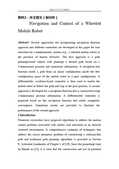
附件2:外文原文(复印件)Navigation and Control of a Wheeled Mobile RobotAbstract:Several approaches for incorporating navigation function approach into different controllers are developed in this paper for task execution by a nonholonomic system (e.g., a wheeled mobile robot) in the presence of known obstacles. The first approach is a path planning-based control with planning a desired path based on a 3-dimensional position and orientation information. A navigation-like function yields a path from an initial configuration inside the free configuration space of the mobile robot to a goal configuration. A differentiable, oscillator-based controller is then used to enable the mobile robot to follow the path and stop at the goal position. A second approach is developed for a navigation function that is constructed using 2-dimensional position information. A differentiable controller is proposed based on this navigation function that yields asymptotic convergence. Simulation results are provided to illustrate the performance of the second approach.1 IntroductionNumerous researchers have proposed algorithms to address the motion control problem associated with robotic task execution in an obstacle cluttered environment. A comprehensive summary of techniques that address the classic geometric problem of constructing a collision-free path and traditional path planning algorithms is provided in Section 9, .Literature Landmarks of Chapter 1 of [19]. Since the pioneering work by Khatib in [13], it is clear that the construction and use of potentialfunctions has continued to be one of the mainstream approaches to robotic task execution among known obstacles. In short, potential functions produce a repulsive potential field around the robot workspace boundary and obstacles and an attractive potential Þeld at the goal configuration. A comprehensive overview of research directed at potential functions is provided in [19]. One of criticisms of the potential function approach is that local minima can occur that can cause the robot to get stuck without reaching the goal position. Several researchers have proposed approaches to address the local minima issue (e.g., see [2],[3], [5], [14], [25]). One approach to address the local minima issue was provided by Koditschek in [16] for holonomic systems (see also [17] and [22]) that is based on a special kind of potential function, coined a navigation function, that has a refined mathematical structure which guarantees a unique minimum exists. By leveraging from previous results directed at classic (holonomic) systems, more recent research has focused on the development of potential function-based approaches for more challenging nonholonomic systems (e.g., wheeled mobile robots (WMRs)). For example, Laumond et al. [18] used a geometric path planner to generate a collision-free path that ignores the nonholonomic constraints of a WMR, and then divided the geometric path into smaller paths that satisfy the nonholonomic constraints, and then applied an optimization routine to reduce the path length. In [10] and [11], Guldner et al. use discontinuous, sliding mode controllers to force the position of a WMR to track the negative gradient of a potential function and to force the orientation to align with the negative gradient. In [1], [15], and [21], continuous potential field-based controllers are developed to also ensure position tracking of the negative gradient of a potential function, and orientation tracking of the negative gradient. More recently, Ge and Cui present a new repulsive potential function approach in [9] to address thecase when the goal is non-reachable with obstacles nearby (GNRON). In [23] and [24], Tanner et al. exploit the navigation function research of [22] along with a dipolar potential field concept to develop a navigation function-based controller for a nonholonomic mobile manipulator. Specifically, the results in [23] and [24] use a discontinuous controller to track the negative gradient of the navigation function, where a nonsmooth dipolar potential field causes the WMR to turn in place at the goal position to align with a desired orientation. In this paper, two different methods are proposed to achieve a navigation objective for a nonholonomic system. In the first approach, a 3-dimensional (3D) navigation-like function-based desired trajectory is generated that is proven to ultimately approach to the goal position and orientation that is a unique minimum over the WMR free configuration space. A continuous control structure is then utilized that enables the WMR to follow the path and stop at the goal position and orientation set point (i.e., the controller solves the unified tracking and regulation problem). The unique aspect of this approach is that the WMR reaches the goal position with a desired orientation and is not required to turn in place as in many of the previous results. As described in [4] and [20], factors such as the radial reduction phenomena, the ability to more effectively penalize the robot for leaving the desired contour, the ability to incorporate invariance to the task execution speed, and the improved ability to achieve task coordination and synchronization provide motivation to encapsulate the desired trajectory in terms of the current position and orientation. For the on-line 2D problem, a continuous controller is designed to navigate the WMR along the negative gradient of a navigation function to the goal position. As in many of the previous results, the orientation for the on-line 2D approach requires additional development (e.g., a separate regulation controller; a dipolar potential field approach [23], [24]; or a virtualobstacle [9]) to align the WMR with a desired orientation. Simulation results are provided to illustrate the performance of the second approach.2 Kinematic ModelThe class of nonholonomic systems considered in this paper can be modeled as a kinematic wheelwhere are defined asIn (1), the matrix is defined as followsand the velocity vector is defined aswith vc(t), ωc(t) ∈R denoting the linear and angular velocity of the system. In (2), xc(t), yc(t), and θ(t) ∈R denote the position and orientation, respectively, xc(t), yc(t) denote the Cartesian components of the linear velocity, and θ(t) ∈ R denotes the angular velocity.3 Control ObjectiveThe control objective in this paper is to navigate a non-holonomic system (e.g., a wheeled mobile robot) along a collision-free path to a constant,goal position and orientation, denoted by , in an obstacle cluttered environment with known obstacles. Specifically, the objective is to control the non-holonomic system along a path from an initial position and orientation to q∗∈D, where D denotes a free configuration space. The free configuration space D is a subset of thewhole configuration space with all configurations removed that involve a collision with an obstacle. To quantify the path planning-based control objective, the difference between the actual Cartesian position and orientation and the desired position and orientation, denotedby, is defined asas followswhere the desired trajectory is designed so that qd(t) → q∗. Motived by the navigation function approach in [16], a navigation-like function is utilized to generate the desired path qd(t). Specifically, the navigation-like function used in this paper is defined as follows Definition 1 Let D be a compact connected analytic manifold with boundary, and let q∗be a goal point in the interior of D. The navigation-like function ϕ(q): D →[0, 1], is a function satisfies the following properties:1. ϕ (q(t)) is first order and second order differentiable (i.e., and´exist on D).2. ϕ (q(t)) obtains its maximum value on the boundary of D.3. ϕ (q(t)) has unique global minimum at q (t) = q∗.4. If with εz, εr ∈ R being known positive constants.5. If ϕ(q(t)) is ultimately bounded by ε, then is ultimately bounded by εr with ε∈ R being some known positive constant.4 Online 3D Path Planner4.1 Trajectory PlanningThe 3D desired trajectory can be generated online as followswhere ϕ(q) ∈ R denotes a navigation-like function defined in Definition1, denotes the gradient vector of ϕ(q), and is anadditional control term to be designed. Assumption The navigation-like function defined in Definition 1 along with the desired trajectory generated by (6) ensures an auxiliary terms N (·) ∈ R3, defined assatisfy the following inequalitywhere the positive function ρ (·) is nondecreasing in and . The inequality given by (8) will be used in the subsequent stability analysis.4.2 Model TransformationTo achieve the control objective, a controller must be designed to track the desired trajectory developed in (6) and stop at the goal position q∗. To this end, the unified tracking and regulation controller presented in [7] can be used. To develop the controller in [7], the open-loop error system defined in (5) must be transformed into a suitable form. Specifically, the position and orientation tracking error signals defined in (5) are related to the auxiliary tracking error variables w(t) ∈R and through the following global invertible transformation [8]After taking the time derivative of (9) and using (1)-(5) and (9), the tracking error dynamics can be expressed in terms of the auxiliary variables defined in (9) as follows [8]where denotes a skew-symmetric matrix defined asand is defined asThe auxiliary control input introduced in (10)is defined in terms of and as follows4.3 Control DevelopmentTo facilitate the control development, an auxiliary error signal, denotedby, is defined as the difference between the subsequentlydesigned dynamic oscillator-like signal and the transformed variable z(t), defined in (9), as followsBased on the open-loop kinematic system given in (10) and the subsequent stability analysis, we design u(t) as follows [7]where k2 ∈ R is a positive, constant control gain. The auxiliary control term introduced in (15) is defined aswhere the auxiliary signal zd(t) is defined by the following differential equation and initial conditionThe auxiliary terms Ω1 (w, f, t) ∈ R and δd(t) ∈ R are defined asandrespectively, k1, α0, α1, ε1 ∈R are positive, constant control gains, and was defined in (12). As described in [8], motivation for the structure of (17) and (19) is based on the fact thatBased on (9), e (t) can be expressed in terms of,and zd (t) as followswhere are defined as followsMotivated by the subsequent stability analysis, the additional control term vr (t) in (6) is designed as followswhere k3, k4 ∈R denotes positive, constant control gains, and the positive functions ρ1 (zd1, z1, qd, e),ρ2 (zd1, z1, qd, e) ∈ R are defined as follows4.4 Closed-loop Error SystemAfter substituting (15) into (10), the dynamics for w(t) can be obtained as followswhere (14) and the properties of J in (11) were utilized. After substituting (16) into (26) for only the second occurrence of ua(t), utilizing (20) and the properties of J in (11), the final expression for the closed-loop error system for w(t) can be obtained as followsTo determine the closed-loop error system for, we take the timederivative of (14) and then substitute (10) and (17) into the resulting expression to obtain the following expressionAfter substituting (15) and (16) into (28), (28) can be rewritten as followsAfter substituting (18) into (29) for only the second occurrence of Ω1 (t) and then canceling common terms, the following expression can be obtainedSince the bracketed term in (30) is equal to ua (t) defined in (16), the final expression for the closed-loop error system for can be obtained asfollowsRemark 1 Based on the fact that δd (t) of (19) exponentially approachesan arbitrarily small constant, the potential singularities in (16), (17), and (18) are always avoided.4.5 Stability AnalysisTheorem 1 Provided qd (0) ∈ D, the desired trajectory generated by (6) along with the additional control term vr (t) designed in (24) ensures thatand.where εr is defined in Definition 1.Proof: Let V (t) ∈ R denote the following functionwhere k ∈R is a positive constant, V1 (t) ∈R denotes the following functionand V2 (qd) : D → R denotes a function as followsAfter taking the time derivative of (33) and then substituting (27) and (31) into the resulting expression and cancelling common terms, the following expression can be obtainedAfter taking the time derivative of (34) and utilizing (6), the following expression can be obtainedwhere N (·) is defined in (7). Based on (8), úV2 (t) can be upper bounded as followsAfter substituting (21) into (37), the following inequality can be obtainedwhere the vector is defined as followsand the positive function ρ1 (zd1, z1, qd, e) andρ2 (zd1, z1, qd, e) are defined in (25). After substituting (24) into (38), V2 (t) can be rewritten as followsBased on (35) and (40), the time derivative of V (t) in (32) can be upper bounded by the following inequalitywhere the positive constant are defined as followsCase 1: If , from the Property 4 in Definition 1, it is clearthatCase 2: If , it is clear from (32), (33), (34), and (41) thatwhere and are positive constants. Based on (42), V (t) can be upper bounded as followsthereforeBased on (32), (34), and (44), it is clear thatIf qd (0) is not on the boundary of D, ϕ(qd (0)) < 1. Then k can be adjusted to ensureBased on (45) and (46), ϕ (qd (t)) < 1, hence qd (t) ∈ D from Definition1. It is clearly from (43) that ϕ (qd) is ultimately bounded by²z. Therefore, if, k4 can be adjusted to ensure, whereε is defined in Definition 1. Hence by the Property 5 in Definition 1,is ultimately bounded by εr.¤Theorem 2 The kinematic control law given in (15)-(19) ensures global uniformly ultimately bounded (GUUB) position and orientation tracking in the sense thatwhere ε1 was given in (19), , and ε3and γ0 are positive constants. Proof: Based on (33) and (35), V1 (t) of (35) can be upper bounded as followsBased on (48), the following inequality can be obtainedBased on (33), (49) can be rewritten as followswhere the vector Ψ1 (t) is de fined in (39). From (33) and (49), it is clear that w (t) ,∈L∞. Based on (19) and (20), we can conclude that zd (t)∈ L∞. From (14) and, zd (t) ∈ L∞, it is clear that z (t) ∈ L∞. Since w(t), z (t) ∈ L∞, based on the inverse transformation from (9), e (t) ∈L∞. Based on qd (t) ∈ L∞ from Theorem 1 and e (t) ∈ L∞, it is clear that q (t) ∈ L∞. From (22)-(25), qd (t), zd (t), z (t), e (t) ∈ L∞, and the properties in Definition 1, we can conclude that vr (t), qd (t) ∈ L∞. Based on (12) and q (t), z (t), qd (t) ∈ L∞, f (θ, z2, qd) ∈ L∞. Then Ω1 (t) ∈ L∞ from(18). Then u (t), ua (t), zd (t) ∈ L∞ from (15)-(17). Based on the fact thatf (θ, z2, qd), z (t), u (t) ∈ L∞, then (10) can be used to conclude w (t), z (t) ∈ L∞. It is clear from z(t) , zd (t) ∈ L∞ that∈ L∞. Then standard signal chasing arguments can be employed to conclude that all of the remaining signals in the control and the system remain bounded during closed-loop operation.Based on (19), (20), (39), and (50), the triangle inequality can be applied to (14) to prove thatUtilizing (50)-(51), the result given in (47) can be obtained from taking the inverse of the transformation given in (9). ¤Remark 2 Although qd (t) is a collision-free path, the stability result in Theorem 2 only ensures practical tracking of the path in the sense that the actual WMR trajectory is only guaranteed to remain in a neighborhood of the desired path. From (5) and (47), the following bound can bedevelopedwhere qd (t) ∈ D based on the proof for Theorem 1. To ensure that q (t) ∈ D, the free configuration space needs to be reduced to incorporate the effects of the second and third terms on the right hand side of (52). To this end, the size of the obstacles could be increased by, where ε3ε1 can be made arbitrarily small by adjusting the control gains. To minimize the effects of ε2, the initial conditions w (0) and z (0) (and hence, could be required to be sufficiently small enough to yield a feasible path to the goal.5 Online 2D NavigationIn the previous approach, the size of the obstacles is required to be increased due to the fact that the navigation-like function is formulated in terms of the desired trajectory. In the following approach, the navigation function proposed in [22] is formulated based on current position feedback, and hence, q (t) can be proven to be a member of D without placing restrictions on the initial conditions.5.1 Trajectory PlanningLet ϕ(xc, yc) ∈R denote a 2D position-based navigation function defined in D that is generated online, where the gradient vector of ϕ(xc, yc) is defined as followsLet θd (xc, yc) ∈R denote a desired orientation that is defined as a function of the negated gradient of the 2D navigation function as followswhere arctan 2 (·) : R2 → R denotes the four quadrant inverse tangent function [26], where θd (t) is confined to the followingregion As stated in [21], by defining, then θd(t) remains continuous alongany approaching direction to the goal position. See Appendix for an expression for θd(t) based on the previous continuous definition for θd(t). Remark 3 As discussed in [22], the construction of the function ϕ(q(t)), coined a navigation function, that satisfies the first three properties in Definition 1 for a general obstacle avoidance problem is nontrivial. Indeed, for a typical obstacle avoidance, it does not seem possible toconstruct ϕ(q(t)) such that only at q (t) = q∗. That is, as discussed in [22], the appearance of interior saddle points (i.e., unstable equilibria) seems to be unavoidable; however, these unstable equilibria do not really cause any difficulty in practice. That is, ϕ(q(t)) can be constructed as shown in [22] such that only a .few. initial conditions will actually get stuck on the unstable equilibria. 5.2 Control Development Based on the open-loop system introduced in (1)-(4) and the subsequent stability analysis, the linear velocity control input vc (t) is designed as followswhere kv ∈R denotes a positive, constant control gain, and was introduced in (5). After substituting (55) into (1), the following closed-loop system can be obtainedThe open-loop orientation tracking error system can be obtained bytaking the time derivative of in (5) as followswhere (1) was utilized. Based on (57), the angular velocity control inputωc (t) is designed as followswhere kω ∈ R denotes a positive, constant control gain, and θd(t) denotes the time derivative of the desired orientation. See Appendix for an explicit expression forθd (t). After substituting (58) into (57), the closed-loop orientation tracking error system is given by the following linear relationshipLinear analysis techniques can be used to solve (59) as followsAfter substituting (60) into (56) the following closed-loop error system can be determined5.3 Stability AnalysisTheorem 3 The control input designed in (55) and (58) along with the navigation function ensure asymptotic navigation in the sense thatProof: Let: D → R denote the following non-negative functionAfter taking the time derivative of (63) and utilizing (1), (53), and (56), the following expression can be obtainedBased on the development provided in Appendix, the gradient of thenavigation function can be expressed as followsAfter substituting (65) into (64), the following expression can be obtainedAfter utilizing a trigonometric identity, (66) can be rewritten as followswhere g(t) ∈ R denotes the following positive functionBased on (53) and the property of the navigation function (Similar to theProperty 1 of Definition 1), it is clear that on D; hence, (55) can be used to conclude that vc (t) ∈ L∞ on D. Development is also provided in the Appendix that proves θd (t) ∈ L∞ on D; hence, (58) can be used to show that ωc (t) ∈ L∞ on D. Based on the fact that vc (t) ∈L∞ on D, (1)-(4) can be used to prove that xc (t), yc (t) ∈ L∞ on D. After taking the time derivative of (53) the following expression can be obtainedSince xc (t), yc (t) ∈L∞ on D, and since each element of the Hessian matrix in (69) is bounded by the property of the navigation function (Similar to the Property 1 ofDefinition 1), it is clear that gú(t) ∈ L∞ on D. Based on (63), (67), (68), and the fact that g(t) ∈ L∞ on D, then Lemma A.6 of [6] can be invoked to prove thatin the region D. Based on the fact that 1 from (60), then (70)can be used to prove that. Therefore the result in (62) can be obtained based on the analysis in Remark 3. ¤Remark 4 The control development in this section is based on a 2D position navigation function. To achieve the objective, a desired orientation θd (t) was defined as a function of the negated gradient of the 2D navigation function. The previous development can be used to provethe result in (62). If a navigation function can be found suchthat, then asymptotic navigation can be achieved by the controller in (55) and (58); otherwise, a standard regulation controller (e.g., see [8] for several candidates) could be implemented to regulate theorientation of the WMR from. Alternatively, a dipolar potential field approach [23], [24] or a virtual obstacle [9] could be utilized to align the gradient field of the navigation function to the goal orientation of the WMR.6 Simulation ResultsTo illustrate the performance of the controller given in (55) and (58), a numerical simulation was performed to navigate the WMR fromto.Since the properties of a navigation function are invariant under a diffeomorphism, a diffeomorphism is developed to map the WMR free configuration space to a model space [17]. Specifically, a positive function was chosen as followswhere κ is positive integer parameter, and the boundary functionand the obstacle function are defined as followsIn (72), and are the centers of the boundary and the obstacle respectively, r0, r1 ∈R are the radii of the boundary and the obstacle respectively. From (71) and (72), it is clear that the model space is a unit circle that excludes a circle described by the obstaclefunction. If more obstacles are present, the corresponding obstacle functions can be easily incorporated into the navigation function [17]. In [17], Koditschek proved that in (71) is the navigationfunction for, provided that κ is big enough. For the simulation, the model space configuration is selected as followswhere the initial and goal configuration were selected asThe control inputs defined in (55) and (58) were utilized to drive the WMR to the goal point along the negated gradient angle. The control gains kv and kω were adjusted to the following values to yield the best performanceOnce the WMR reached the goal position, the regulation controller in [8]was implemented to regulate the WMR from . The actual trajectory of WMR is shown in Figure 1. The outer circle in Figure1 depicts the outer boundary of the obstacle free space and the inner circle represents the boundary around an obstacle. The resulting position and orientation errors for the WMR are depicted in Figure 2, where therotational error shown in Figure 2 is the error between the actual orientation and goal orientation. The control in-put velocities vc(t) and ωc(t) defined in (55) and (58), respectively, are depicted in Figure 3. Note that the angular velocity input was artificially saturated between ±90[deg ·s−1].7 ConclusionsTwo approaches are developed to incorporate navigation function approach into different controllers for task execution by a WMR in the presence of known obstacles. The first approach utilizes a navigation-like function that is based on 3D position and orientation information. The navigation-like function yields a path from an initial configuration inside the free configuration space to a goal configuration. A differentiable, oscillator-based controller is then used to enable the mobile robot to follow the path and stop at the goal position. Using this approach, a WMR was proven to yield uniformly ultimately bounded path following and regulation to the goal point with an arbitrarily defined goal orientation (i.e., the WMR is not required to spin in place at the goal position to achieve a desired orientation). A second approach is developed that uses a navigation function that is constructed using 2D position information. A differentiable controller is proposed based on this navigation function. The advantage of this approach is that it yieldsasymptotic position convergence; however, the WMR cannot stop at an arbitrary orientation without additional development. Simulation results are provided to illustrate the performance of the second approach. AppendixBased on the definition of θd (t) in (54), θd (t) can be expressed in terms of the natural logarithm as follows [26]where . After exploiting the following identities [26]and then utilizing (74) the following expressions can be obtainedAfter utilizing (75) and (76), the following expression can be obtainedBased on the expression in (74), the time derivative of θd (t) can be written as followswhere·After substituting (1), (79), and (80) into (78), the following expression can be obtainedAfter substituting (55) and (77) into (81), the following expression can be obtained¸.By part 1 of Definition 1, each element of the Hessian matrix is bounded;hence, from (82), it is straightforward that。
全向舵轮移动机器人控制算法

全向舵轮移动机器人控制算法
全向舵轮移动机器人的控制算法主要包括以下几个方面:
1.路径规划:根据机器人的目标点和环境信息,规划出一条从起点到终点的
最优或次优路径。
常见的路径规划算法有A*算法、Dijkstra算法、模糊逻辑算法等。
2.速度控制:根据机器人的当前位置、目标位置和环境信息,计算出机器人
的行进速度,使得机器人能够以最短的时间或最优的路径到达目标位置。
常见的速度控制算法有PID控制算法、模糊控制算法等。
3.方向控制:根据机器人的当前朝向和目标朝向,计算出机器人的转向角度,
使得机器人能够以最短的时间或最优的路径到达目标位置。
常见的方向控制算法有比例控制算法、模糊控制算法等。
4.避障控制:根据机器人周围的环境信息,判断是否存在障碍物,并计算出
机器人的转向角度或行进速度,以避免与障碍物发生碰撞。
常见的避障控制算法有超声波传感器避障算法、红外传感器避障算法、激光雷达传感器避障算法等。
总之,全向舵轮移动机器人的控制算法需要考虑多个方面,包括路径规划、速度控制、方向控制和避障控制等。
需要根据实际应用场景和机器人自身特点选择合适的算法,以达到最优的控制效果。
- 1、下载文档前请自行甄别文档内容的完整性,平台不提供额外的编辑、内容补充、找答案等附加服务。
- 2、"仅部分预览"的文档,不可在线预览部分如存在完整性等问题,可反馈申请退款(可完整预览的文档不适用该条件!)。
- 3、如文档侵犯您的权益,请联系客服反馈,我们会尽快为您处理(人工客服工作时间:9:00-18:30)。
全向轮移动机器人的设计和控制
050308225 Alex.Wang
摘要
这篇论文介绍一个全向移动机器人作为教育学习。
由于它的全向轮设计,这种机器人拥有有各个方向移动的能力。
这篇论文主要提供了一些关于常用的和特殊的车轮设计,以及全向轮机械设计方面和电子控制方法:远程控制、自动导航寻迹和自动控制的方法。
1、引言
移动机器人在工业和技术方面应用的重要性正在日益的增加,在无人监控值守、检查作业、运输运送领域已经得到了广泛的应用。
一个更加紧俏的市场是移动娱乐机器人的开发。
作为一个全自动的移动机器人,其中一个主要的应用需求是它的空间移动能力,同时能够避免障碍物并且发现去下一站的路径。
为了能实现这种任务,能够引导机器人移动的功能如定位、导航必须为机器人提供他当前位置信息,这就意味着,它要借助于多个传感器,外部的状态参考和算法。
为实现移动机器人能够在狭窄的区域移动并且避开障碍物,必须具备良好的移动性能并得到正确而巧妙的引导,这些能力主要取决于车轮的设计。
关于这方面的研究正在持续不断的进行,以改善移动机器人系统的自动导航能力。
本篇论文介绍一种全方向的移动机器人作为教育之用。
采用特殊的Mecanum轮设计,使这种机器人拥有全部方向的移动能力。
论文目前提供一些关于传统的和特殊的车轮设计、机械结构设计以及电路和控制方法、远程遥控、线性跟踪(LINE FOLLOW)、自动控制方面的信息。
由于这种机器人的移动能力和它各种控制方法的多样选择性,本章中讨论的机器人可以作为一个非常有趣的教育性平台。
这篇论文是一项在Robotics Laboratory of the Mechanical Engineering Faculty, ”Gh. Asachi” Iasi理工大学研究成果的总结报告。
2、全方向移动能力
“全方向”这个术语是用来描述一个系统在任意的环境结构中立刻向某一方向移动的能力。
机器人型运动装置通常是为在平坦的平面上移动而设计的,运行在仓库地面、路面、LAKE、桌面等。
在这种二维的空间,一个物体有三个自由的维度,能够在各种方向之间转换并且能够以物体的重心为中心进行旋转,但是很多传统的车辆不能独立地控制每个方向的度数。
传统的车轮不能够向平行于轮轴的方向移动,这种所谓的非完整的限制车轮阻止了车辆使用侧向滑动,比如小汽车,向垂直于行驶的方向移动。
虽然它能够在一个二维的空间基本达到每个位置和方向,但需要复杂而巧妙的引导和复杂的路径来完成。
这种情况在人工操作和自动驾驶的车辆上都是存在的。
当一个车辆没有完整性的限制(holonomic constraints),它可以在任何方位驶向每一个方向,这种能力就是被广泛熟知的全向移动能力。
全向移动装置在常规的(non-holonomic)的平台上拥有非常大的优势,伴随像汽车一样的阿克曼(车)转向驾驶盘或者不同的驾驶系统,在狭窄的区域移动。
它们可以在狭窄的小道上横行或斜行、原地转向或者沿着复杂的轨道移动。
这种机器人可以在有固定或者活动的障碍物以及狭窄的小道等复杂环境中轻松的完成任务,这种环境通常可以在工厂车间、办公室、仓库以及医院等地方发现。
灵活的材料处理和运动,加上实时的控制已经成为现代制造业一个基本的部分。
自动引导的移动装置(VGA’S)在灵活的制造系统中用来移动和调节部件而得到了广泛的应用。
全向移动装置发展的未来是更进一步的提高这种结构的有效性,并且增加一个可以测试车辆特殊的机动性的地面行驶平台。
全向移动装置根据移动性能而排列的车轮可以分为两类:常规的车轮设计和特殊的车轮设计。
三、车轮设计
1、传统的车轮设计
传统的用于拥有全向移动能力的机器人的车轮设计可以分为两个类型,脚轮(caster wheels)和方向轮(steering wheels)。
与特殊的车轮配置相比,它们拥有更好的路面适应能力
并且能更好的承受地面的不规则(irregularities)。
但是,由于他们非完整的特性而并不拥有真正的全向性,因为当遇到沿着一个不连续的弯道移动时只有很有限的时间让转向马达驱动车轮以重新适应那个设计好的弯道。
在大多数应用中这个过程通常所需的时间比整车辆的动力学快的多。
因此,可以认为他是可以实现零半径轨迹运行的并且保留了全方位这个术语的称号。
大多数包含传统轮子和近似全方位的移动机构,至少是将两个独立控制和独立驱动的轮子组合在一起的。
活动的小脚轮(Castor wheels)或者是传统的方向轮(steered wheels)可以用来实现这种近似的全方位移动能力。
2、特殊的车轮设计
特殊的车轮是基于活动有效的牵引力在一个方向,而允许被动移动在另外一个方向这样的概念而设计的,因此在拥挤的环境中拥有了更大的灵活性。
这种设计中包含了普通的车轮、Mecanum(Swedish)轮和球形轮这种机械结构。
一般的车轮结构在转向中提供了一种限制性的和非限制性相结合的移动能力。
这种机械装置在车轮的直径外围安装了多个小滚轮,这样的车轮可以正常的转动,同时可以在平行于轮轴中心线的方向自由的滚动。
车轮可以完成这种动作是因为小滚轮和车轮旋转时的中心轴线是相垂直安装的。
当两个或者更多的这种车轮安装在运载平台上,他们这种限制性和非限制性相结合的移动为全向移动能力提供了可能。
Mecanum(Swedish)轮在设计上和普通的轮子非常的相似,除了它周围有很多按角度均分镶嵌镶嵌的小轮,如图1所示。
这种结构把一部分沿轮子旋转方向的力转化成了垂直于轮子旋转方向的力。
这种平台构造由四个车轮组成,就像一辆小汽车那样。
由于每个轮子不同的旋转方向和转速,四个车轮各自受的力所形成的合力是一个矢量,这就为移动装置转向任一方向提供了可能。
另外一个特殊的车轮设计是球形的车轮机械结构。
它使用一个由马达和变速器驱动的活动圆环来通过摩擦力将能量从小滚轮传递到球形轮上,这样球形轮能够立刻的向某一方向旋转。
四、Mecanum Wheel 的结构设计
更为常见的全方位轮的设计是Mecanum 轮,由一个在瑞典AB 公司的工程师Bengt Ilon 于1973年发明。
车轮由一个轮轴携带一些和轮轴圆周呈45度角的能自由移动的小滚轮组成。
小滚轮的轴线和主轮轴线间的夹角理论上可以是任意的值,但是在Swedish 轮中通常是呈45度角。
边缘呈一定角度的小滚轮将一部分沿轮子旋转方向的力转化成了垂直于轮子旋转方向的力。
根据各个轮子的旋转方向和速度,这些力的合力形成了一个新的矢量指向需要的方向,因而能够让移动平台自由地沿着合力矢量方向移动而不需要改变车轮的转向。
图 4-1 Mecanum Wheel
小滚轮的形状正如全方位轮的轮廓在图1中所示。
我们可以通过削割圆柱得到小滚轮的形状,(具有外部直径的车轮),在同一个平面里的角度(小滚轮和轮轴线的角度)γ=45°。
这种模型符合方程:
222102
x y R +-= (1) R 是轮子外部的半径长度。
如果小滚轮的长度Lr 比轮子的外部半径R 小很多,那么小滚轮的形状就和一个以2R 为半径的圆环差不多。
为了使轮子的外形轮廓是圆形的,小滚轮的最小数量应该计算出来(如图4-2)。
图4-2 轮子的设计参数 根据图4-2,如果小滚轮的长度参数Lr 确定了,那么可以得出小滚轮的数量n ,
2n πϕ=
(2)
其中: 2arcsin 2sin r L R ϕγ⎛⎫=
⎪⎝⎭ (3) 如果我们假设小滚轮的数量n 是知道的,同样我们可以得出小滚轮的长度:
sin sin
222sin sin r n L R
R πϕγγ
== (4) 轮子的宽度为: sin
cos 2sin w r n l L R
πγγ
== (5) 本文中已知γ=45°,可得:
sin r L n π
= (6)
2sin w l R n π
= (7)
小滚轮既不具有驱动能力也没有感知能力。
这种设计的关键优势是,尽管单个轮子的转动只由主轮轴驱动,每个轮子可以沿着多种轨迹方向伴随着一些摩擦力实现运动学上的移动,而不是仅仅的向前或者向后运动。
一个Swedish 全方位轮拥有三个方向的自由度,包括轮子的转动、小滚轮的转动和
伴
随着垂直于轮面的轴通过与地面的接触点时转动而产生的滑动(如图4-3)。
在全方位轮中,车轮的速率可以分解为有效活动的方向和被动的方向两个部分。
活动有效部分的方向是和与地面相接触的小滚轮轴线相重合的,而被动部分的方向是和小滚轮的轴线相垂直的。
图4-3 Mecanum Wheel 的自由度
五、电子学控制功能设计
正如我们前面提到的,可以使用一种命令系统让这种机器人实现远程控制,也可以让它沿着轨迹运动或者使用一种超声波传感器自动避让障碍物实现自动导航。
图6-1 控制系统
为了接收图6-1中控制系统提供的信号,或者是探测障碍物并且控制马达运行,基于PIC16F876 微控制器的芯片主板放置于机器人使用(如图6-2)。
图6-2 电子芯片主板。