Overview Real-time logic Counting true instances
real-time的基础知识.doc

理论基础聚合酶链式反应作为一种革命性的方法在生物学研究的历史中占据了重要的地位。
以此为基础发展出包括real-time PCR在内的多项应用技术。
自诞生后real-time PCR技术持续发展,从简单的增扩到整个PCR过程,real-time PCR表现出比PCR更敏感、更明确的定量分析特性和对识别等位基因的能力。
不少人以为real-time就是意味着可以在显示器上看到每个循环增扩曲线的增长。
事实并非如此,早期的软件不能在运行期间提供可视化的增扩曲线。
主要是因为SDS软件采用整个平台最终的数据执行数据分析工作,而不是分析每个单独的反应循环。
对某些设备来说,必须向分析软件提供实时的最终的数据,有些设备则不需要。
前一种设备允许软件实时跟踪每个加样口的增扩曲线,同时显示在电脑屏幕上。
Real-time PCR其实是一种real-time设备。
RNA定量分析依靠逆转录酶制作cDNA (complementary DNA)O常见的逆转录酶有2种,AMV 和MMLVo AMV是一种鸟类myeloblastosis病毒的二聚体蛋白质,MMLV来自于鼠科leukemia 病毒的monomeric蛋白。
2种酶都有RNase把RNA变性为RNA-DNA杂交体的活性,比较而言AMV 有更高的RNase H活性。
RNase H活性和依赖于RNA的DNA聚合酶活性能被mutagenesis区分开来。
更重要的是每个AMV能把较多的分子聚拢在一起,推动增扩反应的进行。
原生的AMV 有高于MMLV的适用温度,42°C对37°C。
修改后的变种可以有更高的温度极限,分别是AMV58 °C, MMLV55C按照以上的描述,大家可能认为改造后的AMV是适宜从RNA制作cDNA的酶。
然而,在实际使用中经改造的MMLV工作的较好。
其中的原因目前仍不明,猜测高温破坏了2种酶的聚合酶活性,但残留的DNA绑定活性对Taq polymerase形成物理障碍。
real-time方法

real-time方法
在软件开发中,real-time方法通常指的是使用实时操作系统(RTOS)或实时编程技术来开发能够满足严格时间限制的应用程序。
实时操作系统可以保证任务能够在特定的时间间隔内得到处理,而
实时编程技术则可以确保程序能够按时完成任务。
这种方法在需要
高度可靠性和稳定性的系统中得到广泛应用,比如飞行控制系统、
医疗设备等。
另外,在金融交易领域,real-time方法也十分重要。
实时交
易系统需要能够在毫秒甚至微秒级的时间内完成交易,以获取最佳
的交易价格和执行速度。
这就需要使用高性能的实时数据处理和交
易执行系统来实现。
总的来说,real-time方法在不同领域都有着重要的应用,它
们都致力于确保任务或计算能够在严格的时间限制内得到处理或完成。
这需要使用特定的技术和工具来实现,以满足不同领域对实时
性的要求。
全球电离层地图TEC数据的插值算法
0254-6124/2021/41(3)-411-06 Chin. J. Space Sci.空间科学学报Q U Renchao, M I A O Hongli, G O U Ruikun, M A O Peng. Interpolation algorithm of global ionospheric m a p product T E C (in Chinese). Chin. J. Space Sci., 2021, 41(3): 411-416. D01:10.11728/cjss2021.03.411全球电离层地图T E C数据的插值算法+曲仁超苗洪利苟瑞锟毛鹏(中国海洋大学信息科学与工程学院青岛266100)条商要由I G S工作组提供的全球电离层地图(G I M)是电离层重要的应用数据.卫星高度计能够提供全球实时的电离层 延迟误差校正.利用G I M数据.以J a s o n-3时空分辨率进行电离层总电子含fi (T E C)的时间维度插值和空间维度插值,其 中空间维度插值采用了K r i g i n g插值和双线性插值两种方法.计对两种插值方法得到的总电子含量,与平滑处理的Jason-3 高度计cycle80双频延迟校正值转化的总电子含量进行对比分析.结果显示:其与K r i g i n g插值的平均偏差为0.94T E C U,均方根误差为2.73T E C U,相关系数为0.91;与双线性插值的平均偏差为1.43T E C U,均方根误差为6.85T E C U,相关系数 为0.61.这说明K r i g i n g插值方法的精度明显高于双线性插值方法.关键词全球电离层地图,高度计,时间插值,K r i g i n g插值.双线性插值中图分类号P353In te rp o la tio n A lg o rith m of G lo b al Io n o sp h e ricM ap P ro d u c t T E CQU Renchao MIAO Hongli GOU Ruikun MAO Peng(College of Information Science and Engineering, Ocean University of China, Qingdao266100)A b s t r a c t G l o b a l Ionospheric M a p (G I M) is a n i m p o r t a n t ionospheric d a t a p r o d u c t p r o v i d e d b y theI G S w o r k i n g group, w h i c h c a n provide global real-time ionospheric delay error correction for satellitealtimeters. In this study, t e m p o r a l a n d spatial interpolation of Total Electron C o n t e n t(T E C) that derived f r o m G I M d a t a p r o d u c t s w a s p e rformed, w i t h the t e m p o r a l a n d spatial resolution of Jaso n-3altimeter. T w o spatial interpolation m e t h o d s, Krig i n g interpolation a n d Bilinear interpolation, w e r eu s e d in this study. T h e T E C o b t a i n e d b y these interpolation m e t h o d s is c o m p a r e d a n d a n a l y z e dw i t h the T E C value that c o nverted f r o m the dual-frequency delay correction of the s m o o t h e d Jason-3 altimeter cycle80 data. Results s h o w that the m e a n bias b e t w e e n Krig i n g interpolation a n d processed dual-frequency delay correction is 0.94 T E C U,the root m e a n sq u a r e error is 2.73 T E C U a n d the correlation coefficient is 0.91. A s a contrast, these statistics b e t w e e n Bilinear interpolation a n dprocessed dual-frequency delay correction are 1.43 T E C U, 6.85 T E C U, a n d 0.61, respectively. T h i sd e m o n s t r a t e s that the a c c u r a c y of the Kriging interpolation is significantly higher t h a n that of the国家自然科学重点基金项目(62031005)和山东省自然科学基金项目(Z R2020M D097)共同资助2020-03-16收到原稿,2020-12-04收到修定稿E-mail:*************.cn412Chin. J. Space Sci.空间科学学报 2〇21,41(3)Bilinear interpolation.Key words G l o b a l Iono s p h e r e M a p (G I M), T i m e interpolation, Altimeter, Krig i n g interpolation, Bilinear interpolation〇引言全球电离层图(G l o b a l I o n o s p h e r e M a p,G I M)是电离层研究及应用的重要数据来源1998年 电离层分析中心成立了国际G N S S服务组织(I n t e rn a t i o n a l G N S S S e r v i c e,I G S).I G S 将地球电离层看 成一个距地面450k m高的薄球壳,其发布的G I M将全球按经纬方向5° x 2.5°间隔网格化,覆盖范围 为 180°E—180°W,87.5°S_87.5°N,网格点为 71x73, 基于几百个全球卫星导航系统的地面观测站与G P S的双频电子含量观测数据,利用球谐函数及算法得出 每个网格点的总电子含量(T o t a l E l e c t r o n C o n t e n t, T E C),同时以每2h时间分辨率,获得全天13幅 数据.因此,G I M也称为网格模型数据[2-4L随着 全球基准站数量日益增多,G I M精度和可靠性越来 越高,已从1998年的3〜4.5 T E C U提高到2015年 的2〜3.5T E C U.G I M与测高卫星电离层T E C系统 偏差较小,例如相对于J a s o n-2卫星高度计,其系统 偏差约为2.8T E C U15].电离层对微波信号的延迟是卫星髙度计测高的 主要误差来源之一 如J a s o n-3高度计K u波段,电离层引起的测高误差通常为0.2〜40c m.在太阳风 暴活动高发期,电子含量的剧烈变化引起的误差将更 大,对于厘米级雷达高度计测高精度不能接受,必须 给予误差校正.对于双频体制的卫星高度计,利用双 频法可以实时获得信号传播路径的T E C并对电离层 延迟进行较高精度的校正.但对于单频体制的高度 计(例如搭载在天宫二号上的三维成像微波高度计),要进行电离层延迟校正,只能采用模型法,而G I M网格模型数据则是选择之一.在高度计上应用G I M数 据,必须经过进一步的时空插值处理.这是因为高度 计的观测时空分辨率比G I M高得多,需要在时间和 空间两个维度将G I M数据插值到卫星高度计的观测 数据上.常用的空间插值方法有K r i g i n g插值和双线 性插值等.双线性插值由于没有考虑区域的空间相关 性,插值精度不高;而K r i g i n g插值充分考虑了空间 相关性和变异性,具有较高的插值精度.K r i g i n g插值 方法被广泛应用于气象学数据的插值、G P S高程的拟合、土壤成分的变化等领域[8_12】.X i o n g等基于250个G N S S台站的观测数据,采用K r i g i n g插值 方法获得了中国区域的电离层空间结构,并与JPL (J e t P r o p u l s i o n L a b o r a t o r y)提供的 T E C 图作比较. M a o等M利用K r i g i n g方法构建了中讳度区域电 离层T E C图.T a n g等_利用泛K r i g i n g方法构建 了湖南地区电离层T E C地图.本文使用K r i g i n g插值和双线性插值两种方法,将G I M插值到J a s o n-3的c y d e80观测数据的相应 时空位置,并与经平滑和逆运算处理的J a s o n-3双频 电离层T E C数据进行对比,估算两种插值方法的精 度,为单频卫星高度计提供有效的电离层校正方法.1数据处理选取J a s o n-3的c y c l e80的全球数据,并剔除了 这些数据中陆地和内陆湖泊的观测数据,只保留海洋 观测数据,时间范围为2018年4月10日至4月20 日.提取数据中的时间、经度、纬度、电离层双频延迟 校正值,并对电离层双频延迟校正值进行平滑处理,再从I G S官网下载相同时间段的G I M电离层总电 子含量数据,利用△"ion =f2 N t e C,(1)f2逆运算得到对应的总电子含量i V T E C值,从而与 G I M的T E C值比对.式⑴中的频率选取Jason- 3的K u波段,其值为13.58 G H z;A/i ion为电离层路 径延迟值.电离层一般指距离地面50〜1000 k m高度 范围,1000 k m以上电子含量较少.I G S的G I M观 测数据为22000k m高度以下的总电子含量.J a s o n-3卫星轨道高度为1336 k m,基本涵盖了电离层高度. 因此,可以将G I M数据与Jason-3观测的电离层数 据进行比对.本文对比两种插值方法分别获得的T E C值与 时空匹配的J a s o n-3电离层双频延迟值对应的T E C值的平均偏差、均方根误差R M S E和相关系数7■,分 析两种插值方法的优劣.曲仁超等:全球电离层地图T E C 数据的插值算法413180°W180°W180°E图1时间维度T E C 插值Fig. 1 T E C interpolation in time dimension2插值方法在高度计上应用GIM数据.要经过时空插值处理.首先进行时间维度插值,得到任一时刻的G I M,然后在所需时刻的G I M上根据经纬度再进行空间维度插值_2.1时间维度TE C插值对于时间维度的T E C 插值,采用距离加权法. 对任一时刻、任一位置的待插点a :(t ,A ,/3),从相邻时 间点T ,与乃+1对应的两幅G I M网格数据中,选取与该待插点最接近的10个对应网格点数据进行插值,得到所对应时刻的局域GI M插值[气即Z (t) =T j+i —t r !+i-t2Z(Ti) +t ~Tz Ti+i —Z (T l +1).(2)其中,Z ⑴表示任意时刻f 的T E C值.图1所示为其插值.2.2空间维度T E C 插值根据以上得到的时间维度局域GI M插值.采用双线性和K r i g i n g 两种空间捕值方法获取该待插点妁的T E C值.2.2.1双线性插值双线性插值方法如图2所示.其中:待插值点 为:r (A ,/3),其电子总含量为Z (a :);临近的四个点 的经讳度分别为ar 2(A2,j 8i ),》3(乂,卢2),工4(A 2,/32),对应的电子含量分别为以心),Z (:r 2),Z (x 3),Z (x4).首先在经度方向上进行插值,得到;r 5(A ,f t ) 和邱(A ,汍)的总电子含量,Z (x5) =^x[Z {xA ) -Z (x3)] +Z (x3),(3)^2 —M 图2双线性插值Fig. 2 Bilinear interpolationZ(x6) = ^ \Z{x2) - Z{x{)\ + Z(xi ).⑷然后在纬度方向进行插值,由:r d A J O 和:r6(A ,灸) 得到:r(A ,/3)点的总电子含量为Z{x) = ^[Z (x 6) - Z(x5)} + Z{x5). (5)2.2.2 Kriging 插值K r i g i n g插值如图 3 所示•设 ,怎n为G I M的一系列网格点,对应的总电子含量分别为Z(a :i ),Z (a :2),…,之(〜)•根据K r i g i n g 插值方法,待求I 处的电子含量Z 〇r )为相邻区域n 个网格 点的电子含量加权和即nZ(x) = y^(pjZ(xi).(6)i=i其中,也为加权系数,这里选取n 为9个网格点.根据K r i g i n g 插值原则,在保证无偏且估计方差最小的前提下.引入拉格朗日因子/X ,构建拉格朗日z ,a /1 E C UZja/lbCU函数,并求偏导得到关于如下也的联立方程组:71^ <t )a {xi ,xj ) + n = -y (x ,X i),i=l (7)n、E 也二 i .i=l其中,7(a ;i ,a :j )为格网点而与A 间的变异函数值.即l{xi,Xj) = ^E[Z(xi) - Z(xj)]2. (8)Kriging 变异函数种类很多,常见的有线性模型、指数模型、球形模型、高斯模型.选取其中一种模型 作为变异函数,同时联立式(7) (8)得到加权系数也, 再带入式(6)中,得到之⑷.本文选取J a s 〇n -3的c y -c l e 80的双频延迟校正值转化的TE C数据与四种模型插值数据进行对比,结果列于表1.从表1可以看 出:除了高斯模型插值效果较差,其余三种模型均有 较好的插值精度;线性模型公式简单且运算速度比指414图3 K r i g i n g 插值Fig. 3 Kriging interpolation数模型和球形模型快.因此,本文选取线性模型作为 变异函数.3结果分析K r i g i n g插值结果记为Z kr,双线性插值结果记为Zbi.将两个插值结果分别与相同时刻经过平滑处理J a s o n-3的c yd e80双频延迟校正值转化的TE C值进行对比分析.3.1相关度两个插值结果Zk r ,Z b i与Zj a 的散点拟合结果如图4所示.从图4可以看出,K r i g i n g插值与双频延迟校正值转化的T E C值的相关度明显高于双线性插值.前者的相关系数为0.91,均方根差值为2.73TE C U;后者的相关系数为0.61,均方根差值 为 6.85TE C U.3.2 T E C 数值分布插值结果Zk r ,Z b i与Z j a的数值分布如图5(a )(c )所示,局部放大结果如图5(b )⑷所示.图5(a )为4与知的全球T E C数值分布对比,其中横轴Chin . J . Space Sci .空间科学学报 2021,41(3)表1四种K r i g i n g 插值模型统计值T a b le 1C o m p a ris o n o f s ta tis tic a l v a lu e s o ffo u r K rig in g in te rp o la tio n m o d e ls 模型相关系数均方根误差/T E C U线性0.91 2.73指数0.90 2.75球形0.90 2.80高斯0.766.1260no 3i/N zn u a l 'N图4 Z kr, Z b i 与Z ja散点拟合结果Fig. 4 Fitting results of Zkr, Zbi a n dZja scatter-40 -30 -20 10 0 10ATEC/TECU 20 3040 30 -20 -10 0 10 20 30 40ATEC/TECUu 0 20000 40000 60000 80000 10000050000 52000 54000 56000 58000 60000NumberNumber图5 Z kr, Z b i 与Z j a 数值分布.(b) (d )为(a) (c )的局部放大结果Fig. 5 ^kr, Zbi a n d Z\a numerical distribution, (b) (d) are the local amplification results of (a) (c)20000 40000 60000 80000 10000050000 52000 5400056000 58000 60000-------Zja------- Zbi数据序列是对整个c y c l e 80 (10天)数据点进行抽样 处理得到11万多个数据点.为显示插值效果,从中截 取了部分数据进行放大如图5(b )所示,可以看出两 者分布基本吻合,这也反映出两者有较高的相关度. 图5(c )为Z b i与T E C数值分布对比,同样截取相同数据序列进行放大,如图5(d )所示,可以看出两 者一致程度较差.3.3差值概率密度分布I与A 的差值的概率分布如图6(a )所示,Z bi---Zja7060曲仁超等:全球电离层地图T E C 数据的插值算法与Z j a的差值概率分布如图6(b )所示.从图6可以 明显看出:K r i g i n g 插值结果与双频延迟校正值转化 的TE C值更接近,其平均偏差为0.94TE C U;而双线性插值结果与Z j a 平均偏差为1.43TE C U.4结论将I G S发布的GI M数据应用于卫星高度计J a s o n -3 的电离层延迟估计.在 经过时 间维度 T E C插---Zkr(b)41512I 00806()4022o8心 4 2丨丨 00<(>00.0.0.0.0.0.>»11 s U 1>P >>1 l l l q c s q O Ja .wo lbbd o^^J o/ 65 43 21n o 31/33i0331/331图6 Z kr ,Z b i 与Z ja差值概率密度分布Fig. 6 Zkr, ^bi a n d Zja distribution ofdifference probability density416Chin. J. Space Sci.空间科学学报 2021,41(3)值基础上,在空间维度采用K r i g i n g插值和双线性 插值两种方法获得T E C值.分别与经平滑处理后J a s o n-3的c y c l e80双频延迟校正值转化T E C值 作比较.结果表明:K r i g i n g插值结果与双频延迟校 正值转化的T E C值的相关系数为0.91,均方根差 值为2.73T E C U,平均偏差为0.94T E C U;双线性 插值结果与双频延迟校正值转化的T E C值的相关 系数为0.61,均方根差值为6.85T E C U,平均偏差 为 1.43T E C U.由此可以看出,K r i g i n g插值方法明 显优于双线性插值方法.参考文献[1]F E L T E N S J,S C H A E R S.IGS products for the ionosphere [C]//Proceedings of the IGS Analysis Center Workshop. Darmstadt: E S A/E S O C, 1998:225-232[2]C H E N Shangdeng, Y U E Dongjie, LI Ya, et al. Establishment of a regional ionosphere model based on spherical harmonics [J].Mapp.,2015,11:28-32 (陈尚登,岳东杰,李亚,等.基于球谐函数区域电离层模型建立[J].测绘 工程,2015, 11:28-32)[3]R O V I R A-G A R C I A A, J U A N J M, S A N Z J,et al.Accuracy of ionospheric models used in G N S S and SBAS: methodology and analysis [J].J. Geod., 2016, 90(3): 229- 240[4]Z H A N G Qian, W A N G Jian. V T E C reconstruction of theionospheric grid with kriging interpolation [J].10P Conf.Ser.: Earth Environ. Sci., 2019, 237(6): 062001[5]LI Zishen, W A N G Ningbo, LI Min, et al. Evaluation andanalysis of the global ionospheric T E C grid accuracy of the international G N S S service organization [J].J. Geo-p/i y s., 2〇l7, 6〇(10):3718-3729 (李子申,王宁波,李敏,等•国际G N S S服务组织全球电离层T E C格网精度评估与分析[J].地球物理学报,2017, 60(10): 3718-3729)[6]Z H A N G Youguang, JIA Yongjun, F A N Chenqing, et al.H Y-2A satellite radar altimeter error correction algorithmand verification [J].五np. Sci.,2013,15(7): 53-61 (张有广,贾永君,范陈清,等.海洋二号卫星雷达高度计测高误差校正算 法及验证[J]•中国工程科学,2013, 15(7): 53-61)[7]Z H A N G Ting, Z H A N G J i e, C UI Tingwei, et al. Analysisof the ionosphere correct model for the satellite altimeter [J].Remote Sens. Technol. Appli.} 2012, 27(4): 511- 516 (张婷,张杰,崔廷伟,等.卫星高度计电离层校正模型比较 分析[J].遥感技术与应用,2012, 2012, 27(4): 511-516)[8]JIN Fengqiu, H U A N G Zhigang, S H A O Bo. Grid ionospheric delay estimation method based on spatial variabi- l i t y[J]. TleZem. ^reZeconiraZ,2010,31(4): 6-10 (金凤秋,黄 智刚,邵搏.基于空间变异特性的格网电离层延迟估计方法[J].遥测遥控,2010, 31(4):6-10)[9]C U I Shuzhen, Z H O U Jinguo. Accuracy analysis of IGSionospheric m a p by kriging interpolation [J].Global Posit.•S y W.,2016, 41(4): 43 (崔书珍,周金国.克里金插值法内 插I G S电离层图精度分析[J].全球定位系统,2016, 41⑷:43) [10]W A N G Jianli, H A N Xiaodong, W A N G Jiasheng, et alStudy on the spatial interpolation method of ionosphere modeling in regional grids [J].Global Posit.亡.,2015, 40(1): 65-68 (王建立,韩晓冬,王家胜,等.区域格网电离层建 模空间插值方法研究[J].全球定位系统,2015, 40(1): 65-68) [11]X I A Lingjun, G O N G Zhiyu, LI Baizhen. Spatio and temporal distribution of atmospheric C H4 in central China based on G O S A T satellite remote sensing [J].Meteorol.Disaster /?es.,2018, 42(1): 1-8 (夏玲君,巩志宇,李柏贞.基于G O S A T卫星遥感的我国中部地区大气C H4时空 分布[J]•气象与减灾研究,2018, 42(1): 1-8)[12]LI M, Y U A N Y, W A N G N, et al.Statistical comparison of various interpolation algorithms for reconstructing regional grid ionospheric maps over China [J].J. Atmos.Sol.: Terr. Phys, 2018, 172:129-137[13]X I O N G B, W A N W, Y U Y, et al. C O S P A R, 2016. Investigation of ionospheric T E C over China based on G N S Sdata[J]. Adv. Space Res., 2016, 58(6): 867-877[14]M A O Tian, W A N Weixing, S U N Lingfeng. Central andnorthern China T E C m a p using the Kriging method [J J.CTiin. X Space Sci” 2007, 27(4): 279-285 (毛田,万卫星,孙 凌峰.用Kriging方法构建中纬度区域电离层T E C图[J].空间科学学报,2007, 2007, 27(4): 279-285)[15]T A N G Tian, Z H O U Suya, D U Min. Construction of H unan regional ionospheric T E C m a p using Pan-Kriging m ethod [J].Jiangsu Sci. Technol. Inform., 2017, 12:61-62[16]Y U A N Jiangang, LIU Dapeng. Effects of extraction ofG P S ionospheric T E C data using ionex f i l e interpolation [J].Site Invest.Sci. Tec/moZ.,2018, 1:9-12 (袁建 刚,刘大鹏.利用ionex文件插值提取G P S电离层T E C数据 效果研究[J]•勘察科学技术,2018, 1:9-12)[17]H U A N G Changjun, C H E N Yuanhong, Z H O U Lv. Effectsof different spatial interpolation on InSAR atmospheric delay correction [J].Beijing Surv. Mapp.,2018, 6:629- 632 (黄长军,陈元洪,周吕.不同空间插值对I n S A R大气延迟 改正影响研究[J].北京测绘,2018, 6:629-632)[18]Y A N G Mingyuan, LIU Haiyan, JI Xiaolin, et al.Spatio-temporal Kriging optimization for sparsely dispersed data sets [J]. J. Geoin/onn.,2018,20(4): 505-514 (杨明远,刘海 砚,季晓林,等.面向稀疏散布数据集的时空Kriging优化问.地球信息科学学报,2〇18. 2〇(4):5〇5-514)[19]C H E N G L, M A H, Y U D, et al. Extended analysis of realtime f〇F2 mapping in mideastern china based on shortwave signals [J].Radio Sci., 2017, 52(11-12): 1314-1324 [20]W A N G Jianping, LIU Ruiyuan, D E N G Zhongxin. Autocorrelation analysis for interpolation evaluation of iono- spheric T E C[J]. «/. Space 5ci,2019, 39(6): 738-745 (王建 平,刘瑞源,邓忠新.自相关分析法用于电离层T E C的内插评 估[J].空间科学学报,2019, 39(6):73士745)。
计算机专业英语

Unit 1 Computer OverviewText AFoundation of ComputersComputer is electronic equipment which can make arithmetic and logical calculation, process information rapidly and automatically.It was in 1946 that the first computer of the world was invented in America, it is named ENIAC. Though it was very huge and without high performance, it made basis for the development of computers.Since the first computer was born, the development of computer science technique has been quite surprising. Take the speed of calculation for instance, ENIAC could only make calculations 5,000 times per second; but today, the fastest computer can do 100,000,000,000 times.Computers can process various tasks in a variety of areas, such as industry, agriculture, finance, transportation, culture and education, national, defense and family use. In summary, applications of computers may be classified as follows. Science CalculationThe purpose of inventing and developing computer is to make arithmetic calculation rapidly and accurately. Computers can be used for all kinds of science calculation, which have become one of the most important fields of computer application, for example, calculations in the process of launching satellites and missiles, etc.Data ProcessingWith the development of science and technology, more and more information including numerical data and non- numerical data comes out. At present, data processing is the widest field of computer application. Production management, data counting, office automation, traffic dispatching, information retrieval all belong to this field. Especially in recent years, with the development of the database and computer network technique, computer users in different districts and countries can share many valuable information resources through the network.Real-Time ControlReal-time control is the control of procedure in the process of practical productions where computers are applied. Real-time means that the time of computer’s calculating and controlling may match the time of controlled object’s practical running or working.Adjuvant DesignWith its strong ability in calculating and mapping, we can use the computer to improve the quality and efficiency when doing engineering designs in the matter of architecture, machinery and electron. At present, as CAM, CAD and CAI being used very widely, complete automation from design to production has been achieved in many fields.Artificial IntelligenceComputers can simulate people’s feelings and thoughts, replacing part labors ofhuman beings.Text BThe History of ComputersWhile computers are now an important part of the lives of human beings, there was a time when computers did not exist. Knowing the history of computers and how much progress has been made can help you understand just how complicated and innovative the creation of computers really is.Unlike most devices, the computer is one of the few inventions that do not have one specific inventor. Throughout the development of the computer, many people have added their creations to the list required to make a computer work. Some of the inventions extend the types of computers, while others help computers to be further developed.oJ. The BeginningPerhaps the most significant date in the history of computers is the year 1936. It was in this year that the first" computer" was developed. It was created by Konrad Zuse and dubbed the Z1 Computer. This computer stands as the first as it was the first system to be fully programmable. There were devices prior to this, but none had the computing power that sets it apart from other electronics.It wasn't until 1942 that any business saw profit and opportunity in computers. This first company was called ABC computers, owned and operated by John Atanasoff and Clifford Berry. Two years later, the Harvard Mark I computer was developed, furthering the science of computing.Over the course of the next few years, inventors all over the world began to search more into the study of computers, and how to improve upon them. Those next ten years say the introduction of the transistor, which would become a vital part of the inner workings of the computer, the ENIAC I computer, as well as many other types of systems. The ENIAC I is perhaps one of the most interesting, as it required 20 000 vacuum tubes to operate. It was a massive machine, and started the revolution to build smaller and faster computers.The age of computers was forever altered by the introduction of International Business Machines, or IBM, into the computing industry in 1953. This company, over the course of computer history, has been a major player in the development of new systems and servers for public and private use. This introduction brought about the first real signs of competition within computing history, which helped to spur faster and better development of computers. Their first contribution was the IBM 701 EDPMComputer ..J. A Programming Language EvolvesA year later, the first successful high level programming language - FORTRAN was created. This was a programming language not written in "assembly" or binary, which are considered as very low level languages. FORTRAN was written so that more people could begin to program computers easily.The year 1955, the Bank of America, coupled with Stanford Research Institute and General Electric, saw the creation of the first computers for use in banks. The MICR, or Magnetic Ink Character Recognition, coupled with the actual computer, the ERMA, was a breakthrough for the banking industry. It wasn't until 1959 that the pair of systems was put into use in actual banks.In 1958, one of the most important breakthroughs in computer history occurred, the creation of the integrated circuit. This device, also known as the chip, is one of the base requirements for modern computer systems. On every motherboard and card within a computer system, are many chips that contain information on what the boards and cards do. Without these chips, the systems as we know them today cannot function ..J. Gaming, Mice & the InternetFor many computer users now, games are a vital part of the computing experience. 1962 saw the creation of the first computer game, which was created by Steve Russel and MIT, which was dubbed Spacewar.The mouse, one of the most basic components of modern computers, was created in 1964 by Douglass Engelbart. It obtained its name from the "tail" leading out of the device.One of the most important aspects of computers today was invented in 1969. ARPA net was the original Internet, which provided the foundation for the Internet that we know today. This development would result in the evolution of knowledge and business across the entire planet.It wasn't until 1970 that Intel entered the scene with the first dynamic RAM chip, which resulted in an explosion of computer science innovation.On the heels of the RAM chip was the first microprocessor, which was also designed by Intel. These two components, in addition to the chip developed in 1958, would number among the core components of modern computers.A year later, the floppy disk was created, gaining its name from the flexibility of the storage unit. This was the first step in allowing most people to transfer bits of data between unconnected computers.The first networking card was created in 1973, allowing data transfer between connected computers. This is similar to the Internet, but allows for the computers to connect without use of the Internet.-J. Household PC's EmergingThe next three years were very important for computers. This is the timewhen companies began to develop systems for the average consumers. The Scelbi, Mark-8 Altair, IBM 5100, Apple I and II, TRS-80, and the Commodore Pet computers were the forerunners in this area. While expensive, these machines started the trend for computers within common households.One of the most major breakthroughs in computer software occurred in 1978 with the release of the VisiCalc Spreadsheet program. All development costs were paid for within a two-week period of time, which makes this one of the most successful programs in computer history.1979 was perhaps one of the most important years for the home computer users. This is the year that WordStar, the first word processing program, was released to the public for sale. This drastically altered the usefulness of computers for the everyday users.The IBM home computer quickly helped revolutionize the consumer market in 1981, as it was affordable for home owners and standard consumers. 1981 also saw the megagiant Microsoft enter the scene with the MS-DOS operating system. This operating system utterly changed computing forever, as it was easy enough for everyone to learn.-J. The Competition Begins: Apple vs MicrosoftComputers saw yet another vital change during the year of 1983. The Apple Lisa computer was the first with a graphical user interface, or a GUI. Most modern programs contain a GUI, which allows them to be easy to use and pleasing for the eyes. This marked the beginning of the out-dating of most text-based only programs.Beyond this point in computer history, many changes and alterations have occurred, from the Apple-Microsoft wars, to the developing of microcomputers and a variety of computer breakthroughs that have become an accepted part of our daily lives. Without the initial first steps of computer history, none of those would have been possible.Unit 2Text AMicroprocessor Progression: IntelThe following table (Table2-1) helps you to understand the differences between the different processors that Intel has introduced over the years.Table 2-1Information about this table:·The date is the year that the processor was first introduced. Many processors are re-introduced at higher clock speeds for many years after the original release date. ·Transistors is the number of transistors on the chip. You can see the number of transistors on a single chip has risen steadily over the years.·Microns is the width, in microns, of the smallest wire on the chip. For comparison, a human hair is 100 microns thick. As the feature size on the chip goes down, the number of transistors rises.·Clock speed is the maximum rate that the chip can be clocked at, Clock speed will make more sense in the next section.·Date Width is the width of the AUL. An 8-bit AUL can add/subtract/multiply etc. Two 8-bit numbers, while a 32-bit AUL can manipulate 32-bit numbers. An 8-bit AUL world have to execute four instructions to add two 32-bit numbers, while a 32-bit AUL can do it in one instruction. In many cases, the external data bus is the same width as the AUL, but not always. The 8 088 had a 16-bit AUL and 8-bit bus, while the modern Pentiums fetch data 64 bits at a time for their 32-bit AULs. ·MIPS stands for “Millions of Instructions Per Second” and is a rough measure of the performance of a CPU. Modern CPUs can do so many different things the MIPS ratings lose a lot of their meaning, but you can get a general sense of the relative power of the CPUs from this column.From table 2-1 you can see that, in general, there is a relationship between clock speed and MIPS. The maximum clock speed is a function of the manufacturing process and delays within the chip. There is also a relationship between the number of transistors and MIPS. For example, the 8 088 clocked at 5 MHz but only executed at 0.33 MIPS (about one instruction per 15 clock cycles). Modern processors can often execute at a rate of two instructions per clock cycle. The improvement is directly related to the number of transistors on the chip and will make more sense in the next section.Text BMemoryThe memory is that part of a computer in which programs and data are stored. The term "memory" is usually used to refer to the internal storage locations of computer. It is also called real storage or primary storage, and is measured as quantities of K. Each K is equal to 1,024 bytes, and each byte is equal to 8 bits.The principal function of the main memory is to act as an intermediary between the CPU and the rest of the computer system components. It functions as a sort of desktop on which you place the things needed when you begin to work. The CPU can only utilize those software instructions and data that are stored in main memory.As you know, the main memory is a random access memory, or RAM. The name derives from the fact that data can be stored and retrieved at random from anywhere -in the electronic main memory chips in approximately the same amount of time, no matter where the data is.The main memory is in an electronic, or volatile state. When the computer is off,the main memory is empty; when it is on, the main memory is capable of receiving and holding a copy of the software instructions and data necessary for processing. Since main memory is a volatile form of storage that depends on electric power and the power can go off during processing, users often save their work frequently onto nonvolatile secondary storage devices such as diskettes or hard disks. In general, the main memory is used for the following purposes:∙Storage of a copy of the main software program that controls the general operation of the computer. This copy is loaded into the main memory when the computer is turned on (you will find out how later) , and it stays there as long as the computer is on.•Temporary storage of a copy of application program instructions (the specific software you are using in your business) to be retrieved by the CPU forinterpretation and execution.∙Temporary storage of data that was input from the keyboard or other input device until instructions call for the data to be transferred into the CPU for processing . ∙Temporary storage of data that has been produced as a result of processing until instructions call for the data to be used again in subsequent processing or to be transferred to an output device such as the screen, a printer, or a disk storage device.Several kinds of semiconductor memory chips are used in primary storage. Each serves a different purpose ..J. Random-Access-MemoryRandom-Access-Memory (RAM) is used for short-term storage of data or program instructions. The contents of RAM can be read and changed when required. RAM is volatile, which means that if the computer' s electricity supply is disrupted or the computer is turned off, its contents will be lost. Thus, RAM can be used only as a temporary storage ..J. Read-Only MemoryBecause of the advantages in small semiconductor memories, there is a trend in recent years to build some software functions directly into computer chips. Like RAM, these' electronic chips are mounted on boards inside the system unit. Once placed on these chips, programs can be accessed very rapidly. On many microcomputers for example, the operating system is built onto a chip rather than being stored on a floppy disk. This kind of "software in hardware" is called firmware. Several kinds of firmware are available.Read-only Memory (ROM) is by far the most common form of firmware. A ROM module contains a program supplied by the manufacture. The program can be read from the module, but it is impossible for a user to destroy the contents of the module by accidentally writing over them (hence "read-only" ) ..J. Programmable ROM ( PROM)Like ROM, the Programmable ROM (PROM) is nonvolatile and may be written into only once. For the PROM, the written process is performed electrically by a supplier or customer later than the original chip fabrication. Special equipment is required for the writing or "programming" process. PROM can provide flexibility and convenience ..J. Erasable Programmable Read-Only Memory (EPROM)EPROM can be read and written electrically, as with PROM. However, before the writing operation, all the storage cells of the chip must be erased to the same initial state by exposure to ultraviolet radiation. This erasure process can be performed repeatedly; each erasure can take as much as 20 minutes to perform. Thus, the EPROM can be rewritten multiple times, and like the ROM and PROM, holds its data indefinitely. For comparable amounts of storage, the EPROM is more expensive than PROM, but it has the advantage of multiple-update capability..J. Electrically Erasable Programmable Read-Only Memory (EEPROM) EEPROM can be written at any time without erasing prior contents, only the byte or bytes addressed are updated. The writing operation takes considerably longer than the reading operation, about several hundred microseconds per byte. The EEPROM combines the advantage of nonvolatile with the flexibility of being updateable in place, using ordinary bus control, address, and data lines. EEPROM is more expensive than EPROM and is also less dense, supporting fewer bits per chip ..J. Flash MemoryThe newest form of semiconductor memory is the flash memory (so named because of the speed with which it can be reprogrammed). First introduced in the mid-1980s, flash memory is an intermediate between EPROM and EEPROM in both its cost and functionality. Like EEPROM, flash memory uses an electrical erasing technology. An entire flash memory can be erased in one or a few seconds, which is much faster than EPROM. In addition, it is possible to erase just blocks of memory rather than an entire chip. However, flash memory does not provide byte-level erasure. Like EPROM, flash memory uses only one transistor per bit, and so achieves the same density (compared with EEPROM) with EPROM ..J. Cache MemorySome computers are designed with cache memory to increase the speed of transfer of instructions and data from secondary storage to the processor. Like RAM, cache memory is essentially a high-speed temporary storage, area for program instructions and data. However, cache memory is about 10 times faster than RAM. Because its storage capacity is smaller than RAM's capacity, cache memory holds only those instructions and data that the processor needs immediately.<I Decide whether each of the following statements is true or false.1.Main memory is in an electronic or volatile state. When the computer isoff, main memoryis empty.2.RAM is used for short-term storage of data or program instructions.3.Flash memory can provide byte-level erasure.4.Flash memory was first introduced in the mid-1970s.5.PROM is more expensive than EPROM, but it has the advantage of themultiple-update capability .<I Translate the following sentences into Chinese.1.The memory is that part of a computer in which programs and data arestored.2.When the computer is off, the main memory is empty; when it is on, the mainmemory is capable of receiving and holding a copy of the software instructions and data necessary forprocessmg.3.RAM is volatile, which means that if the computer' s electricity supply isdisrupted or the computer is turned off, its contents will be lost.4.For comparable amounts of storage, the EPROM is more expensive thanPROM, but it has the advantage of multiple-update capability.5.Some computers are designed with cache memory to increase the speed oftransfer of instructions and data from secondary storage to the processor.Unit 3 Computer SoftwareText AMicrosoft Visual StudioMicrosoft Visual Studio is the Integrated Development Environment (IDE) from Microsoft. It can be used to develop console and Graphical User Interface applications along with Windows Forms applications, websites, web applications and web services in both native code as well as managed code for all platforms supported by Microsoft Windows, Microsoft Mobile, .NET Framework, .NET Compact Framework and Microsoft Silver Light.Visual Studio includes a code editor supporting IntelliSense as well as code refactoring. The integrated debugger works both as a source-level debugger and amachine-level debugger. Other built-in tools include a forms designer for building GUI applications, web designer, class designer, and database schema designer. It allows plug-ins to be added that enhance the functionality at almost every level-including adding support for source control systems (like Subversion and Visual SourceSafe) and new toolsets like editors and visual designers for domain-specific languages or toolsets for other aspects of the software development lifecycle (like the Team Foundation Server client: Team Explorer).。
博士安全DINION IP ultra 8000 MP 12MP (4K UHD)安全摄像头说明书
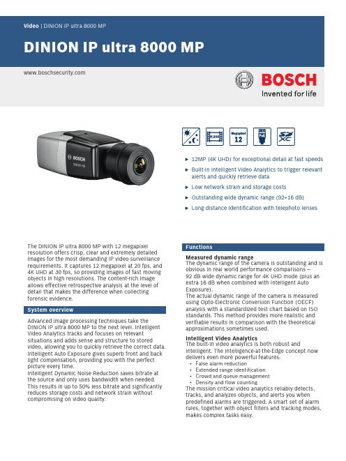
u12MP (4K UHD) for exceptional detail at fast speeds u Built-in Intelligent Video Analytics to trigger relevant alerts and quickly retrieve datau Low network strain and storage costsu Outstanding wide dynamic range (92+16 dB)u Long distance identification with telephoto lensesThe DINION IP ultra 8000 MP with 12 megapixel resolution offers crisp, clear and extremely detailedimages for the most demanding IP video surveillance requirements. It captures 12 megapixel at 20 fps, and 4K UHD at 30 fps, so providing images of fast moving objects in high resolutions. The content-rich image allows effective retrospective analysis at the level of detail that makes the difference when collectingforensic evidence.System overviewAdvanced image processing techniques take the DINION IP ultra 8000 MP to the next level. Intelligent Video Analytics tracks and focuses on relevant situations and adds sense and structure to stored video, allowing you to quickly retrieve the correct data. Intelligent Auto Exposure gives superb front and back light compensation, providing you with the perfect picture every time.Intelligent Dynamic Noise Reduction saves bitrate at the source and only uses bandwidth when needed. This results in up to 50% less bitrate and significantly reduces storage costs and network strain without compromising on video quality.FunctionsMeasured dynamic rangeThe dynamic range of the camera is outstanding and is obvious in real world performance comparisons —92 dB wide dynamic range for 4K UHD mode (plus an extra 16 dB when combined with Intelligent Auto Exposure).The actual dynamic range of the camera is measured using Opto-Electronic Conversion Function (OECF) analysis with a standardized test chart based on ISO standards. This method provides more realistic and verifiable results in comparison with the theoretical approximations sometimes used.Intelligent Video AnalyticsThe built-in video analytics is both robust and intelligent. The Intelligence-at-the-Edge concept now delivers even more powerful features:•False alarm reduction•Extended range identification•Crowd and queue management•Density and flow countingThe mission critical video analytics reliably detects, tracks, and analyzes objects, and alerts you when predefined alarms are triggered. A smart set of alarm rules, together with object filters and tracking modes, makes complex tasks easy.The system is also extremely robust and is able to reduce false alarms, for example from foliage orshaking objects, even in harsh weather conditions. The next step in video analytics is taken with theincorporation of machine learning capabilities. With Camera Trainer you can tailor the built-in Intelligent Video Analytics to detect new user-defined moving or stationary objects and situations, or any subsequent changes.Metadata is attached to your video to add sense andstructure. This enables you to quickly retrieve the relevant images from hours of stored video. Metadata can also be used to deliver irrefutable forensic evidence or to optimize business processes based on people counting or crowd density information. Intelligent Auto ExposureFluctuations in backlight and front light can ruin your images. To achieve the perfect picture in every situation, Intelligent Auto Exposure automatically adjusts the exposure of the camera. It offers superb front light compensation and incredible backlight compensation by automatically adapting to changing light conditions.Intelligent Dynamic Noise ReductionQuiet scenes with little or no movement require alower bitrate. By intelligently distinguishing between noise and relevant information, Intelligent Dynamic Noise Reduction reduces bitrate by up to 50%. Because noise is reduced at the source during image capture, the lower bitrate does not compromise on video quality.With the release of FW6.40 an extra level ofintelligence is added with Intelligent Streaming. The camera provides the most usable image possible by cleverly optimizing the detail-to-bandwidth ratio. The smart encoder continuously scans the complete scene as well as regions of the scene and dynamically adjusts compression based on relevant information like movement. Together with Intelligent Dynamic Noise Reduction, which actively analyzes the contents of a scene and reduces noise artifacts accordingly, bitrates are reduced by up to 80%. Because noise is reduced at the source during image capture, the lower bitrate does not compromise image quality. This results in substantially lower storage costs and network strain and still retain a high image quality and smooth motion.Area-based encodingArea-based encoding is another feature which reduces bandwidth. Compression parameters for up to eight user-definable regions can be set. This allows uninteresting regions to be highly compressed, leaving more bandwidth for important parts of the scene. Bitrate optimized profileThe average typical optimized bandwidth in kbits/s forvarious frame rates is shown in the table:Selectable resolution and aspect ratioThe camera has three basic application variants that can be chosen at start-up to provide the best possible performance for typical applications:•12MP (4:3)•4K UHD (16:9)•1080p (16:9)The 12MP variant can be used in applications where the highest resolution possible is required. The4K UHD variant is suitable for applications where the 16:9 4K standard is required with a frame rate of30 fps. The 1080p30 (16:9) variant is for applications that require extra sensitivity and dynamic range. Each of these variants selects the best possible tuning parameters for the application so that you get the best performance possible from your camera.Scene modesThe camera has a very intuitive user interface that allows fast and easy configuration. Nine configurable modes are provided with the best settings for a variety of applications. Different scene modes can be selected for day or night situations.Multiple streamsThe innovative multi-streaming feature delivers various H.264 streams together with an M‑JPEG stream. These streams facilitate bandwidth-efficient viewing and recording, plus easy integration with third-party video management systems.Depending on the resolution and frame rate selected for the first stream, the second stream provides a copy of the first stream or a lower resolution stream.The third stream uses the I-frames of the first stream for recording; the fourth stream shows a JPEG image at a maximum of 10 Mbit/s.Regions of interest and E-PTZRegions of Interest (ROI) can be user defined. The remote E-PTZ (Electronic Pan, Tilt and Zoom) controls allow you to select specific areas of the parent image. These regions produce separate streams for remote viewing and recording. These streams, together with the main stream, allow the operator to separately monitor the most interesting part of a scene while still retaining situational awareness.Intelligent Tracking continuously analyses the scene for moving objects. If a moving object is detected, thecamera automatically adjusts its settings, including field of view, to optimally capture details of the objectof interest.Easy installationPower for the camera can be supplied via a Power-over-Ethernet compliant network cable connection. With this configuration, only a single cable connection is required to view, power, and control the camera. Using PoE makes installation easier and more cost-effective, as cameras do not require a local power source.The camera can also be supplied with power from+12 VDC power supplies. To increase system reliability, the camera can be simultaneously connected to both PoE and +12 VDC supplies. Additionally, uninterruptible power supplies (UPS) can be used to ensure continuous operation, even during a power failure.For trouble-free network cabling, the camera supports Auto-MDIX which allows the use of straight or cross-over cables.Storage managementRecording management can be controlled by theBosch Video Recording Manager(Video Recording Manager) or the camera can use iSCSI targets directly without any recording software. Edge recordingInsert a memory card into the card slot to store up to 2 TB of local alarm recording. Pre-alarm recording in RAM reduces recording bandwidth on the network, and extends the effective life of the memory card. Cloud-based servicesThe camera supports time-based or alarm-based JPEGposting to four different accounts. These accounts can address FTP servers or cloud-based storage facilities (for example, Dropbox). Video clips or JPEG images can also be exported to these accounts.Alarms can be set up to trigger an e-mail or SMS notification so you are always aware of abnormal events.Data securitySpecial measures are necessary to ensure the highest level of security for device access and data transport. On initial setup, the camera is only accessible over secure channels. You must set a service-level password in order to access camera functions.Web browser and viewing client access can beprotected using HTTPS or other secure protocols that support state-of-the-art TLS 1.2 protocol with updated cipher suites including AES encryption with 256 bit keys. No software can be installed in the camera, and only authenticated firmware can be uploaded. A three-level password protection with security recommendations allows users to customize device access. Network and device access can be protected using 802.1x network authentication with EAP/TLS protocol. Superior protection from malicious attacks isguaranteed by the Embedded Login Firewall, on-board Trusted Platform Module (TPM) and Public KeyInfrastructure (PKI) support.The advanced certificate handling offers:•Self-signed unique certificates automatically createdwhen required•Client and server certificates for authentication •Client certificates for proof of authenticity •Certificates with encrypted private keysComplete viewing softwareThere are many ways to access the camera’s features: using a web browser, with the Bosch Video Management System, with the free-of-chargeBosch Video Client, with the video security mobileapp, or via third-party software.System integration and ONVIF conformanceThe camera conforms to the ONVIF Profile S, ONVIF Profile G and ONVIF Profile T specifications.Third-party integrators can easily access the internal feature set of the device for integration into large projects. Visit the Bosch Integration Partner Program (IPP) website () for more information.Lens optionsThe camera has a C/CS lens mount and motorized focus adjustment.There are four megapixel lenses optionally available for the camera body version, one varifocal and three fixed focal length versions:• a 4-13 mm P-iris varifocal lens (LVF-8008C-P0413)• a 35 mm fixed telephoto lens (LFF-8012C-D35)• a 50 mm fixed telephoto lens (LFF-8012C-D50)• a 75 mm fixed telephoto lens (LFF-8012C-D75)The camera body includes an auto-focus lens wizard toensure that lenses can be easily focused. The automatic motorized focus adjustment with 1:1 pixel mapping ensures that the camera with these telephoto lenses is always focused accurately.Housing optionsTo protect the camera, two housings are optionallyavailable (UHO-POE-10 and UHO-HBGS-x1). When choosing a housing keep the following in mind:• A camera with a 75 mm telephoto lens is too long for the UHO-POE-10 housing; use the UHO-HBGS-x1housing instead.DORI coverageDORI (Detect, Observe, Recognize, Identify) is astandard system (EN-62676-4) for defining the ability of a camera to distinguish persons or objects within a covered area. The maximum distance at which a camera/lens combination can meet these criteria is shown below:12MP Camera with 4-13 mm lens (29°-90°)12MP Camera with 35 mm lens (9.8°)12MP Camera with 50 mm lens (6.8°)12MP Camera with 75 mm lens (4.7°)Certifications and approvalsControlsDimensionsmm (in)Technical specificationsOrdering informationNBN-80122-CA Fixed camera 12MPHigh-performance 12 MP box cameras for intelligent 4K UHD surveillance (without lens) with audio/motion detection and motorized auto-focus.Order number NBN-80122-CAEWE-D8IPUL-IW 12mths wrty ext DINION IP ultra 8000 MP12 months warranty extensionOrder number EWE-D8IPUL-IWAccessoriesLFF-8012C-D35 Fixed lens, 35mm, telephoto, mega-pixelFixed telephoto megapixel lens ; manual iris; IR corrected; C-mount; 2/3” ; F1.8; 35mmOrder number LFF-8012C-D35LFF-8012C-D50 Fixed lens, 50mm, telephoto, mega-pixelFixed telephoto megapixel lens ; manual iris; IR corrected; C-mount; 2/3” ; F2.0; 50mmOrder number LFF-8012C-D50LFF-8012C-D75 Fixed lens, 75mm, telephoto, mega-pixelFixed telephoto megapixel lens ; manual iris; C-mount; 1/1.8” ; F1.8; 75mmOrder number LFF-8012C-D75LVF-8008C-P0413 Varifocal lens, 4-13mm, 12MP, CS mountVarifocal megapixel lens; P-iris; CS-mount; 1/1.8” ;F1.5; 4-13mmOrder number LVF-8008C-P0413NBN-MCSMB-03M Cable, SMB to BNC, camera-cable, 0.3m0.3 m (1 ft) analog cable, SMB (female) to BNC (female) to connect camera to coaxial cableOrder number NBN-MCSMB-03MNBN-MCSMB-30M Cable, SMB to BNC, camera-moni-tor/DVR3 m (9 ft) analog cable, SMB (female) to BNC (male) to connect camera to monitor or DVROrder number NBN-MCSMB-30MUPA-1220-60 Power supply, 120VAC 60Hz,12VDC 1A outPower supply for camera. 100-240 VAC, 50/60 Hz In; 12 VDC, 1 A Out; regulated.Input connector: 2-prong, North American standard (non-polarized).Order number UPA-1220-60UPA-1220-50 Power supply, 220VAC 50Hz, 12VDC 1A outPower supply for camera. 110-240 VAC, 50/60 Hz In; 12 VDC, 1 A Out; regulated.Input connector: 2-prong, European Europlug standard (4 mm / 19 mm).Order number UPA-1220-50TC9210U Camera mount, 6", indoorA universal 6-inch wall/ceiling grid with off-white finish for 4.5 kg (10 lb) max load, incl. T-Bar ceiling clip and wall/ceiling mount flange.Order number TC9210UUHO-HBGS-51 Outdoor housing, blower, 230VAC/35W Outdoor housing for (230 VAC / 12 VDC) camera with 230 VAC power supply, blower and feed-through cabling.Order number UHO-HBGS-51UHO-HBGS-61 Outdoor housing, blower, 120VAC/35W Outdoor housing for (120 VAC / 12 VDC) camera.120 VAC power supply; blower; feed-through cabling Order number UHO-HBGS-61UHO-HBGS-11 Outdoor housing, 24VAC, feed-through Outdoor housing for (24 VAC / 12 VDC) camera with 24 VAC power supply, blower and feed-through cabling.Order number UHO-HBGS-11UHO-POE-10 Outdoor housing, POE + power supply Outdoor camera housing with PoE+ power supply. Order number UHO-POE-10LTC 9215/00 Wall mount with cable feed through, 12" Wall mount for camera housing, cable feed-through, 30 cm (12 in.)Order number LTC 9215/00LTC 9215/00S Wall mount for UHI/UHOWall mount for camera housing, cable feed-through, 18 cm (7 in.)Order number LTC 9215/00SLTC 9219/01 Feed through J mountJ-mount for camera housing, 40 cm (15 in).Order number LTC 9219/01LTC 9210/01 Column mount, 8", 9KG/20lb loadFeed-through column mount for 20 cm (8 in.), 9 kg (20 lb) maximum load. Light gray finish.Order number LTC 9210/01LTC 9213/01 Pole mount adapter forLTC9210,9212,9215Flexible pole mount adapter for camera mounts (use together with the appropriate wall mount bracket). Max. 9 kg (20 lb); 3 to 15 inch diameter pole; stainless steel strapsOrder number LTC 9213/01NPD-5001-POE Power over ethernet , 15.4W, 1-port Power-over-Ethernet midspan injector for use with PoE enabled cameras; 15.4 W, 1-portWeight: 200 g (0.44 lb)Order number NPD-5001-POENPD-5004-POE Power over ethernet, 15.4W, 4-port Power-over-Ethernet midspan injectors for use with PoE enabled cameras; 15.4 W, 4-portsWeight: 620 g (1.4 lb)Order number NPD-5004-POEUPA-1220-60 Power supply, 120VAC 60Hz,12VDC 1A outPower supply for camera. 100-240 VAC, 50/60 Hz In; 12 VDC, 1 A Out; regulated.Input connector: 2-prong, North American standard (non-polarized).Order number UPA-1220-60ServicesEWE-D8IPUL-IW 12mths wrty ext DINION IP ultra 8000 MP12 months warranty extensionOrder number EWE-D8IPUL-IWRepresented by:Europe, Middle East, Africa:Germany:North America:Asia-Pacific:Bosch Security Systems B.V.P.O. Box 800025600 JB Eindhoven, The Netherlands Phone: + 31 40 2577 284****************************** Bosch Sicherheitssysteme GmbHRobert-Bosch-Ring 585630 GrasbrunnGermanyBosch Security Systems, Inc.130 Perinton ParkwayFairport, New York, 14450, USAPhone: +1 800 289 0096Fax: +1 585 223 9180*******************.comRobert Bosch (SEA) Pte Ltd, Security Systems11 Bishan Street 21Singapore 573943Phone: +65 6571 2808Fax: +65 6571 2699*****************************© Bosch Security Systems 2019 | Data subject to change without notice 12540006027 | en, V35, 25. Nov 2019。
management企业管理类英文版
Processes-SupportedCount BP-Risk-AverageInherent Materiality-I-Count Materiality-G-Count Materiality-S-Count IT Tier
KLS Consulting LLC
ITRA
ADOS Risk Factors
Risk Enterprise Risk Mgt (COSO, COCO)
Operational Risk Mgt
IT Risk Mgt (CobiT, ITIL, etc.)
Compliance
Public Companies (Sarbanes-Oxley, NYSE, Nasdaq, Turnbull, etc.)
Management should:
Evaluate whether it has implemented controls that adequately address the risk that a material misstatement of the financial statements would not be prevented or detected in a timely manner.
Outsourcer-SAS 70 Report Opinion, Testing Exceptions-Moderate, & Testing Exceptions-Major
App Server OS-VendorReputation
DB Server OS-VendorReputation
App Server OS-VersionSupported
精选课件
KLS Consulting LLC
NI PXI-6602
C o u n t e r /T i m e r O v e r v i e wD a t a A c q u i s i t i o n a n d S i g n a l C o n d i t i o n i n gYou can use the versatile National Instruments counter/timer devices to create a wide variety of measurement solutions,including measuring a number of time-related quantities,counting events or totalizing,and monitoring position with quadrature encoders.You can also use counter/timers to generate pulses and pulse trains.Counter/timers often fulfill critical timing functions as components of complex measurement systems.The NI 660x counter/timers use the NI-TIO, a National Instruments AS IC chip specifically designed to meet the counting and timing requirements of measurement applications that are beyond the capabilities of off-the-shelf components.The wider functionality and simple programming interface make the NI 660x your best choice for counting and timing applications.Example applications include frequency measurement,position measurement,generation of retriggerable pulses,frequency shift-keying,two-signal edge separation measurements,continuous buffered event counting,and continuous buffered pulse train measurements.The NI 660x counter/timer devices are readily integrated into measurement systems that require synchronization across multiple hardware devices because they are equipped with the National Instruments PXI trigger bus or the RTS I bus.S ee the counter/timer tutorial on page 789 for more information.In addition to counter/timer functionality,the NI 660x products include TTL/CMOS -compatible digital I/O ports that are bit configurable for input or output.Counter/Timer ConsiderationsNumber of Counter/TimersThe counter/timer is a basic unit of hardware functionality on a measurement device.The more counter/timers there are on a device,the more counting/timing operations that device can simultaneously perform.The number of DMA channels determines how many buffered,high-speed operations can be simultaneously performed.See page 393 for more information.Counter/Timer Size or Number of BitsThe counter size or number of bits indicates how high a counter can count.For example,a 32-bit counter can count up to 232-1 or 4,294,967,295 before it rolls over.A high number of bits is beneficial in cases such as pulse width measurements where a wide dynamic range is required.For example,if you measure pulse widths with a 12.5 ns resolution (80 MHz timebase) using a counter/timer with 32 bits,you can measure pulse widths up to 53 s [(232-1) x 12.5 ns)]with 12.5 ns resolution.Maximum Source FrequencyMaximum source frequency represents the speed of the fastest signal the counter can count.If you use a higher source frequency,you can achieve higher resolution.For example,an 80 MHz counter can count pulses that are 12.5 ns (1⁄80 x 106) apart.You can use prescalers to increase the maximum source frequency for event counting and frequency measurement.Counter/Timer OverviewDebouncing/Counter/Max SourcePulse Buffered Glitch Oscillator GPSBuffered Operations 2Family Bus Timers Size Frequency Compatibility Digital I/O GenerationOperationsRemoval Stability Synchr.DMA Interrupt PageNI 6601PCI 432 bits 20 MHz 1 5 V TTL/CMOS Up to 32✓✓✓50 ppm –13388NI 6602PCI 832 bits 80 MHz 1 5 V TTL/CMOS Up to 32✓✓✓50 ppm–35388PXI NI 6608PXI832 bits80 MHz 15 V TTL/CMOSUp to 32✓✓✓75 ppb✓353881Max Source Frequency with prescalers is 60 MHz for the NI 6601 and 125 MHz for the NI 6602 and NI 6608. These frequencies are dependent on drive strength of input signal and cable length. Consider these speeds to be the maximum. 2DMA transfers have higher throughput than interrupt transfers. See page 393 for detailed specifications.Counter/Timer OverviewCounter/Timer OverviewSignal CompatibilitySignal compatibility indicates the signal levels a counter/timer can measure or output,such as TTL/CMOS.Buffered Operations and DMAThe National Instruments counter/timers can capture numerous data points without dead times.These types of measurements,called buffered operations,are valuable in applications that range from statistical analysis on production lines to experiments in molecular chemistry.For instance,when you configure a counter for buffered period measurement,data is moved from the counter into a buffer.Each edge that initiates a measurement also causes a transfer of the count into the buffer,as shown in Figure 1.With buffered operations,data is transferred to the computer memory using DMA or interrupts.DMA offers a considerable performance advantage;if your application requires this performance simultaneously on multiple counter/timers,you must know how many DMA channels are available on a particular counter/timer device.For example,if a device contains three DMA channels and eight counter/timers,you can simultaneously perform three high-speed and five lower-speed,interrupt-based,buffered operations.On NI 660x devices,National Instruments implements DMA with the NI MITE chip,which is optimized for measurement applications.Timebase StabilityTimebase stability can be important when you need to make high-quality measurements.Crystal oscillators typically form the basis of electrical circuits used to drive timing of a measurement application.In an ideal case,the oscillation frequency would be constant,but in reality,many factors influence the the behavior of an oscillator.A commonly used measure of quality for an oscillator is stability.Units used for stability are typically parts per million (ppm) and parts per billion (ppb).For example,the frequency of a 10 MHz oscillator with 10 ppm stability can be 10 MHz ±100 Hz;with 100 ppb stability it can be 10 MHz ±1 Hz.The best technique for improving oscillator stability is to precisely control its temperature as is done in an oven-controlled crystal oscillator (OCXO).The PXI-6608 features such an oscillator.Debouncing and Glitch RemovalNoisy signals containing glitches and/or bouncing effects pose special challenges for some counter/timer measurements.Noise may be introduced in the source of the signal,such as with electromechanical relays,or in the connection if there are strong sources of interference in the vicinity of the system.NI 660x devices contain programmable digital filters that eliminate measurement errors caused by spurious spikes and bouncing.Figure 2 shows an example of digital filtering.CalibrationCalibration is a key component of any measurement solution.In the case of counter/timers,timebase calibration ensures that the frequency and time measurements are accurate.Calibration certificates enclosed with the National Instruments counter/timers and periodic calibration satisfy your IS O-9000 requirements,certifying that your instrument has been properly calibrated.S ee page 21 for more information.32-B i t C o u n t e r /T i m e r sD a t a A c q u i s i t i o n a n d S i g n a l C o n d i t i o n i n gOverview and ApplicationsNI 660x devices are timing and digital I/O (DIO) modules for PCI and PXI.They offer up to eight 32-bit counter/timers and up to 32 lines of 5 V TTL/CMOS-compatible digital I/O.You can perform a wide variety of buffered measurements or other counter/timer tasks with NI 660x devices,including position or quadrature encoder measurement,event counting,period measurement,pulse-width measurement,frequency measurement,pulse generation,and pulse-train generation.Features Counter/Timers The NI 660x devices are equipped with the NI-TIO ASIC, a National Instruments counter and digital I/O ASIC for advanced timing and counting applications.Each NI 6602 and NI 6608 device features two NI-TIO ASICs to provide a total of eight counter/timers.The PCI-6601 board features one NI-TIO ASIC for a total of fourcounter/timers.The counters are software-compatible with those found on E Series multifunction DAQ devices,but NI 660x devices offer additional capabilities.Each counter has a gate,up/down,and source signal,which can be controlled by external or internal signals.Each counter has one output that can be routed externally or to other counters on the device.20 MHz and 100 kHz timebases are available on each device for use with each counter/timer.In addition,an 80 MHz timebase isavailable on the NI 6602 and NI 6608 devices.A hardware trigger canbe used to start multiple counters simultaneously.See Table 1 for more information.•Up to eight 32-bit counter/timers •80 MHz maximum source frequency (125 MHz with prescalers)•Debouncing and glitch removal •High-stability timebase (PXI-6608 only)•GPS-based synchronization (PXI-6608 only)•NI DAQ driver simplifiesconfiguration and measurementsModels•NI PCI-6601•NI PCI-6602•NI PXI-6602•NI PXI-6608Operating Systems•Windows 2000/NT/XP •Real-time performance with LabVIEW (p.134)•Others such as Linux and Mac OS X (page 187)Recommended Software•LabVIEW•LabWindows/CVI •Measurement Studio Other Compatible Software •Visual Basic•Visual C/C++,C#Driver Software (included)•NI-DAQ 7Calibration Certificate IncludedSee page 21.NI 660x32-Bit Counter/TimersDebouncing/Counter/Max Source Pulse Buffered Glitch Oscillator GPSBuffered Operations 2FamilyBus Timers Size Frequency Compatibility Digital I/O GenerationOperationsRemoval Stability Synchr.DMA Interrupt NI 6601PCI 432 bits 20 MHz 1 5 V TTL/CMOS Up to 32✓✓✓50 ppm –13NI 6602PCI 832 bits 80 MHz 1 5 V TTL/CMOS Up to 32✓✓✓50 ppm–35PXI NI 6608PXI832 bits80 MHz 15 V TTL/CMOSUp to 32✓✓✓75 ppb✓351Max Source Frequency with prescalers is 60 MHz for the NI 6601 and 125 MHz for the NI 6602 and NI 6608. These frequencies are dependent on drive strength of input signal and cable length. Consider these speeds to be the maximum. 2DMA transfershave higher throughput than interrupt transfers.Table 1. NI 660x Products Specifications Summary (See page 393 for detailed specifications.)32-Bit Counter/Timers32-Bit Counter/TimersData Acquisition and Signal ConditioningHigh-Stability, Oven-Controlled OscillatorThe NI PXI-6608 module includes a high-stability 10 M Hz oven-controlled crystal oscillator (OCXO) for high-precision applications.When the PXI-6608 is installed in the star trigger slot of a PXI chassis (Slot 2),you can drive the OCXO signal to the PXI backplane for high-stability timing of your entire measurement system.The PXI-6602 and PXI-6608 feature phase-lock loop (PLL)circuitry so that the devices can synchronize their reference clocks to the backplane.Debouncing and Glitch RemovalEach input on the NI 660x devices can be passed through a digital debouncing filter to eliminate glitches on the input signal.You can use defined filter settings to remove noise/glitches narrower than 2.5 µs,500 ns,250 ns,and 50 ns from your input signal,or you can use one of the counters to create custom filter settings.Buffered MeasurementsNI 660x devices use the National Instruments MITE bus interface controller to implement bus-master DM A transfers.As a result,you can perform high-speed,continuous operations such as buffered position encoder measurement and buffered period measurement.You can perform one high-speed DM A-based transfer on the NI 6601 devices and up to three simultaneous DMA transfers on the NI 6602 and NI 6608 devices.You can use interrupts for additional simultaneous buffered transfers.Digital I/ONI 660x devices.dedicated to DIO,or output.RTSI Bus and PXI Trigger Bussynchronization.synchronization.Synchronizing Networked Measurements with GPSYou can correlate measurements performed in a wide area using the Global Positioning System (GPS).With the PXI-6608,you can correlate data from several PXI chassis,determine the time when a hardware event occurs,or generate a pulse at a user-specified time.I/O ConnectorThe NI 660x devices each have a 68-pin shielded,latching connector,with a SOURCE,GATE,UP/DOWN,and OUT signal for each of the counter/timers.PFI<8..31> can be used as general-purpose DIO lines when not used as counter/timer I/O signals.The DIOn lines are the eight dedicated DIO lines.The PCI-6601 devices have the same I/O interface,except that only counters 0-3 are present.Driver SoftwareWith NI-DAQ driver software,you can configure your devices interactively,write custom programs,and perform counter/timer I/O easily.NI-DAQ provides the counter/timer functions natively,so you can programmatically select whether you want to measure position with a quadrature encoder,measure a frequency,output a pulse train,or perform one of the other provided counter/timer functions.NI-DAQ also includes numerous example programs for LabVIEW and other ADEs to quickly get you started with your application.Figure 1. NI 660x I/O ConnectorC o u n t e r /T i m e r A c c e s s o r i e s a n d C a b l e sD a t a A c q u i s i t i o n a n d S i g n a l C o n d i t i o n i n gAccessory and Cable Selection ProcessStep 1.Select your counter/timer device from Tables 1 and 2.Step ing Tables 1 and 2 as a guide,determine which accessories are appropriate for that device.Select an accessory using Table 3 as reference.Step ing Tables 1 and 2,determine the appropriate cable solution for your selected counter/timer device and accessory.AccessoriesBNC-2121 (See Figure 1)Connector block with BNC and spring terminal connections for easy connection of I/O signals to counter/timer devices.The BNC-2121 offers spring terminals,as well as eight dedicated and six user-defined BNC connectors,which provide access to all I/O signals.This connector block is also a full-featured test accessory that provides pulse-train,trigger,and quadrature encoder signals.For the connections,refer to the BNC-2121 user guide at /manualsBNC-2121......................................................................................................778289-01Dimensions – 26.7 by 11.2 by 5.5 cm (8.0 by 4.4 by 2.2 in.)CA-1000 (See Figure 2)Configurable signal connectivity solution for connecting counter/timers to different types of standard I/O connectors.You can also incorporate switches and LED indicators.You can place the CA-1000 under a laptop PC,on a benchtop,or in a 19 in.rack.CA-1000......................................................................................................See page 351Dimensions – 30.7 by 25.4 by 4.3 cm (12.1 by 10 by 1.7 in.)Counter/Timer Accessories and CablesFigure 2. CA-1000 Configurable Signal Conditioning SolutionFigure 1. BNC-2121 Connector BlockAccessory DescriptionPage BNC-2121BNC connector block with built-in test features390CA-1000Configurable connector accessory 390SCB-68Shielded screw connector block 391TB-2715Front-mount terminal block for PXI-660x391TBX-68DIN-rail connector block 391CB-68LP Low-cost screw connector block 391CB-68LPR Low-cost screw connector block 391Table 1. Accessories and Cables for PXI-6601 and PCI-6602Table 2. Accessories and Cables for PXI-6602 and PXI-6608Table 3. Overview of AccessoriesPCI-6601, PCI-6602AccessoriesCables BNC-2121, CA-1000, SCB-68,–TBX-68, CB-68LP , and CB-68LPR R6868 or SH68-68-D1TB-2715N/APXI-6602, PXI-6608AccessoriesCables BNC-2121, CA-1000, SCB-68,–TBX-68, CB-68LP , and CB-68LPR R6868 or SH68-68-D1TB-2715Connects directly to the deviceCounter/Timer Accessories and CablesSCB-68 Shielded I/O Connector Block (See Figure 3)Shielded I/O connector block for easy connection of I/O signals to the counter/timer devices.T he screw terminals are housed in a metal enclosure for protection from noise bined with a shielded cable,the SCB-68 provides rugged,very low-noise signal termination.T he SCB-68 also includes two general-purpose breadboard areas.SCB-68..............................................................................................................776844-01 Dimensions – 19.5 by 15.2 by 4.5 cm (7.7 by 6.0 by 1.8 in)TB-2715 Terminal Block (See Figure 4)With the T B-2715 terminal block for PXI counter/timer devices,you can connect signals directly without additional cables.Screw terminals provide easy connection of I/O signals.The TB-2715 latches to the front of your PXI module with locking screws and provides strain relief.TB-2715............................................................................................................778242-01 Dimensions – 8.43 by 10.41 by 2.03 cm (3.32 by 4.1 by 0.8 in.)TBX-68 I/O Connector Block with DIN-Rail Mounting (See Figure 5) Termination accessory with 68 screw terminals for easy connection of field I/O signals to the counter/timer devices.The TBX-68 is mounted in a protective plastic base with hardware for mounting on a standard DIN rail.TBX-68..............................................................................................................777141-01 Dimensions – 12.50 by 10.74 cm (4.92 by 4.23 in.)CB-68LP and CB-68LPR I/O Connector Blocks (See Figure 6)Low-cost termination accessories with 68 screw terminals for easy connection of field I/O signals to the counter/timer devices.The connector blocks include standoffs for use on a desktop or mounting in a custom panel.T he CB-68LP has a vertically mounted 68-pin connector.The CB-68LPR has a right-angle mounted connector for use with with the CA-1000.CB-68LP............................................................................................................777145-01 Dimensions – 14.35 by 10.74 cm (5.65 by 4.23 in.)CB-68LPR........................................................................................................777145-02 Dimensions – 7.62 by 16.19 cm (3.00 by 6.36 in.)Counter/Timer Accessories and CablesData Acquisition andSignal ConditioningFigure 6. CB-68LP and CB-68LPR I/O Connector BlocksFigure 5. TBX-68 I/O Connector BlockFigure 4. TB-2715 I/O Terminal BlockFigure 3. SCB-68 Shielded I/O Connector BlockC o u n t e r /T i m e r A c c e s s o r i e s a n d C a b l e sD a t a A c q u i s i t i o n a n d S i g n a l C o n d i t i o n i n gCablesRTSI Bus Cables (See Figures 7 and 8)Use RT SI bus cables to connect timing and synchronization signals among measurement,vision,motion,and CAN boards for PCI.For systems using long and short boards,order the extended RTSI cable.2 boards ..........................................................................................................776249-023 boards ..........................................................................................................776249-034 boards ..........................................................................................................776249-045 boards ..........................................................................................................776249-05Extended,5 boards ........................................................................................777562-05SH68-68-D1 Shielded Cable (See Figure 9)Shielded 68-conductor cable terminated with two 68-pin female 0.050 series D-type connectors.This cable connects counter/timer devices to accessories.1 m..................................................................................................................183432-012 m..................................................................................................................183432-02R6868 Ribbon I/O Cable (See Figure 10)68-conductor flat ribbon cable terminated with two 68-pin e this cable to connect the NI PCI-6601 to an accessory.For signal integrity with high-frequency signals,use the SH68-68-D1 with the NI 6602 and NI 6608.1 m..................................................................................................................182482-01Custom Connectivity Components68-Pin Custom Cable Connector/Backshell Kit (See Figure 11)68-pin female mating custom cable kit for use in making custom 68-conductor cables.Solder-cup contacts are available for soldering of cable wires to the connector.68-pin custom cable kit ................................................................................776832-01PCB Mounting ConnectorsPrinted circuit board (PCB) connectors for use in building custom accessories that connect to 68-conductor shielded and ribbon cables.Two connectors are available,one for right-angle and one for vertical mounting onto a PCB.68-pin,male,right-angle mounting..............................................................777600-0168-pin,male,vertical mounting....................................................................777601-01Counter/Timer Accessories and CablesFigure 10. R6868 Ribbon I/O CableFigure 9. SH68-68-D1 Shielded CableFigure 8. Extended RTSI Bus CableFigure 7. RTSI Bus CableFigure 11. 68-Pin Custom Cable KitThese specifications are typical for 25 °C unless otherwise noted.Timing I/OGeneral-Purpose Up/Down Counter/TimersNumber of channelsNI 6601...................................................... 4 up/down counters NI 6602/6608.............................................8 up/down counters Counter size/number of bits.............................32 bitsPrescalers (per counter)...................................3 bits (divided by 8) 1 bit (divided by 2)Disabled (by default)Power-on state.................................................Input (high-Z), pulled lowPull down current: 10 µA (min) to 200 µA (max)Hysteresis.........................................................300 mV Schmitt triggers Compatibility.................................................... 5 V TTL/CMOSDigital logic levelsBase clocks availableNI 6601......................................................100 kHz and 20 MHzNI 6602/6608.............................................100 kHz, 20 MHz, and 80 MHz Base clock accuracy (NI 6601 and NI 6602)....±0.005% (50 ppm)1Base clock (OCXO) accuracy (NI 6608).............±0.0000075% (75 ppb)Maximum source frequencyExternal source selections...............................I/O connector, RTSI/PXI Trigger lines, software selectable External gate selections...................................I/O connector, RTSI/PXI Trigger lines, software selectable 1 If a PXI-6608 is installed in slot 2 of a PXI chassis, then the PXI-6608 and any PXI-6602installed in that chassis inherit a base clock accuracy of ±0.0000075% (75 ppb).Minimum source pulse durationWith prescalers......................................... 3.5 ns; edge-detect mode Without prescalers.................................... 5 ns; edge-detect mode Minimum gate pulse duration.......................... 5 ns; edge-detect mode Frequency ranges to measure or generateData TransfersTransfer modes.................................................DMA, interrupts, programmed I/OTransfer ratesDMA channelsNI 6601......................................................1NI 6602/6608 (3)Oven-Controlled Crystal Oscillator (OCXO)(NI 6608 Only)Frequency.........................................................10 MHzOCXO accuracy.................................................±0.0000075% (75 ppb)Warm-up time (to within 0.02 ppmof operating frequency)............................. 5 minutesFrequency stability versussupply voltage change (±5%)....................≤0.005 ppm Temperature stability (0 to 50 °C)....................≤0.005 ppmDrift in frequency.............................................≤0.00045 ppm/day ≤0.045 ppm/yearAllowed frequency adjustment........................0.5 ppm, typicalNote: You can use the OCXO to replace the PXI 10 MHz backplane clock when the PXI-6608 is installed in the PXI star trigger slot (Slot 2). You can also use it as the counter source or gate in any slot.Digital I/ONumber of channels.........................................Up to 32 input/output Compatibility.................................................... 5 V TTL/CMOSPower-on state.................................................Input (high-Z), pulled low Pulldown current..............................................10 µA (min) to 200 µA (max)Hysteresis.........................................................300 mV Schmitt triggers Data transfers..................................................Unstrobed I/ODigital logic levelsRTSI Bus (PCI Only)Trigger lines......................................................7Minimum pulse widthfor trigger and clock..................................25 nsPXI Trigger Bus (PXI Only)Trigger lines......................................................6Star trigger. (1)Bus InterfacePCI, PXI.............................................................Master, slavePower RequirementsPhysicalDimensions (not including connectors)PCI..............................................................17.5 by 9.9 cm (6.9 by 3.9 in.)PXI..............................................................16.0 by 10.0 cm (6.3 by 3.9 in.)I/O connector....................................................68-pin male SCSI-II typeEnvironmentOperating temperature.....................................0 to 50 °C Storage temperature........................................-20 to 70 °CRelative humidity.............................................10 to 90%, noncondensingCertifications and CompliancesCE Mark ComplianceCounter/Timer SpecificationsCounter/Timer SpecificationsData Acquisition and Signal ConditioningSpecificationsLevelMinimum Maximum Input low voltage -0.3 V 0.8 V Input high voltage2.0 V 5.25 V Output low voltage (I out = 4 mA)–0.4 V Output high voltage (I out = 4 mA)2.4 V–Family Without PrescalingWith PrescalingNI 660120 MHz 60 MHz NI 660280 MHz 125 MHz NI 660880 MHz125 MHzFamily Frequency to MeasureMin/Max Frequency to GenerateNI 660120 MHz 10 MHz NI 660280 MHz 40 MHz NI 660880 MHz40 MHzFor more information, please visit /info and enter exatzz.Continuous Operation Continuous OperationBuffer Size (MS)Rate (kS/s)Buffer Size (kS)Rate (kS/s)50285015DMA 1,2Interrupt 1,3Finite Operation Finite Operation Buffer Size (S)Rate (MS/s)Buffer Size (S)Rate (kS/s)100 5.0100551,000 4.21,0004910,000 2.010,00049100,000 1.8100,000481Values may vary depending on your computer hardware, operating system and systemactivity. Benchmark data was determined on a Pentium II 400 MHz computer with 64 MB RAM running Windows 98 and LabVIEW using one counter of a PCI-6602. 2The number of simultaneous DMA transfers you can perform is equivalent to the DMA channels available on your device. 3The rate is based on one counter using the interrupts. If multiple counters share interrupts, the transfer rate per counter is lower.LevelMinimum Maximum Input low voltage -0.3 V 0.8 V Input high voltage2.0 V 5.25 V Output low voltage (I out = 4 mA)–0.4 V Output high voltage (I out = 4 mA)2.4 V–Device +5 VDC (±5%)*Power Available at I/O ConnectorNI 66010.4 to 0.75 A +4.65 to +5.25 VDC, 1 A NI 66020.5 to 1.5 A +4.65 to +5.25 VDC, 1 A NI 66081 to 2.5 A+4.65 to +5.25 VDC, 1 A*Excludes power consumed through I/O connectorC o u n t e r /T i m e r O v e r v i e wD a t a A c q u i s i t i o n a n d S i g n a l C o n d i t i o n i n gYou can use the versatile National Instruments counter/timer devices to create a wide variety of measurement solutions,including measuring a number of time-related quantities,counting events or totalizing,and monitoring position with quadrature encoders.You can also use counter/timers to generate pulses and pulse trains.Counter/timers often fulfill critical timing functions as components of complex measurement systems.The NI 660x counter/timers use the NI-TIO, a National Instruments AS IC chip specifically designed to meet the counting and timing requirements of measurement applications that are beyond the capabilities of off-the-shelf components.The wider functionality and simple programming interface make the NI 660x your best choice for counting and timing applications.Example applications include frequency measurement,position measurement,generation of retriggerable pulses,frequency shift-keying,two-signal edge separation measurements,continuous buffered event counting,and continuous buffered pulse train measurements.The NI 660x counter/timer devices are readily integrated into measurement systems that require synchronization across multiple hardware devices because they are equipped with the National Instruments PXI trigger bus or the RTS I bus.S ee the counter/timer tutorial on page 789 for more information.In addition to counter/timer functionality,the NI 660x products include TTL/CMOS -compatible digital I/O ports that are bit configurable for input or output.Counter/Timer ConsiderationsNumber of Counter/TimersThe counter/timer is a basic unit of hardware functionality on a measurement device.The more counter/timers there are on a device,the more counting/timing operations that device can simultaneously perform.The number of DMA channels determines how many buffered,high-speed operations can be simultaneously performed.See page 393 for more information.Counter/Timer Size or Number of BitsThe counter size or number of bits indicates how high a counter can count.For example,a 32-bit counter can count up to 232-1 or 4,294,967,295 before it rolls over.A high number of bits is beneficial in cases such as pulse width measurements where a wide dynamic range is required.For example,if you measure pulse widths with a 12.5 ns resolution (80 MHz timebase) using a counter/timer with 32 bits,you can measure pulse widths up to 53 s [(232-1) x 12.5 ns)]with 12.5 ns resolution.Maximum Source FrequencyMaximum source frequency represents the speed of the fastest signal the counter can count.If you use a higher source frequency,you can achieve higher resolution.For example,an 80 MHz counter can count pulses that are 12.5 ns (1⁄80 x 106) apart.You can use prescalers to increase the maximum source frequency for event counting and frequency measurement.Counter/Timer OverviewDebouncing/Counter/Max SourcePulse Buffered Glitch Oscillator GPSBuffered Operations 2Family Bus Timers Size Frequency Compatibility Digital I/O GenerationOperationsRemoval Stability Synchr.DMA Interrupt PageNI 6601PCI 432 bits 20 MHz 1 5 V TTL/CMOS Up to 32✓✓✓50 ppm –13388NI 6602PCI 832 bits 80 MHz 1 5 V TTL/CMOS Up to 32✓✓✓50 ppm–35388PXI NI 6608PXI832 bits80 MHz 15 V TTL/CMOSUp to 32✓✓✓75 ppb✓353881Max Source Frequency with prescalers is 60 MHz for the NI 6601 and 125 MHz for the NI 6602 and NI 6608. These frequencies are dependent on drive strength of input signal and cable length. Consider these speeds to be the maximum. 2DMA transfers have higher throughput than interrupt transfers. See page 393 for detailed specifications.。
Real-Time Kernel in Hardware RTU A step towards deterministic and high performance real-tim
Real-Time Kernel in Hardware RTU:A step towards deterministic and high performance real-time systemsJoakim Adomat, Johan Furunäs, Lennart Lindh, Johan StärnerMälardalens University, IDT/ Department of Real-Time Computer Systemsemail: lennart.lindh@mdh.se, joakim.adomat@mdh.se, johan.starner@mdh.se, johan.furunas@mdh.seAbstractDemands on real-time kernels increase every year: as applications grow larger and become more complex, real-time kernels must give short and predictable response.The RTU is a real-time kernel coprocessor implemented in an ASIC, which is intended to meet the growing expectations on real-time kernels.Since the RTU gives fast response times, it is necessary to define a detailed time-model to improve the understanding of the real-time kernel behaviour in the µS-domain.In this paper, we describe how to use the RTU in a single - or multi-processor architecture and a time-model for a RTU based real-time system is defined. The time-model is considered with regards to determinism and performance. Keywords: determinism, performance, Real-Time system, Real-Time kernel.1. IntroductionIn this article we describe the RTU (Real Time Unit) [1] and analyse the time behaviour in a Real-Time system without application software. The motivation is to understand the increasing performance and determinism in the system by using a RTU.An exact time analysis of a system is often not possible, because of lack of information and the usually big gap between best and worst case response time in the real-time kernel. The gap can be seen as a measure of determinism.The determinism and performance can be improved by implementing the kernel in hardware, e.g. the RTU. But when a kernel like RTU is used, with response times below 1µs, the overhead time from buses, hardware arbitration, hardware interrupt latency, etc. is no longer negligible. This requires a more exact time-model to give a better understanding of the system behaviour. The time-model in this article is used to make the behaviour of a real-time system, based on a bus with processors without application tasks, easier to understand.The RTU is a small single - or multiprocessor multitasking real-time kernel implemented in hardware. It can handle a maximum of 64 tasks at 8 priority levels, which can be mapped onto up to three CPUs. The RTU consists of a number of units (see figure 1) which handles the different kernel functions i.e. wait for next period, delay, semaphore, event flag, watchdog, interrupt, local -and global scheduling (priority preemptive), activation and termination of tasks. The interface to the RTU is read- and writeable registers, which makes it easy to port it to different types of processors. Furthermore the RTU ASIC (Application Specific Integrated Circuit) is now tested and working. With an on chip external communication protocol it is possible to change or add kernel functionality by mapping functions onto FPGAs (Field Programmable Gate Array) outside the RTU. When the changes/add-ons are tested they can be incorporated in the next RTU-generation. The RTU is designed with a lot of true concurrent running parts and that is the solution toget response times [5] within the µs domain.Figure 1. Internal structure of the RTU.2 System architecture with the RTUThe RTU is currently configured to operate on a bus-based, task-level parallel (i.e. tasks are executed in parallel) single - and multiprocessor system.Since the communication with the RTU is register based it is possible to have different application processors executing in the system.Our research system is VME [3] bus based. It is currently configured (see figure 2) with a RTU, up to three Force 68010 CPU-3VA [2], a global memory and a bus arbiter mapped onto a FPGA. The RTU can handle up to 3 application processors. Each application processor must be configured to respond to a specific VME interrupt, which the RTU drives to inform the CPU to perform a task switch, i.e. interrupt lines 0 - 2 in figure 2.To be able to calculate the maximum access time for each CPU, in a multi processor system, a round-robin arbiter is used to control the accesses to the bus. A priority basedbus arbiter can not guarantee the worst case time.Figure 2. A real-time system based on the RTU2.1 Interface to the RTUThe communication between the RTU and the application processors is done with interrupts, reading and writing in registers. The communication is often done in 4-6 bus accesses to the registers. For more information about the RTU interface see [6].A short description of each RTU register: CPU STATUS REGISTER. Consists of three registers, one for each CPU. It holds the status of its respective CPU ,e.g. context switch is enabled on a CPU.RTU STATUS REGISTER. Holds the RTU status, e.g. perform a service which is received from a CPU.RTU CONTROL REGISTER. Controls the timer which is used for on chip time functions, e.g. delay, periodic start and watch dogs.NEXT TASK ID. Consists of three registers, one for each CPU. It holds the running task id for each CPU.SVC INSTRUCTION REGISTER. Consists of three registers, one for each CPU. The service calls are written to the register. A service call is e.g. wait for a semaphore. CPU CONTROL REGISTER. Consists of three registers, one for each CPU. It controls CPU related functions e.g. disable context switch on a CPU and reschedule a new task.The RTU registers can be accessed directly from the CPU. No semaphore is needed because no shared registers are used between the CPUs. However the CPU must block task-switch when it performs a service call, because the SVC INSTRUCTION REGISTER is shared between the tasks on one processor.If a task wants to perform a service call (see protocol below) e.g. wait for next period, it must write the service call to the SVC INSTRUCTION REGISTER. To request a new task for a CPU, the CPU must write to its CPU CONTROL REGISTER.The protocol for a service call in a single or multiprocessor system is described below:1. Write disable context switch to the CPU CONTROL REGISTER.2. Write service call to SVC INSTRUCTION REGISTER.3. Read RTU STATUS REGISTER to check if the RTU received the service call.4. Write the end of service call code to SVC INSTRUCTION REGISTER to inform the RTU to start the service.5. Read RTU STATUS REGISTER to check if the RTU is ready with the service. Continue the read until the RTU is ready with the service. Since the RTU is fast, the CPU never has to wait for ready service.6. Write enable context switch to CPU CONTROL REGISTER.Step 3 and 5 are handshake actions, to make the communication with the RTU more reliable. The motivation for having handshake signals is to discover any disturbances in the system, e.g. a glitch on the VME bus.3 Performance and determinism analysisIn this section an accurate time model for real-time system based on the RTU (see figure 2) with cache-less CPUs is defined and discussed with respect to determinism and performance. In the discussion, a comparison with software kernels (SWK) is done. The time models based on the software kernels are just estimated, since it is hard to find information about how they work.To be able to define an accurate time model for a real-time system based on the RTU, the time consuming parts in the system, i.e. time not spent on executing tasks, must be defined. The following parts are defined to consume time, in our model of a real-time system:-Service calls: The service call time can be defined as T servicecall= T i/o+T service. T i/o is the interface time between the CPU and the RTU and T service is the time the RTU uses to perform a service. Since T i/o consists of m numbers of bus accesses it can be defined asT i/o=m*(T read/write+T busmax+T arbitration). m is the number of bus accesses. T read/write is the time for an absolute read or write instruction. T busmax is the maximum bus waiting time for the bus i.e. a CPU must wait on n numbers of CPUs to be ready with their bus accesses. T arbitration is the arbitration time, which is algorithm dependent, in this case it is a round-robin arbiter. T busmax=(n-1)*(T arbitration+T read/write). n is the number of CPUs.-Task switch: The task switch time can be defined as T taskswitch=T busmax+T irq+T getnexttask+T changeregs+T rte. T irq is the interrupt time on a CPU i.e. saving program counter and status registers to the stack. T changeregs is the time which the CPU spent on saving registers for the old task and restoring registers for the new task. T busmax stands for the waiting time on the bus during the interrupt process. T rte is the return from interrupt time i.e. restoring status registers and the program counter from stack. Since T getnexttask is one bus access to the RTU NEXT TASK ID register, it can be defined as T getnexttask=T read/write+T busmax+T arbitration.-Clock tick administration: The clock tick administration time can be defined as T clocktick=T irq+T adb+T rte. T adb is the time spent on updating task queues and scheduling i.e. T scheduling.-Scheduling: The scheduling time is the time it takes to schedule tasks and is defined as T scheduling3.1 Clock tick administration on a CPUIn a real-time system there exists different task queues, e.g. time queues and resource queues, which must be updated. To start the kernel in a real-time system, a timer is used to periodically generate clock tick interrupts. However when a RTU is used, all updating of time queues are performed within the RTU. Therefore the CPU does not have to be interrupted by clock ticks which means that T clocktick=0 when the real-time kernel is a RTU. In the SWK e.g. pSOS[4] case where the real-time kernel is located on the CPU T clocktick=T irq+T adb+T rte. Determinism:The administration time usually varies a lot in the software kernel case since the different time - and task queues alter dynamically when the system is running. The search times on the queues changes because of the alternating length of the queues, which decrease the determinism.Performance:The higher the tick frequency gets the better the granularity, but the time spent on executing tasks decreases. With a low tick time, the tick frequency can be high with a maintained large utilization factor on the CPU. When a RTU is used as a kernel, the CPUs don’t need clock-tick administration which gives more system capacity left to execute application tasks.3.2 Service callOne of the real-time kernel’s jobs is to serve tasks with different services e.g. semaphore handling. When a service call is performed by the RTU, the service call time T servicecall is only dependent on how much time T i/o consumes since T service is negligible compared to T i/o. In a SWK single processor system, the service call time T servicecall is only dependent on how much time T service consumes since T i/o≈0 (just a simple function call). When a service call is performed in a SWK multi processor system, the service call time T servicecall is dependent on how much time T service and T i/o consumes. If it is a global service call, T i/o is significant because of parameter transfers between involved CPUs over the bus else if it is a local call T i/o≈0 (just a simple function call). Determinism:As the RTU executes all its functionality in parallel it is easy to give a maximum time for the service calls. With the software-kernel approach it is possible to get the os deterministic (in a sense) by stating a pessimistic maximum time. The fine time granularity of the RTU helps minimising latencies in communication and service calls to a level that would be very hard to accomplish with the software approach. The service call time in the RTU case is dependent on the 6 bus accesses a service callneeds, no matter if it is a multi - or single processorarchitecture. In a conventional multiprocessor system the local and global service calls differ very much in time, decreasing the determinism. A global service call can be many times as longer than a local call because of all the parameters that must be transferred between the CPUs. Performance:If the service call time in a conventional system is shorter than the 6 bus accesses that the RTU needs, it could have better performance with respect to local service calls. In the global case the RTU should always have better service call response.3.3 Task switch & SchedulingScheduling is the most important part of a real-time kernel. The main part is to choose tasks for execution according to some algorithm. This means searching in an often changing task set. When an adequate task has been found, a task switch is performed. The time for scheduling T scheduling is negligible in a system with a RTU, since the queues are searched in parallel in fast hardware. But when a SWK is used T scheduling is not negligible, since the CPU must search the task set. When a new task has been scheduled, a task switch must be performed. In the SWK case a task switch can be performed immediate, but in the RTU case the CPU must be informed to make a task switch. This is done by an interrupt from the RTU, which puts the task id of the new task in the NEXT TASK ID register. The new task id is read from that register and the register switch, i.e. task switch, can be performed. Determinism:In the RTU and in most other systems, the context switch always takes the same time.A hardware scheduler increases determinism since the only time that has to be considered is the time for the task switch, which is deterministic. In software kernels the scheduling time varies with the number of tasks and scheduling algorithm etc. and must be bounded by a pessimistic maximum time, which decrease the determinism.Performance:The performance of a task switch in the RTU case is bus dependent since the CPU must be interrupted and the new task id must be read over the bus. The task switch on a SWK system is probably faster than in the RTU case but the time consuming scheduling in the SWK case is probably worse than the task switch time in the RTU case, which leads to better performance with a RTU.4. Time analysis on interrupt task response In this section we present measured values on interrupt task response time T iresp for two different RTU based single processor real-time systems. T iresp is defined in [7] as the amount of time between an external interrupt and the execution of the first instruction of a high priority task, written in C. We measured T iresp since it was possible to re-create similar test prerequisites compared to the benchmarks in [7]. In our test we used an idle task and an interrupt task.Measured T iresp for a RTU real-time system configured with a Force 10 Mhz 68010 CPU-3VA on a VME bus is 111 µs.Measured T iresp for a RTU real-time system configured with a 16 Mhz Motorola 68332 is 45 µs.The idle task did not make any service call and therefore T servicecall was not included, otherwise 4 µs should be added to get the maximum T iresp.A test protocol is available on request [8].The average interrupt task response times presented in [7] for five leading real-time operating systems, running on 25 Mhz Motorola 68030, are 72 - 175 µs.5. ConclusionIn this paper a real-time system based on the RTU is introduced and a simple time model for it is defined. It has been shown that the performance and determinism can be improved when using a RTU based real-time system. Lack of detailed information about other real-time operating system makes the analysis in this paper not as complete as it should be.The benchmark settings for the operating systems, presented in [7], are not described in detail ,e.g. how many registers are saved when a context switch is performed.How real-time operating systems reacts on simultaneous external interrupts and how the timing behaviour changes with different number of tasks are examples of questions that are rarely discussed in test reports.Different configurations and different hardware in various tests makes it very difficult to compare test results. The conclusion is, to get a fair comparision we must benchmark the RTOSs ourselves on equal conditions.No benchmarks for industrially configured embedded multiprocessor systems have been found.The time-model in this paper needs to be improved with more detailed time components to make it more useful. The memory types and peripherals, which affects the timing behaviour of the cpu, must be included.REFERENCES[1] L Lindh, J Starner, and J Furunäs, ”From Single to multiprocessor Real-Time Kernels in Hardware”, IEEE Real-Time Technology and Applications Symposium, Chicago, May 15 - 17, 1995.[2] ”SYS68K CPU-3 (VA) hardware user’s manual”, FORCE COMPUTER INC., 2041 Mission College Blvd., Santa Clara, California 95054.[3] ”The VMEbus Specification”, ANSI/IEEE STD1014-1987, IEC821 and 297, VMEbus International Trade Association, 10229 N. Scottdale Road, Suite E Scottdale, AZ 85253 USA.[4] ”pSOSystem System Concepts”, Integrated Systems, Inc.[5] Thesis, Lindh, L: Utilisation of Hardware Parallelism in Realising Real Time Kernels, TRITA-TDE 1994:1, ISSN 0280-4506, ISRN KTH/TDE/FR--94/1--SE, Royal Institute of Technology, Department of Electronics[6] J. Furunäs, ”RTU94 - Real Time Unit 1994”, Bachelor Thesis, Departement of Computer Engineering, University of Mälardalen, 1995.[7] ”Designing for worst case: The impact of real-time operating system performance on real-world embedded design”, L Thomson, Microtec Research Incorporated, 2350 Misson College Boulevard, Santa Clara, Ca 95054.[8] ”Internal RTU time report”, J Adomat, J Furunäs, Departement of Computer Engineering, University of Mälardalen, 1996.。
STM32L4实时时钟模块(RTC)介绍
68 68
• To unlock write protection on all RTC registers
No VBAT
YES
3 pins/ 3 events
Edge or Level Detection with Configurable filtering External interrupt and NO trigger with filtering 32-bit Backup registers 20 32
YES
RTC Block Diagram
RTC_TAMP1 RTC_TAMP2 RTC_TAMP3 RTC_TS RTC_REFIN
Backup Registers and RTC Tamper Control registers
67 67
Tamper Flag
TimeStamp Registers
YES YESΒιβλιοθήκη YES Resolution down to RTCCLK YES
2 w/ subseconds Calib window : 8s/16s/32s Calibration step: 3.81ppm/1.91ppm/0.95 ppm Range [-480ppm +480ppm]
RTC overview across families (2/2)
STM32L4
Real-Time Clock (RTC)
RTC Features (1/2)
(2013,pr)EDCircles_A real-time circle detector with a false detection control
EDCircles:A real-time circle detector with a false detection controlCuneyt Akinlar n,Cihan TopalDepartment of Computer Engineering,Anadolu University,Eskisehir26470,Turkeya r t i c l e i n f oArticle history:Received9April2012Received in revised form21September2012Accepted26September2012Available online3October2012Keywords:Circle detectionEllipse detectionReal-time image processingHelmholtz PrincipleNFAa b s t r a c tWe propose a real-time,parameter-free circle detection algorithm that has high detection rates,producesaccurate results and controls the number of false circle detections.The algorithm makes use of thecontiguous(connected)set of edge segments produced by our parameter-free edge segment detector,theEdge Drawing Parameter Free(EDPF)algorithm;hence the name EDCircles.The proposed algorithmfirstcomputes the edge segments in a given image using EDPF,which are then converted into line segments.The detected line segments are converted into circular arcs,which are joined together using two heuristicalgorithms to detect candidate circles and near-circular ellipses.The candidates arefinally validated by an acontrario validation step due to the Helmholtz principle,which eliminates false detections leaving onlyvalid circles and near-circular ellipses.We show through experimentation that EDCircles works real-time(10–20ms for640Â480images),has high detection rates,produces accurate results,and is very suitablefor the next generation real-time vision applications including automatic inspection of manufacturedproducts,eye pupil detection,circular traffic sign detection,etc.&2012Elsevier Ltd.All rights reserved.1.IntroductionDetection of circular objects in digital images is an importantand recurring problem in image processing[1]and computervision[2],and has many applications especially in such automa-tion problems as automatic inspection of manufactured products[3],aided vectorization of line drawing images[4,5],pupil and irisdetection[6–8],circular traffic sign detection[9–11],and manyothers.An ideal circle detection algorithm should run with afixed set ofinternal parameters for all images,i.e.,require no parameter tuningfor different images,be very fast(real-time if possible),detectmultiple small and large circles,work with synthetic,natural andnoisy images,have high detection rate and good accuracy,andproduce a few or no false detections.The circle detection algorithmpresented in this paper satisfies all of these properties.Traditionally,the most popular circle detection techniques arebased on the famous circle Hough transform(CHT)[12–16].Thesetechniquesfirst compute an edge map of the image using atraditional edge detector such as Canny[17],map the edge pixelsinto the three dimensional Hough circle space(x,y,r)and extractcircles that contain a certain number of edge pixels.Not onlyCHT-based techniques are very slow and memory-demanding,butthey also produce many false detections especially in the presenceof noise.Additionally,these methods have many parameters thatmust be preset by the user,which greatly limits their use.To overcome the limitations of the classical CHT-based meth-ods,many variants have been proposed including probabilistic HT[18,19],randomized HT[20,21],fuzzy HT[22],etc.There are alsoapproaches based on HT and hypothesisfiltering[23–25].Allthese methods try to correct different shortcomings of CHT,butare still memory-demanding and slow to be of any use in real-time applications.Apart from the CHT-based methods,there are several rando-mized algorithms for circle detection.Chen et al.[26]propose arandomized circle detection(RCD)algorithm that randomly selectsfour pixels from the edge map of an image,uses a distance criterionto determine whether there is a possible circle in the image.Theythen use an evidence-collecting step to test if the candidate circle isa real-circle.RCD produces good results,but is slow.Recently,Chunget al.[27,28]have proposed efficient sampling and refinementstrategies to speed up RCD and increase the accuracy of RCD’sresults.Although the new RCD variants named GRCD-R,GLRCD-R[28]have good detection rates and produce accurate results,theystill are far from being real-time.Furthermore,all RCD-variantswork on the edge map of an image computed by a traditional edgedetector such as the Sobelfilter or the Canny edge detector,whichhave many parameters that must be set by the user.Recently,many efforts have concentrated on using geneticalgorithms and evolutionary computation techniques in circledetection[29–36].Ayala-Ramirez et al.[30]proposed a geneticalgorithm(GA)for circle detection,which is capable of detectingmultiple circles but fails frequently to detect small or imperfectContents lists available at SciVerse ScienceDirectjournal homepage:/locate/prPattern Recognition0031-3203/$-see front matter&2012Elsevier Ltd.All rights reserved./10.1016/j.patcog.2012.09.020n Corresponding author.Tel.:þ902223213550x6553.E-mail addresses:cakinlar@.tr(C.Akinlar),cihant@.tr(C.Topal).Pattern Recognition46(2013)725–740circles.Dasgupta et al.[31–33]developed a swarm intelligence technique named adaptive bacterial foraging optimization (ABFO)for circle detection.Their algorithm produces good results but is sensitive to noise.Cuevas et e discrete differential evolution (DDE)optimization [34],harmony search optimization (HSA)[35]and an artificial immune system optimization technique named Clonal Selection Algorithm (CSA)[36]for circle detection.Although these evolutionary computation techniques have good detection rates and accurate results,they usually require multiple runs to detect multiple circles,and are quite slow to be suitable for real-time applications.Just like RCD,these algorithms work on an edge map pre-computed by a traditional edge detection algorithm with many parameters.Frosio et al.[37]propose a real-time circle detection algorithm based on maximum likelihood.Their method is fast andcan detect partially occluded circular objects,but requires that the radius of the circles to be detected be predefined,which greatly limits its applications.Wu et al.[41]present a circle detection algorithm that runs 7frames/s on 640Â480images.The authors claim to achieve high success rate,but there is not much experi-mental validation to back their claims.Zhang et al.[38]propose an ellipse detection algorithm that can be used for real-time face detection.Liu et al.[39]present an ellipse detector for noisy images and Prasad et al.[40]present an ellipse detector using the edge curvature and convexity information.While both algorithms produce good results,they are slow and not suitable for real-time applications.Vizireanu et al.[42–44]make use of mathematical morphol-ogy for shape decomposition of an image and use the morpholo-gical shape decomposition representation of the image for recognition of different shapes and patterns in the image.While their algorithms are good for the detection of general shapes in an image,they are not suitable for real-time applications.Desolneux et al.[60]is the first to talk about the a contrario circular arc detection.Recently,Patraucean et al.[45,46]propose a parameter-free ellipse detection algorithm based on the a contrario framework of Desolneux et al.[58].The authors extend the line segment detector (LSD)by Grompone von Gioi et al.[63]to detect circular and elliptic arcs in a given image without requiring any parameters,while controlling the number of false detections by the Helmholtz principle [58].They then use the proposed algorithm (named ELSD [46])for the detection identification of Bubble Tags [47].In this paper,we present a real-time (10–20ms on 640Âimages),parameter-free circle detection algorithm that has high detection rates,produces accurate results,and has an a contrario validation step due to the Helmholtz principle that lets it control the number of false detections.The proposed algorithm makes use of the contiguous (connected)set of edge segments produced by our parameter-free edge segment detector,the edge drawing parameter free (EDPF)[48–53];hence the name EDCircles [54,55].Given an input image,EDCircles first computes the edge segments of the image using EDPF.Next,the resulting edge segments are turned into line segments using our line segment detector,EDLines [56,57].Computed lines are then converted into arcs,which are combined together using two heuristic algorithms to generate many candidate circles and near-circular ellipses.Finally,the candidates are vali-dated by the Helmholtz principle [58–63],which eliminates false detections leaving only valid circles and near-circular ellipses.2.The proposed algorithm:EDCirclesEDCircles follows several steps to compute the circles in a given image.The general idea is to extract line segments in an image,convert them into circular arcs and then combine these arcs to detect circles and near-circular ellipses.General outline ofEDCircles algorithm is presented in Algorithm 1and we will describe each step of EDCircles in detail in the following sections.Algorithm 1.Steps of EDCircles algorithm.1.Detect edge segments by EDPF and extract complete circles and ellipses.2.Convert the remaining edge segments into line segments.3.Detect arcs by combining line segments.4.Join arcs to detect circle candidates.5.Join the remaining arcs to detect near-circular ellipse candidates.6.Validate the candidate circles/ellipses using the Helmholtz principle.7.Output the remaining valid circles/ellipses.2.1.Edge segment detection by edge drawing parameter free (EDPF)Given an image,the first step of EDCircles is the detection of the edge segments in the image.To achieve this,we employ our recently proposed,real-time edge/edge segment detector,edge drawing (ED)[48–51].Unlike traditional edge detectors,e.g.,Canny [17],which work by identifying a set of potential edge pixels in an image and eliminating non-edge pixels through operations such as non-maximal suppression,hysteresis thresh-olding,erosion,etc.,ED follows a proactive approach and works by first identifying a set of points in the image,called the anchors,and then joins these anchors using a smart routing procedure;that is,ED literally draws edges in an image.ED outputs not only a binary edge map similar to those output by traditional edge detectors,but it also outputs the result as a set of edge segments each of which is a contiguous (connected)pixel chain [49].ED has many parameters that must be set by the user,which requires the tuning of ED’s parameters for different types of images.Ideally,one would want to have a real-time edge/edge segment detector which runs with a fixed set of internal parameters for all types of images and requires no parameter tuning.To achieve this goal,we have recently incorporated ED with the a contrario edge validation mechanism due to the Helmholtz principle [58–60],and obtained a real-time parameter-free edge segment detector,which name edge drawing parameter free (EDPF)[52,53].EDPF works running ED with all ED’s parameters at their extremes,which all possible edge segments in a given image with many false positives.We then validate the extracted edge segments by the Helmholtz principle,which eliminates false detections leaving only perceptually meaningful edge segments with respect to the a contra-rio approach.Fig.1(a)shows a 424Â436grayscale synthetic image contain-ing a big circle obstructed by four rectangular blocks,a small ellipse obstructed by three rectangular blocks,a small circle,an ellipse and an arbitrary polygon-like object.When this image is fed into EDPF,the edge segments shown in Fig.1(b)are produced.Each color in the edge map represents a different edge segment,each of which is a contiguous chain of pixels.For this image,EDPF outputs 15edge segments in just 3.7ms in a PC with 2.2GHz Intel 2670QM CPU.Notice the high quality nature of the edge map with all details clearly visible.Each edge segment traces the boundary of one or more objects in the figure.While the boundary of an object may be traced by a single edge segment,as the small circle,the ellipse and the polygonal object are in Fig.1(b),it is also possible that an object’s boundary be traced by many different edge segments.This is the case for the big circle as the circle’s boundary is traced by four different edge segments,and the small obstructed ellipse,which is traced by three different edge segments.The result totally depends on the structure of the objects,the amount of obstruction and noise in the image.That is,there is noC.Akinlar,C.Topal /Pattern Recognition 46(2013)725–740726ellipse and the polygon,the entire boundary of anobject in the image is returned as a closed curve;that is,the edge segment starts at a pixel on the boundary of an object,traces its entire boundary and ends at where it starts.In other words,the first and last pixels of the edge segment are neighbors of each other.It is highly likely that such a closed edge segment traces the boundary of a circle,an ellipse or a polygonal shape as is the case in Fig.1.So as the first step after the detection of the edge segments,we go over all edge segments,take the closed ones and see if the closed edge segment traces the entire boundary of a circle or an ellipse.Processing of a closed edge segment follows a very simple idea:We first fit a circle to the entire list of pixels in the edge segment using the least squares circle fit algorithm [64]and compute the root mean square error.If the circle fit error,i.e.,the root mean square error,is smaller than some threshold (fixed at 1.5pixels for the proposed algorithm),then we add the circle to the list of circle candidates.Just because the circle fit error is small does not mean that the edge segment is an actual circle;it is just a candidate yet and needs to go through circle validation by the Helmholtz principle to be returned as a real circle.Section 2.6describes the details of circle validation.If the circle fit fails,then we try fitting an ellipse to the pixels of the edge segment.We use the ellipse fit algorithm described in [65],which returns an ellipse equation of the form Ax 2þBxy þCy 2þDx þEy þF ¼0.If the ellipse fit error,i.e.,the root mean square error,is smaller than a certain threshold (fixed at 1.5pixels for the proposed algorithm),then we add the ellipse to the list of ellipse candidates,which also needs to go through validation by the Helmholtz principle before being returned as a real ellipse.If the edge segment is accepted either as a circle or an ellipse candidate,it is removed from the list of edge segments and is not processed any further.Otherwise,the edge segment is used in further processing along with other non-closed edge segments.2.2.Conversion of edge segments into line segmentsAfter the removal of the closed edge segments,which are taken as circle or ellipse candidates,the remaining edge segments are converted into line segments (lines for short in the rest of the paper).The motivation for this step comes from the observation that any circular shape is approximated by a consecutive set of lines (as seen in Fig.1(c)),and these lines can easily be turned into circular arcs by a simple post-processing step as described in the next section.Conversion of an edge segment into a set of lines follows the algorithm given in our line detector,EDLines [56,57].The idea is to start with a short line that satisfies a certain straightness criterion,and extend the line for as long as the root mean square error is smaller than a certain threshold,i.e.,1pixel error.Refer to EDLines [56,57]for the details of line segment extraction,where we validate the lines after detection using the Helmholtz principle to eliminate invalid detections.In EDCircles,though,we do not validate the lines after detection.The reason for this decision comes from our observation that the line segment validation algorithm due to the Helmholtz principle usually eliminates many short lines,which may be valuable for the detection of small circles in an image.So,unlike EDLines,we do not eliminate any detected lines and use all detected lines for further processing and detection of arcs.Fig.1(c)shows the lines extracted from the image shown in Fig.1(a).Clearly,circular objects are approximated by a set of consecutive lines.In the next section,we describe how these lines can be converted into circular arcs by processing of consecutive lines.2.3.Circular arc detectionWe at least three consecutive lines that Using this definition,we detect a list of lines making up an edge segment,simply walk over the lines and compute the angle between consecutive lines and the direction of turn from one line to the next.If at least three lines turn in the same direction and the angle between the lines is in-between certain thresholds,then these lines may form a circular arc.Fig.2illustrates a hypothetical edge segment being approxi-mated by 18consecutive line segments,labeled l 1through l 18.To compute the angle between two consecutive lines,we simply threat each line as a vector and compute the vector dot product.Similarly,to compute the turn of direction from one line to the next,we simply compute the vector cross product and use the sign of the result as the turn direction.Fig.3(a)illustrates the approximation of the blue right vertical edge segment in Fig.1(b)by 11consecutive line segments,labeled v1through v11.Fig.3(b)shows the details of the 11lines:their lengths,the angle between consecutive lines and the direction of the turn going from one line to the next,where a ‘þ’denotes a left turn,and ‘À’denotes a right turn.Our arc detection algorithm is based on the following idea:For a set of lines to be a potential arc candidate,they all must have the same turn direction (to the left or to the right)and the angle between consecutive lines must be in-between certain thresh-olds.If the angle is too small,we assume that the lines are collinear so they cannot be part of an arc;if the angle is too big,we assume that the lines are part of a strictly turning object such as a square,a rectangle,etc.For the purposes of our current implementation,we fix the low angle threshold to 61,and the high angle threshold to 601.These values have been obtained byFig.1.(a)A sample image (424Â436).(b)Edge segments (a contiguous chain of pixels)extracted by EDPF.Each color represents a different edge segment.EDPF outputs 15edge segments in 3.7milliseconds (ms).(c)Lines approximating the edge segments.A total of 98lines are extracted.(For interpretation of the references to color in this figure caption,the reader is referred to the web version of this article.)C.Akinlar,C.Topal /Pattern Recognition 46(2013)725–740727experimentation on a variety ofimages containing various circular objects.The bottom part of Fig.2depicts the angles between consecutive lines of the edge segment shown at the top of Fig.2,and the turn of direction from one line to the next.The angles smaller than the low angle threshold or bigger than the high angle threshold,e.g.,y 1,y 2,y 9,and y 16,have been colored red;all other angles have been colored either blue or green depending on the turn of direction.Specifically,if the next line turns to the left,the angle has been colored blue,and if the next line turns to the right,then the angle has been colored green.Having computed the angles and the turn of direction infor-mation,we simply walk over the lines of an edge segment lookingfor a set of at least three consecutive lines which all turn in the same direction and the turn angle from one line to the next is in-between the low and high angle thresholds.In Fig.2,lines v 3through v 7satisfy our criterion and is a potential arc candidate.Similarly,lines v 10through v 16make up for another arc candidate.Given a set of at least three lines that satisfy our arc candidate constraints,we first try fitting a circle to all pixels making up the lines using the circle fit algorithm in [64].If the circle fit succeeds,i.e.,if the root mean square error is less than 1.5pixels,then the extracted arc is simply added to the list of arcs,and we are done.Otherwise,we start with a short arc consisting of only of three lines and extend it line-by-line by fitting a new circle [64]until the root mean square error exceeds 1.5pixels.At this point,the to the list of arcs,and we continue processing detect more circular ing this algorithm,in Fig.2:Lines v 3through v 7form arc A1with center ðx c A 1,y c A 1Þand radius r A 1.Similarly,lines v 10through v 16form arc A 2with center ðx c A 2,y c A 2Þand radius r A 2.In a complex image consisting of many edge segments,we will have hundreds of arcs.Fig.4shows the arcs computed from the lines of Fig.1(c),and Table 1gives the details of these arcs.An arc spans a part between (StartAngle,EndAngle)of the great circle specified by (Center X,Center Y,Radius).The arc is assumed to move counter-clockwise from StartAngle to EndAngle over the great circle.As an example,A 2covers a total of 611from 911to 1521of the great circle with center coordinates (210.6,211.3)and radius ¼182.6.2.4.Candidate circle detection by arc joinAfter the computation of the arcs,the next step is to join the arcs into circle candidates.To do this,we first sort all arcs with respect to their length in descending order,and start extending the longest arc first.The motivation for this decision comes from the observation that the longest arc is the closest to a full circle,so it must be extended and completed into a full circle before theFig.3.(a)An illustration of the blue right vertical segment in Fig.1(b)being approximated by 11consecutive line segments labeled v 1through v 11.The angle between line segments v 1and v 2(y 1),v 3and v 4ðy 3Þ,v 7and v 8ðy 7Þ,and v 10and v 11(y 10)are also illustrated.(b)Lines making up the blue right vertical segment in Fig.1(b).Fig.2.(a)A hypothetical edge segment being approximated by 18consecutive line segments labeled l 1through l 18.(b)The angle y i between v i and v i þ1are illustrated and colored with red,green or blue.If the angle is bigger than a high threshold,e.g.,y 1,y 2and y 9(colored red),or if the angle is smaller than a low threshold,e.g.,y 16(also colored red),then these lines cannot be part of an arc.Otherwise,if three or more consecutive lines turn to the left,e.g.,lines v 3through v 7(angles colored blue),then these lines may form an arc.Similarly,if three or more consecutive lines turn to the right,e.g.,lines v 10through v 16(angles colored green),then these lines may form an arc.(For interpretation of the references to color in this figure caption,the reader is referred to the web version of this article.)C.Akinlar,C.Topal /Pattern Recognition 46(2013)725–740728other arcswould.During the extension of an arc,the idea is to look for arcs having similar radii and close centers,and collect a list of candidate arcs that may be combined with the current arc.Given an arc A 1to extend into a full circle,we go over all detected arcs and generate a set of candidate arcs that may be joined with A 1.We have two criterions for arc join:(1)Radius difference constraint:The radius difference between A 1and the candidate arc A 2must be within some threshold.Specifically,if A 2’s radius is within 25%of A 1’s radius,then A 2is taken as a candidate for join;otherwise A 2cannot be joined with A 1.As an example,if A 1’s radius is 100,then all arcs whose radii are between 75and 125would be taken as candidates for arc join.(2)Center distance constraint:The distance between the center of A 1and the center of the candidate arc A 2must be within some threshold.Specifically,we require that the distance between the centers of A 1and A 2must not exceed 25%of A1’s radius.As an example,if A 1’s radius is 100,then all arcs whose centers are within 25pixels of A 1’s center would be taken as candidates for arc join assuming they also satisfy the radius difference constraint.Fig.5illustrates possible scenarios during arc join for circle detection.In Fig.5(a),we illustrate a case where all potential arc candidates satisfy the center distance constraint,but one fails the radius difference constraint.Here,A 1is the arc to be extended with A 2,A 3and A 4as potential candidates for arc join.As illustrated,the centers of all arcs are very close to each other;that is,the distance of the centers of A 2,A 3and A 4from the center of A 1are all within the center distance threshold r T .As for the radius difference constraint,only A 3and A 4satisfy it,while A 2’s radius falls out of the radius difference range.So in Fig.5(a),only arcs A 3and A 4would be selected as candidates for joining with A 1.In Fig.5(b),we illustrate a case where all potential arc candidates satisfy the radius difference constraint,but one fails the center distance constraint.Here,A 1is the arc to be extended with A 2,A 3and A 4as potential candidates for arc join.As illustrated,the radii ofall arcs are very close to each other,so they all satisfy the radius difference constraint.As for the center distance constraint,only A 2and A 4satisfy it,while A 3’s center falls out of the center distance threshold r T .So in Fig.5(b),only arcs A 2and A 4would be selected as candidates for joining with A 1.After the computation of the candidate arcs,the next step is to combine them one-by-one with the extended arc A 1by fitting a new circle to the pixels making up both of the arcs.Instead of trying the join in random order,we start with the arc whose either end-point is the closest to either end-point of A 1.The motivation for this decision comes from the observation that if there is more than one arc that is part of the same great circle,it is better to start the join with the arc closest to the extended arc A 1.In Fig.5(a)for example,we would first join A 1with A 4and then with A 3.Similarly,in Fig.5(b)we would first join A 1with A 2and then A 4.After an arc A 1is extended with other arcs on the same great circle,we decide at the last step whether to make the extended arc a circle candidate.Here,we take the view that if an arc spans at least 50%of the circumference of its great circle,then we make the arc a circle candidate.Otherwise,the arc is left for circular ellipse detection.In Fig.5(a)for example,when A 1joined with A 4and A 3,the extended arc would span more 50%of the circumference of its great circle.So the extended arc would be made a circle candidate.In Fig.5(c)however,when A 1,A 2and A 3are joined together,we observe that the extended arc does not span at least 50%of the circumference of its great circle,i.e.,y 1þy 2þy 3o p ;so the extended arc is not taken as a circle putation of the total arc span is performed by simply looking at the ratio of the total number of pixels making up the joined arcs to the circumference of the newly fitted circle.If this ratio is greater than 50%,then the extended arc is taken as a circle candidate.To exemplify the ideas presented above,here is how the seven arcs depicted in Fig.4(a)and detailed in Table 1would be processed:we first take A 1,the longest arc,as the arc to be extended,with A 2,A 3,A 4,A 5,A 6and A 7as the remaining arcs.Since the radii of A 2,A 3and A 4are within 25%of A 1’s radius and their center distances are within the center distance threshold,only these three arcs would be taken as candidates for join.We next join A 1and A 2since A 2’s end-point is closest to A 1(refer to Fig.4(a)).After A 1and A 2are joined,the extended arc would now be joined with A 3since A 3’s end-point would now be closest to the extended arc.Finally,A 4would be joined.Since the final extended arc covers more than 50%of its great circle,it is taken as a circle candidate.Continuing similarly,the next longest remaining arc is A 5,so we try extending A 5with A 6and A 7being the only remaining arcs in our list of arcs.The only candidateFig.4.(a)Arcs computed from the lines of Fig.1(c).(b)Candidate circles and ellipses before validation (overlayed on top of the image with red color).(For interpretation of the references to color in this figure caption,the reader is referred to the web version of this article.)Table 1Details of the arcs shown in Fig.4(a).An arc spans a part between (StartAngle,EndAngle)of a great circle specified by (center X,center Y,Radius).The arc moves counter-clockwise from StartAngle to EndAngle over the circle.ArcCenter XCenter YRadiusStart angle (deg.)End angle (deg.)A 1210.3211.8182.232586A 2210.6211.3182.691152A 3212.2215.9178.5275312A 4210.7211.6183.0173264A 5111.1267.552.3275312A 6120.1291.434.9141219A 7139.4288.649.294143C.Akinlar,C.Topal /Pattern Recognition 46(2013)725–740729。
- 1、下载文档前请自行甄别文档内容的完整性,平台不提供额外的编辑、内容补充、找答案等附加服务。
- 2、"仅部分预览"的文档,不可在线预览部分如存在完整性等问题,可反馈申请退款(可完整预览的文档不适用该条件!)。
- 3、如文档侵犯您的权益,请联系客服反馈,我们会尽快为您处理(人工客服工作时间:9:00-18:30)。
5
Example: real-time anti-lock braking system in an automobile
Structural-functional specification refers to:
Braking system components and sensors How they are interconnected, and How the actions of each component affects the other Example: how to connect the wheel sensors to the central decision-making computer that controls the brake mechanism. Events and effects Example: when the wheel sensors detect wet road conditions, the decision-making computer will instruct the brake mechanism to pump the brakes at a higher frequency within 100ms.
Timing constraint (absolute timing of system events)
Example: the timing difference between the start and the end of DOWN_GATE may take at least 15 seconds.
Mechanical components Electrical components Electronic components Sequences of events in response to actions
Behavioral specification
4/4/07
CS5270, Guest Lecture
CS5270, Guest Lecture 4
4/4/07
Specification of real-time systems
Structurally and functionally specification (how the real-time system components work as well as their functions and operations):
External Events: Ωevent-name Start Events: ↑event-name Stop Events: ↓event-name Transition Events: change in certain attributes of the system state;
CS5270, Guest Lecture 6
Behavioral specification refers to:
4/4/07
Timing Constraints
Behavioral specification without the complexity of the structural specification often suffices; We restrict the specification language to handle only timing relations.
4/4/07
CS5270, Guest Lecture
8
Verification of Timing Properties
In checking SP → SA, we may have the cases: (safe) SA is a theorem derivable from SP; (inherently unsafe) SA is unsatisfiable with respect to SP; (safe if additional constraints are added) the negation of SA is satisfiable under certain conditions.
4/4/07
Real-Time Logic (cont)
Three types of RTL constants:
Actions: a subaction Bi of a composite action A is denoted by A.Bi Events constants are temporal markers
State predicate: Event x Time → Bool
Example: GATE_IS_DOWN is true if the gate is in the down position
CS5270, Guest Lecture 11
4/4/07
Concepts of event-action model (cont)
2
PART 1. Real-time logic
4/4/07
CS5270, Guest Lecture
3
References
பைடு நூலகம்
Chapter 6 of [Che2002] Cheng, A.M.K.: Real-time systems. Scheduling, Analysis, and Verification. Wiley-Interscience, 2002 [JaM87] Jahanian, F., Mok, A.: A Graph-Theoretic Approach for Timing Analysis and its Implementation. IEEE Transactions on Computers. Vol. C-36, No. 8, 1987 [RiC99] Rice, L.E.P., Cheng, A.M.K.: Timing Analysis of the X-38 Space Station Crew Return Vehicle Avionics. Proceedings of the 5-th IEEE-CS Real-Time Technology and Applications Symposium, pp. 255-264, 1999
4/4/07
CS5270, Guest Lecture
7
Specification and safety assertion
An implementation of a real-time system is built from the structural-functional specification; An implementation is correct (faithful) if
4/4/07
CS5270, Guest Lecture
9
Event-action model
[Hen80] Heninger, K.L.: Specifying Software Requirements for Complex Systems: New Techniques and Their Applications. IEEE Trans. Software Engineering. vol. SE-6, no. 1 (1980) 2-13 Heninger captured the data dependency and temporal ordering of computational actions that must be taken in response to events in a real-time application.
the behavioral specification (denoted as SP) implies safety assertions (denoted as SA). In other words, we have to check whether SP SA is a theorem or not.
10
4/4/07
CS5270, Guest Lecture
Concepts of event-action model
Syntax of Actions:
<Action> = <primitiveAction> | <Action> ; <Action> | <Action> “||” <Action>
Integers: used for timing constraints.
CS5270, Guest Lecture 14
4/4/07
Example of a real-time system: railroad crossing
Structural-functional specification:
CS5270, Guest Lecture 12
4/4/07
Real-Time Logic (RTL)
Motivation: event-action model cannot be easily manipulated by a computer ([JaM87]); RTL = first-order logic with special features to capture the (absolute) timing requirements; RTL is based on the event-action model; @:: Event x Occurrence → Time, where Occurrence=Nat-{0} and Time=Nat. Semantics: