基于MATLAB常规AM调制题目程序及源代码
matlab am信号调制度计算

matlab am信号调制度计算标题,使用MATLAB计算AM信号的调制度。
在通信系统中,调制度是指调制信号的幅度变化范围与载波幅度的比值。
在AM(幅度调制)信号中,调制度通常用来衡量调制信号的幅度变化程度,它对于调制信号的质量和系统性能具有重要意义。
在本文中,我们将使用MATLAB来计算AM信号的调制度。
首先,我们需要生成一个AM信号。
假设我们有一个调制信号为m(t),载波信号为c(t),则AM信号可以表示为:s(t) = (1 + m(t)) c(t)。
接下来,我们将利用MATLAB来计算AM信号的调制度。
我们可以使用以下步骤:1. 生成调制信号m(t)和载波信号c(t)的数据。
2. 计算AM信号s(t)的幅度变化范围。
3. 计算调制度,即调制信号的幅度变化范围与载波幅度的比值。
以下是MATLAB代码示例:matlab.% 生成调制信号m(t)和载波信号c(t)的数据。
t = 0:0.01:1; % 时间范围。
fm = 1; % 调制信号频率。
fc = 10; % 载波信号频率。
m = sin(2pifmt); % 调制信号。
c = sin(2pifct); % 载波信号。
% 计算AM信号s(t)。
s = (1 + m) . c;% 计算AM信号的幅度变化范围。
Amax = max(s);Amin = min(s);A = (Amax Amin) / 2;% 计算调制度。
modulation_index = A / max(abs(m));disp(['AM信号的调制度为,',num2str(modulation_index)]);通过以上代码,我们可以计算出AM信号的调制度。
调制度的数值可以帮助我们评估调制信号的幅度变化程度,从而对通信系统的性能进行分析和优化。
在实际的通信系统设计中,了解和计算调制度是非常重要的。
通过使用MATLAB进行调制度的计算,我们可以更好地理解和分析AM信号的特性,为通信系统的设计和优化提供有力支持。
基于MATLAB的AM调制与相干解调
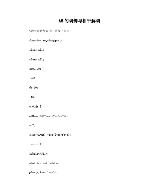
AM的调制与相干解调%四个函数放在同一路径下即可function am_xianggan()close all;clear all;dt=0.001;fm=1;fc=10;T=5;t=0:dt:T;mt=sqrt(2)*cos(2*pi*fm*t);A=2;s_am=(A+mt).*cos(2*pi*fc*t);figure(1);subplot(311);plot(t,s_am);hold on;plot(t,A+mt,'r--');title('AMμ÷??D?o??°??°ü??');xlabel('t');rt=s_am.*cos(2*pi*fc*t);rt=rt-mean(rt);[f,rf]=T2F(t,rt);[t,rt]=lpf(f,rf,2*fm);subplot(312);plot(t,rt);hold on;plot(t,mt/2,'r--');title('?à?é?aμ÷oóD?o?2¨D?ó?ê?è?D?o?μ?±è??'); xlabel('t');subplot(313);[f,sf]=T2F(t,s_am);psf=(abs(sf).^2)/T;plot(f,psf);axis([-2*fc 2*fc 0 max(psf)]);title('AMD?o?1|?ê?×');xlabel('f');function [t st]=F2T(f,sf)%This function calculate the time signal using ifft function for the input %signal's spectrumdf = f(2)-f(1);Fmx = ( f(end)-f(1) +df);dt = 1/Fmx;N = length(sf);T = dt*N;%t=-T/2:dt:T/2-dt;t = 0:dt:T-dt;sff = fftshift(sf);st = Fmx*ifft(sff);function [f,sf]= T2F(t,st)%This is a function using the FFT function to calculate a signal's Fourier %Translation%Input is the time and the signal vectors,the length of time must greater %than 2%Output is the frequency and the signal spectrum dt = t(2)-t(1);T=t(end);df = 1/T;N = length(st);f=-N/2*df:df:N/2*df-df;sf = fft(st);sf = T/N*fftshift(sf);function [ t,st] = lpf( f,sf,B)df=f(2)-f(1);T=1/df;hf=zeros(1,length(f));bf=[-floor(B/df):floor(B/df)]+floor(length(f)/2); hf(bf)=1;yf=hf.*sf;[t,st]=F2T(f,yf);st=real(st);end运行>> am_xianggan()。
am调制matlab代码
am调制matlab代码以下是一份关于AM调制的MATLAB代码,以及对该代码的详细解释。
首先,我们需要明确AM调制的基本原理。
AM调制是一种将信号转换为通过调制一个高频载波信号来传输的技术。
AM调制的基本过程包括将载波信号的振幅按照基带信号的变化进行调制,并通过解调过程将频率重新还原为原始信号。
在MATLAB中实现AM调制的首要任务是生成高频载波信号。
我们可以通过使用sin函数来生成一个正弦波,然后通过调整振幅和频率来创建一个高频信号。
以下是一个生成高频载波信号的MATLAB代码示例:设置参数fc = 1000; 载波频率amplitude = 1; 载波振幅samplingRate = 10000; 采样率time = 1; 生成的信号时间长度生成时间序列t = 0:1/samplingRate:time-1/samplingRate;生成载波信号carrierSignal = amplitude*sin(2*pi*fc*t);在上述代码中,我们定义了载波的频率为1000Hz,振幅为1,并设置了采样率为10000Hz,生成了一个持续1秒的时间序列。
通过将时间序列与正弦函数相乘,我们可以生成一个高频载波信号。
生成的载波信号存储在名为`carrierSignal`的向量中。
接下来,我们需要准备一个基带信号。
基带信号可以是一段音频,也可以是一个控制信号。
在这个例子中,我们将使用一个简单的正弦波作为基带信号。
以下是一个生成基带信号的MATLAB代码示例:设置参数fm = 20; 基带信号频率amplitude = 1; 基带信号振幅生成基带信号basebandSignal = amplitude*sin(2*pi*fm*t);在上述代码中,我们定义了基带信号的频率为20Hz,振幅为1。
通过使用相同的时间序列`t`,我们可以生成一个基带信号。
生成的基带信号存储在名为`basebandSignal`的向量中。
基于MATLAB的AM信号的调制与解调
基于MATLAB的AM信号的调制与解调(陕西理工学院物理与电信工程学院通信工程专业1203班,陕西汉中723003)指导教师:井敏英[摘要]:本文主要的研究内容是了解AM信号的数学模型及调制方式以及其解调的方法。
不同的解调方法在不同的信噪比情况下的解调结果,那种方法更好,作出比较。
进行AM信号的调制与解调。
先从AM的调制研究,研究它的功能及在现实生活中的运用。
其次研究AM的解调,以及一些有关的知识点,以及通过它在通信方面的运用更加深入的了解它。
从AM信号的数学模型及调制解调方式出发,得出AM调制与解调的框图和调制解调波形。
利用MA TLAB编程语言实现对AM 信号的调制与解调,给出不同信噪比情况下的解调结果对比。
[关键词]:AM信号;调制;解调;信噪比MATLAB.Modulation and demodulation of AM signalbased on MATLAB(Grade 2012,Class 3,Major of Communication Engineering,School of Physics and Telecommunication Engineering of Shaanxi University of Technology,Hanzhong 723000,Shaanxi)Tutor: Jing Mingying[Abstract]: The main content of this paper is to understand the mathematical model of the AM signal and the modulation and the demodulation method. Demodulation different methods in different circumstances of the demodulation signal to noise ratio the results of methods that better, to make the comparison. Requirement is more than double the sound and the AM signal modulation and demodulation. AM modulation first study of its function and in real life use. AM demodulation followed by research, as well as some related knowledge, as well as through its use of communications more in-depth understanding of it. AM signal from the tone of the mathematical model and the modulation and demodulation methods,the two-tone AM signal to draw a mathematical model and the block diagram of modulation and demodulation and modulation and demodulation waveforms. MATLAB programming language to use to achieve the two-tone AM signal modulation and demodulation, given the different circumstances of the demodulation signal to noise ratio compared the results.[Keywords]: AM signal, Modulation, Demodulation, Noise ratio signal, MATLAB目录1.绪论背景以及意义现在的社会越来越发达,科学技术不断的在更新,在信号和模拟通信的中心问题是要把载有消息的信号经系统加工处理后,送入信道进行传送,从而实现消息的相互传递。
基于MATLAB的AM信号的调制与解调

基于MATLAB的AM信号的调制与解调(陕西理工学院物理与电信工程学院通信工程专业1203班,陕西汉中723003)指导教师:井敏英[摘要]:本文主要的研究内容是了解AM信号的数学模型及调制方式以及其解调的方法。
不同的解调方法在不同的信噪比情况下的解调结果,那种方法更好,作出比较。
进行AM信号的调制与解调。
先从AM的调制研究,研究它的功能及在现实生活中的运用。
其次研究AM的解调,以及一些有关的知识点,以及通过它在通信方面的运用更加深入的了解它。
从AM信号的数学模型及调制解调方式出发,得出AM调制与解调的框图和调制解调波形。
利用MA TLAB编程语言实现对AM 信号的调制与解调,给出不同信噪比情况下的解调结果对比。
[关键词]:AM信号;调制;解调;信噪比MATLAB.Modulation and demodulation of AM signalbased on MATLAB(Grade 2012,Class 3,Major of Communication Engineering,School of Physics and Telecommunication Engineering of Shaanxi University of Technology,Hanzhong 723000,Shaanxi)Tutor: Jing Mingying[Abstract]: The main content of this paper is to understand the mathematical model of the AM signal and the modulation and the demodulation method. Demodulation different methods in different circumstances of the demodulation signal to noise ratio the results of methods that better, to make the comparison. Requirement is more than double the sound and the AM signal modulation and demodulation. AM modulation first study of its function and in real life use. AM demodulation followed by research, as well as some related knowledge, as well as through its use of communications more in-depth understanding of it. AM signal from the tone of the mathematical model and the modulation and demodulation methods, the two-tone AM signal to draw a mathematical model and the block diagram of modulation and demodulation and modulation and demodulation waveforms. MATLAB programming language to use to achieve the two-tone AM signal modulation and demodulation, given the different circumstances of the demodulation signal to noise ratio compared the results.[Keywords]: AM signal, Modulation, Demodulation, Noise ratio signal, MATLAB目录1.绪论 (1)1.1 背景以及意义 (1)1.2 发展前景 (1)2. AM信号调制原理以及特点 (3)2.1 噪声模型 (3)2.1.1 噪声的分类 (3)2.1.2 本文噪声模型 (3)2.2 通用调制模型 (4)2.3 AM信号的调制原理 (4)2.3.1 AM信号数字模型以及特点 (4)2.3.2 AM信号的波形和频谱特性 (5)3. AM信号的解调原理以及特点 (6)3.1 AM信号的解调原理及方式 (6)3.2 AM信号的相干解调 (6)3.3 AM信号的非相干解调 (6)4. 抗噪声性能的分析模型 (7)4.1 相干解调的抗噪声性能 (7)4.2非相干解调的抗噪声性能 (9)4.3小信噪比情况 (9)5. AM调制与解调的仿真 (9)5.1 AM调制 (9)5.1.1 建立仿真模型 (9)5.1.2 参数设置 (10)5.1.3 仿真波形图 (12)5.2 AM信号的解调仿真 (13)5.2 .1AM相干解调模型仿真 (13)5.2.2参数设置 (13)5.2.3 仿真波形图 (14)5.2.4相干解调抗噪声性能分析 (15)6.AM信号的频谱分析 (16)7.总结 (20)致谢 (21)参考文献 (22)1.绪论1.1 背景以及意义现在的社会越来越发达,科学技术不断的在更新,在信号和模拟通信的中心问题是要把载有消息的信号经系统加工处理后,送入信道进行传送,从而实现消息的相互传递。
《通信原理》课程设计-基于MATLAB的AM信号的调制与解调

课程设计报告院(部、中心)姓名学号专业通信工程班级同组人员课程名称《通信原理》课程设计设计题目名称常规AM方法调制起止时间——2011.6.17成绩指导教师签名基于MATLAB的AM信号的调制与解调摘要:现在的社会越来越发达,科学技术不断的在更新,在信号和模拟电路里面经常要用到调制与解调,而AM的调制与解调是最基本的,也是经常用到的。
用AM调制与解调可以在电路里面实现很多功能,制造出很多有用又实惠的电子产品,为我们的生活带来便利。
在我们日常生活中用的收音机也是采用了AM调制方式,而且在军事和民用领域都有十分重要的研究课题。
本文主要的研究内容是了解AM信号的数学模型及调制方式以及其解调的方法。
不同的解调方法在不同的信噪比情况下的解调结果,那种方法更好,作出比较。
要求是进行双音及以上的AM信号的调制与解调。
先从AM的调制研究,研究它的功能及在现实生活中的运用。
其次研究AM的解调,以及一些有关的知识点,以及通过它在通信方面的运用更加深入的了解它。
从单音AM信号的数学模型及调制解调方式出发,得出双音AM信号的数学模型及其调制与解调的框图和调制解调波形。
利用MA TLAB编程语言实现对双音AM信号的调制与解调,给出不同信噪比情况下的解调结果对比。
关键词:AM信号,调制,解调,信噪比,MATLABModulation and demodulation of AM signalbased on MATLABAbstract: Society becomes more developed now, science and technology in the update, in which signal and analog circuits often used in modulation and demodulation, and AM modulation and demodulation is the most basic, is also frequently used. To participate in the identification of such artificial methods, the ruling includes subjective factors, will vary from person to person, can identify the type of modulation is very limited. Automatic modulation recognition technology can be overcome not only to participate in recognition of artificial difficulties, and the center frequency and bandwidth of the estimation error, adjacent channel crosstalk, noise and interference factors such as the decline of effect is relatively robust. Using AM modulation and demodulation circuit which can achieve a lot of features, creating a lot of useful and affordable electronic products, in order to facilitate our lives. Used in our daily lives is the use of AM radio modulation, but also in the field of military and civilian research topics are very important.The main content of this paper is to understand the mathematical model of the AM signal and the modulation and the demodulation method. Demodulation different methods in different circumstances of the demodulation signal to noise ratio the results of methods that better, to make the comparison. Requirement is more than double the sound and the AM signal modulation and demodulation. AM modulation first study of its function and in real life use. AM demodulation followed by research, as well as some related knowledge, as well as through its use of communications more in-depth understanding of it. AM signal from the tone of the mathematical model and the modulation and demodulation methods, the two-tone AM signal to draw a mathematical model and the block diagram of modulation and demodulation and modulation and demodulation waveforms. MATLAB programming language to use to achieve the two-tone AM signal modulation and demodulation, given the different circumstances of the demodulation signal to noise ratio compared the results.Keyword: AM signal, Modulation, Demodulation, Noise ratio signal, MATLAB一. 课题要求1.1 课程题目已知消息信号m(t)定义为:00010()23230tt t m t t t t ≤<⎧⎪=-≤<⎨⎪⎩其余 用常规AM 方法调制载波, ()cos(2)c c t f t π=,假设f c =250Hz ,t 0=0.15s ,调制指数0.85α=,(1) 导出已调信号的表达式。
基于MATLAB的AM信号的调制
基于MATLAB的AM信号的调制摘要:调制在通信系统中有十分重要的作用。
通过调制,不仅可以进行频谱搬移,把调制信号的频谱搬移到所希望的位置上,从而将调制信号转换成适合于传播的已调信号,而且它对系统的传输有效性和传输的可靠性有着很大的影响,调制方式往往决定了一个通信系统的性能。
MATLAB软件广泛用于数字信号分析,系统识别,时序分析与建模,神经网络、动态仿真等方面有着广泛的应用。
本课题利用MATLAB软件对DSB调制解调系统进行模拟仿真,分别利用300HZ正弦波和矩形波,对30KHZ正弦波进行调制,观察调制信号、已调信号和解调信号的波形和频谱分布,并在解调时引入高斯白噪声,对解调前后信号进行信噪比的对比分析,估计DSB调制解调系统的性能。
关键词:AM信号,调制,调制系数,功率,MATLAB引言:调制就是使一个信号(如光、高频电磁振荡等)的某些参数(如振幅、频率等)按照另一个欲传输的信号(如声音、图像等)的特点变化的过程。
用所要传播的语言或音乐信号去改变高频振荡的幅度,使高频振荡的幅度随语言或音乐信号的变化而变化,这个控制过程就称为调制。
其中语言或音乐信号叫做调制信号,调制后的载波就载有调制信号所包含的信息,称为已调波[1]。
解调是调制的逆过程,它的作用是从已调波信号中取出原来的调制信号。
对于幅度调制来说,解调是从它的幅度变化提取调制信号的过程。
对于频率调制来说,解调是从它的频率变化提取调制信号的过程。
频率解调要比幅度解调复杂,用普通检波电路是无法解调出调制信号的,必须采用频率检波方式,如各类鉴频器电路。
关于鉴频器电路可参阅有关资料,这里不再细述。
随着电脑的发展和普及,调制与解调在电脑通信中也有着十分重要的作用。
通过称为Modem 的调制解调器,将电脑的数字信息转换成能沿着电话线传递的模拟形式,在接收端由Modem 将它转换回数字信息。
其中将数字信息转换成模拟形式称调制,将模拟形式转换回数字信息称为解调。
AM调制解调及matlab仿真程序和图

(1所用滤波器函数:巴特沃斯滤波器% 注 : wp(或 Wp 为通带截止频率 ws(或 Ws 为阻带截止频率 Rp为通带衰减 As 为阻带衰减%butterworth低通滤波器原型设计函数要求 Ws>Wp>0 As>Rp>0function [b,a]=afd_butt(Wp,Ws,Rp,AsN=ceil((log10((10^(Rp/10-1/(10^(As/10-1/(2*log10(Wp/Ws;%上条语句为求滤波器阶数 N为整数%ceil 朝正无穷大方向取整fprintf('\n Butterworth Filter Order=%2.0f\n',NOmegaC=Wp/((10^(Rp/10-1^(1/(2*N %求对应于 N 的 3db 截止频率[b,a]=u_buttap(N,OmegaC;(2傅里叶变换函数function [Xk]=dft(xn,Nn=[0:1:N-1];k=[0:1:N-1];WN=exp(-j*2*pi/N;nk=n'*k;WNnk=WN.^(nk;Xk=xn*WNnk;设计部分:1. 普通 AM 调制与解调%单音普通调幅波调制 y=amod(x,t,fs,t0,fc,Vm0,ma要求 fs>2fc%x调制信号, t 调制信号自变量 ,t0采样区间, fs 采样频率,%fc载波频率, Vm0输出载波电压振幅, ma 调幅度t0=0.1;fs=12000;fc=1000;Vm0=2.5;ma=0.25;n=-t0/2:1/fs:t0/2;x=4*cos(150*pi*n; %调制信号y2=Vm0*cos(2*pi*fc*n; %载波信号 figure(1subplot(2,1,1;plot(n,y2;axis([-0.01,0.01,-5,5];title('载波信号 ';N=length(x;Y2=fft(y2; subplot(2,1,2;plot(n,Y2;title('载波信号频谱 '; %画出频谱波形 y=Vm0*(1+ma*x/Vm0.*cos(2*pi*fc*n; figure(2subplot(2,1,1;plot(n,xtitle('调制信号 ';subplot(2,1,2plot(n,ytitle('已调波信号 ';X=fft(x;Y=fft(y;w=0:2*pi/(N-1:2*pi; figure(3subplot(2,1,1;plot(w,abs(X axis([0,pi/4,0,2000]; title('调制信号频谱 ';subplot(2,1,2;plot(w,abs(Y axis([pi/6,pi/4,0,1200];title('已调波信号频谱 '; %画出频谱波形 y1=y-2*cos(800*pi*n;y2=Vm0*y1.*cos(2*pi*fc*n; %将已调幅波信号的频谱搬移到原调制信号频谱处 wp=40/N*pi;ws=60/N*pi;Rp=1;As=15;T=1; %滤波器参数设计OmegaP=wp/T;OmegaS=ws/T;[cs,ds]=afd_butt(OmegaP,OmegaS,Rp,As; [b,a]=imp_invr(cs,ds,T; y=filter(b,a,y2; figure(4subplot(2,1,1;plot(n,y title('解调波 '; Y=fft(y;subplot(2,1,2;plot(w,abs(Y axis([0,pi/6,0,1000];title('解调信号频谱 '; %画出频谱波形结果:Butterworth Filter Order= 6 OmegaC = 0.1171载波信号载波信号频谱-4-2024调制信号-4-2024已调波信号调制信号频谱已调波信号频谱解调波解调信号频谱解调波解调信号频谱2. 抑制双边带调制与解调%单音抑制载波双边带调制 y=amod(x,t,fs,t0,fc,Vm0,ma要求 fs>2fc %x调制信号, t0采样区间, fs 采样频率,%fc载波频率, Vm0输出载波电压振幅, ma 调幅度t0=0.1;fs=12000;fc=1000;Vm0=2.5;ma=0.25;n=-t0/2:1/fs:t0/2;x=4*cos(150*pi*n; %调制信号y=Vm0*x.*cos(2*pi*fc*n; %载波信号 figure(1subplot(2,1,1plot(n,xtitle('调制信号 ';subplot(2,1,2plot(n,ytitle('已调波信号 ';N=length(x;X=fft(x;Y=fft(y;w=0:2*pi/(N-1:2*pi;figure(2subplot(2,1,1plot(w,abs(Xaxis([0,pi/4,0,2000];title('调制信号频谱 '; %画出频谱波形 subplot(2,1,2plot(w,abs(Y axis([pi/6,pi/4,0,2200];title('已调波信号频谱 '; %画出频谱波形 y1=y-2*cos(2000*pi*n;y2=Vm0*y1.*cos(2*pi*fc*n; %将已调幅波信号的频谱搬移到原调制信号频谱处 wp=40/N*pi;ws=60/N*pi;Rp=1;As=15;T=1; %滤波器参数设计OmegaP=wp/T;OmegaS=ws/T;[cs,ds]=afd_butt(OmegaP,OmegaS,Rp,As; [b,a]=imp_invr(cs,ds,T;y=filter(b,a,y2;figure(3subplot(2,1,1plot(n,ytitle('解调波 ';Y=fft(y;subplot(2,1,2plot(w,abs(Yaxis([0,pi/6,0,5000];title('解调信号频谱 '; %画出频谱波形结果:Butterworth Filter Order= 6 OmegaC = 0.1171调制信号已调波信号500100015002000调制信号频谱500100015002000已调波信号频谱解调波解调信号频谱3. 单边带调制与解调%单音单边带调制 y=amod(x,t,fs,t0,fc,Vm0,ma要求 fs>2fc %x调制信号, t0采样区间, fs 采样频率, %fc载波频率, Vm0输出载波电压振幅, ma 调幅度t0=0.1;fs=12000; fc=1000;Vm0=2.5;ma=0.25; n=-t0/2:1/fs:t0/2; N=length(n;x1=4*cos(150*pi*n; %调制信号 x2=hilbert(x1,N;y=(Vm0*x1.*cos(2*pi*fc*n-Vm0*x2.*sin(2*pi*fc*n/2; figure(1 subplot(2,1,1plot(n,x1 title('调制信号 '; subplot(2,1,2 plot(n,ytitle('已调波信号 '; X=fft(x1; Y=fft(y;w=0:2*pi/(N-1:2*pi; figure(2 subplot(2,1,1plot(w,abs(X axis([0,pi/4,0,3000]; title('调制信号频谱'; subplot(2,1,2 plot(w,abs(Y axis([pi/6,pi/4,0,2500]; title('已调波信号频谱'; %画出频谱波形 y1=y-2*cos(1500*pi*n; y2=Vm0*y1.*cos(2*pi*fc*n; % 将已调幅波信号的频谱搬移到原调制信号频谱处wp=40/N*pi;ws=60/N*pi;Rp=1;As=15;T=1; %滤波器参数设计OmegaP=wp/T;OmegaS=ws/T; [cs,ds]=afd_butt(OmegaP,OmegaS,Rp,As;[b,a]=imp_invr(cs,ds,T; y=filter(b,a,y2; figure(3 subplot(2,1,1 plot(n,y title('解调波';Y=fft(y; subplot(2,1,2 plot(w,abs(Y axis([0,pi/6,0,2500]; title('解调信号频谱'; OmegaC = 0.1171 %画出频谱波形结果:Butterworth Filter Order= 6 %画出频谱波形调制信号 4 2 0 -2 -4 -0.05 -0.04 -0.03 -0.02 -0.01 0 0.01 0.02 0.03 0.04 0.05 已调波信号 10 5 0 -5 -10 -0.05 -0.04 -0.03 -0.02 -0.01 0 0.01 0.02 0.03 0.04 0.05 调制信号频谱 3000 2000 1000 0 0 0.1 0.2 0.3 0.4 0.5 0.6 0.7 已调波信号频谱 2500 2000 1500 1000 500 0 0.55 0.6 0.65 0.7 0.75 解调波 10 5 0 -5 -10 -0.05 -0.04 -0.03 -0.02 -0.01 0 0.01 0.02 0.03 0.04 0.05 解调信号频谱 2500 2000 1500 1000 500 0 0 0.05 0.1 0.15 0.2 0.25 0.3 0.35 0.4 0.45 0.5 7 参考文献 [1] 信号与系统课程组. 信号与系统课程设计指导,2007.10 [2] 吴大正. 信号与线性系统分析(第四版). 高等教育出版社,2005.8[3] 谢嘉奎. 电子线路—非线性部分(第四版. 高等教育出版社,2003,2 [4] 黄永安等.Matlab7.0/Simulink6.0 建模仿真开发与高级工程应用. 清华大学出版社,2005.12 [5] 江建军. LabVIEW 程序设计教程. 电子工业出版社, 2008.03 [6]张化光,孙秋野.MATLAB/Simulink 实用教程. 北京人民邮电出版社, 2009。
- 1、下载文档前请自行甄别文档内容的完整性,平台不提供额外的编辑、内容补充、找答案等附加服务。
- 2、"仅部分预览"的文档,不可在线预览部分如存在完整性等问题,可反馈申请退款(可完整预览的文档不适用该条件!)。
- 3、如文档侵犯您的权益,请联系客服反馈,我们会尽快为您处理(人工客服工作时间:9:00-18:30)。
2、已知消息信号m(t)定义为:
000103()2
230
t
t t m t t t t ≤<⎧⎪
=-≤<⎨⎪⎩其余 用常规AM 方法调制载波, ()cos(2)c c t f t π=,假设f c =250Hz ,t 0=0.15s ,调制指数0.85α=,
(1) 导出已调信号的表达式。
(2) 求消息信号和已调信号的频谱。
(3) 如果该消息信号是周期的,周期为t 0,求在已调信号中的功率和调制效率。
(4) 如果一个噪声信号加到该消息信号上,使解调器输出端的SNR 是10dB ,求该噪声信号的功率。
主程序
am.m echo on
df=0.2; %频率分辨率 A=1;
t0=0.15; %定义t0信号的持续时间的值 ts=0.001; %定义抽样时间 fs=1/ts; %
fc=250; %定义载波频率
snr=10; %定义信噪比,用dB 表示
snr_lin=10^(snr/10); %信噪比的数值 a=0.85; %定义调制系数 t=[0:ts:t0]; %定义出抽样点数 %定义m 信号
%m=[ones(1,ceil(t0/(3*ts))),-2*ones(1,ceil(t0/(3*ts))),zeros(1,ceil(t0/(3*ts)+1))];
m=[1*ones(1,t0/(3*ts)),-2*ones(1,(t0)/(3*ts)),zeros(1,t0/(3*ts)+1)]; c=cos(2*pi*fc.*t); %载波信号 m_n=m/max(abs(m)); u=(1+am_n).*c;
[M,m,df1]=fftseq(m,ts,df); %傅里叶变换,fftseq 函数的程序段见后 M=M/fs; %频率缩放,便于作图 f=[0:df1:df1*(length(m)-1)]-fs/2;%定义频率矢量
%u=(1+a*m_n).*c; %将调制信号调制在载波上 %u=(A*(1+m)).*c;
%u=(A*(1+m)).*c;
[U,u,df1]=fftseq(u,ts,df); %对已调信号作傅里叶变换 U=U/fs; %频率缩放
signal_power=spower(u(1:length(t))); %计算信号的功率,函数spower程序见后%pmn=spower(m(1:length(t)))/(max(abs(m)))^2;%计算调制信号的功率
pmn=(1/4)*spower(m(1:length(t)));
eta=(a^2*pmn)/(1+a^2*pmn); %计算调制效率
noise_power=eta*signal_power/snr_lin; %计算噪声功率
noise_std=sqrt(noise_power); %噪声标准差
noise=noise_std*randn(1,length(u)); %产生高斯分布的噪声
r=u+noise; %总接收信号
[R,r,df1]=fftseq(r,ts,df); %对总信号进行傅里叶变换
R=R/fs; %频率缩放
%以下为结果显示
pause %pause使程序暂停,用户按任意键后继续执行signal_power %显示信号功率
pause
eta %显示调制效率
pause
subplot(2,2,1)
plot(t,m(1:length(t))) %做出调制信号的曲线
axis([0 0.2 -2.1 2.1]);
xlabel('Time')
title('调制信号的曲线');
pause
subplot(2,2,2)
plot(t,u(1:length(t))) %作出已调制信号的曲线
axis([0 0.15 -2.1 2.1]);
xlabel('Time')
title('已调制信号的曲线');
pause
subplot(2,2,3)
plot(t,c(1:length(t))) %作出载波的曲线
axis([0 0.15 -2.1 2.1]);
xlabel('Time')
title('载波的曲线');
pause
subplot(2,1,1)
plot(f,abs(fftshift(M))) %作出频域的调制信号
xlabel('Frequency');
title('频域的调制信号')
pause
subplot(2,1,2)
plot(f,abs(fftshift(U))) %作出频域的已调制信号
title('频域的已调制信号');
xlabel('Frequency')
pause
subplot(2,1,1)
plot(t,noise(1:length(t))) %作出噪声曲线
title('噪声曲线');
xlabel('Time')
pause
subplot(2,1,2)
plot(t,r(1:length(t))) %作出总信号的时域曲线
title('总信号的时域曲线');
xlabel('Time')
pause
subplot(2,1,2)
plot(f,abs(fftshift(R))) %作出频域的总信号曲线
title('频域的总信号曲线');
xlabel('Frequency') ;
程序代码
fftseq.m
function [M,m,df]=fftseq(m,tz,df)
fs=1/ts;
if nargin==2 %判断输入参数的个数是否符合要求
n1=0;
else n1=fz/df; %根据参数个数决定是否使用频率缩放end
n2=length(m);
n=2^(max(nextpow2(n1),nextpow2(n2)));
M=fft(m,n); %进行离散傅里叶变换
m=[m,zeros(1,n-n2)];
df=fs/n;
spower.m
function p=spower(x)
% p=spower(x)
%SPOWER returns the power in signal x
p=(norm(x)^2)/length(x);
0.05
0.1
0.15
0.2
-2
-1
1未调制信号
0.05
0.1
0.15
0.2
-2-1
1
2已调制信号
-500
500
00.050.10.15
0.2未调制信号频谱
-500
500
00.02
0.040.06
0.08已调制信号频谱
0.02
0.04
0.06
0.080.10.12
0.14
0.16
噪声曲线
Time
0.02
0.04
0.06
0.080.1
0.12
0.14
0.16
总信号的时域曲线
Time
00.020.040.060.080.10.120.140.16
-1
Ti m e -500-400-300-200-1000100200300400500
0.00.0.10.频域的总信号曲线
Fr e quency。