Chapt.2 (Model of 1DOF System)
《分布式系统原理与范型:第2版》原书课件第2章

Figure 2-4. The simplified organization of an Internet search engine into three different layers.
•Tanenbaum & Van Steen, Distributed Systems: Principles and Paradigms, 2e, (c) 2007 Prentice-Hall, Inc. All rights reserved. 0-13-239227-5
Structured Peer-to-Peer Architectures (2)
Figure 2-8. (a) The mapping of data items onto nodes in CAN.
•Tanenbaum & Van Steen, Distributed Systems: Principles and Paradigms, 2e, (c) 2007 Prentice-Hall, Inc. All rights reserved. 0-13-239227-5
Multitiered Architectures (1)
The simplest organization is to have only two types of machines:
• A client machine containing only the programs implementing (part of) the userinterface level
Figure 2-9. (a) The steps taken by the active thread.
约翰.金登的多源流分析模型
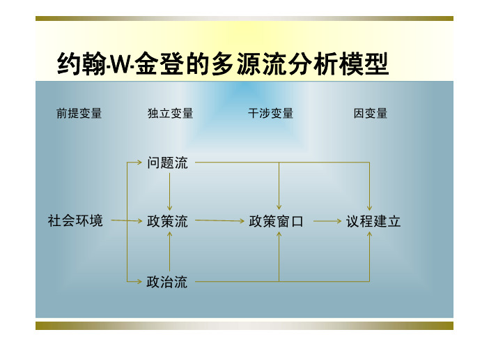
约翰·W·金登的多源流分析模型前提变量独立变量干涉变量因变量问题流社会环境政策流政策窗口议程建立政治流多源流理论在借鉴科恩、马奇、奥尔森的垃圾桶模型的基础上,美国著名的公共政策学家金登建立了多源流理论。
金登认为,“一个项目被提上议程是由于在特定时刻汇合在一起的多种因素共同作用的结果,而并非它们中的一种或另外一种因素单独作用的结果”这种共同作用也就是多源流理论所讲的另外种因素单独作用的结果。
这种共同作用也就是多源流理论所讲的问题流、政策流和政治流三者的连接与交汇。
问题流:由社会环境中的各种社会问题形成的。
各种社会问题在四处漂浮,并不是每一个问题都会被提上政策议程,如何引起决策者的注意取决于某个问题本身的特点。
政策流:在政策原汤中漂浮的各种思想,有的是对未来的模糊概念,有的是专门设计的政策建议。
思想之间相互作用,只有符合某种标准的才能持思想才能坚持下来。
政治流:包括国民情绪、公众舆论、权力分配格局、利益集团实力对比等因素,这些因素反映着政治形势与政治背景等方面的情况。
对于议程状态有明显的促进作用或者抑制作用。
问题流、政策流和政治流之间是彼此独立的,它们的发生、发展和运作都不依赖于其他的源流,但都对政策议程的建立起到促其他的源流但都对政策议程的建立起到促进或者约束的作用。
在某个关键的时间点上,它们汇合到一起,公共问题就会被提上议程,它们汇合到起公共问题就会被提上议程这个关键的时间点就是所谓的“政策之窗”。
政策之窗的含义:是指政策建议的倡导者提出其最得意的解决办法的机会,或者是促使其特殊问题受到关注的机会解决办法的机会,或者是促使其特殊问题受到关注的机会。
政策之窗的类型:(1)以问题为基础的,也被称为“问题之窗”;(2)以政治为基础的,也被称为“政治之窗”。
政策之窗的打开:(1)问题之窗的打开是由于问题流内发生了变化,这种变化的原因大体上又有三种:1)受到广泛关注的指标发生了变化,比如居民消费价格指数(CPI )的猛指标发生了变化比如居民消费价格指数(C增、土地沙漠化面积的扩大、生产安全事件的频发等。
Chapt.6 (2 DOF System)
If desired, can be expressed by θ1 Qθ 2 = θ1 / N Pukyong National University Intelligent Mechanics Lab.
Models of 2-DOF Systems
Free Response
Algebra required closed-form expression for free response of 2-DOF system is more tedious than for 1-DOF system Then, carefully consider whether or not you need a closed-form expression In many applications, only a plot of response is needed If need closed-form, can be used to obtain a plot using numerical method Linear model of 2-DOF system has 4 characteristic roots Free response consists of linear combination of 4 terms, each term corresponding to one root If a root is complex, its solution form expresses as a sine and cosine or a sine function with a phase shift 4 undetermined constants in free response form, require 4 conditions (initial conditions) to evaluate these constants
《chap存储论》PPT课件

• 存储论 (Inventory Theory)
生产和消费是关系国计民生的两件大事,存储 是其间的一个重要环节。即生产→存储→消费。
存储是解决供求间不协调的矛盾的一种手段, 其必要性是显然的。
“存储得越多越好”的思想,不是绝对的。存 储过程中要有一定的损失和消耗,经济上要付出 代价。
C
模型一:不允许缺货,一次性补充
t* 2C3 C1R
Q* Rt* 2C3R C1
C * C * (t) 2C3C1R
第七章 存储论 复习 (Inventory Theory)
确定性存储模型:模型中的数据皆为确定的数值
随机性存储模型: 模型中含有随机变量,而不是确定
的数值
确定性存储模型按入库速率类型和满足需求程度类型, 分为4种类型: 模型一:不允许缺货,一次性补充 模型二:不允许缺货,生产需一定时间 模型三:允许缺货(缺货需补足),生产时间很短 模型四:允许缺货(缺货需补足),生产需一定时间
二、研究原则
存储论是以库存总费用最小的原则来研究存储模型的。
三、存储论的基本概念
1、存储系统: 是一个由补充、存储、需求三个
环节紧密构成的现实运行系统。
补充
存储
需求
输入
订购进货 仓库 供给需求 (库存量)
输出
2、补充(订货和生产):存储量由于需求减
少,必须加以补充,这是存储的输入。
➢批量:每一批补充数量QO ➢补充间隔:两次补充之间的时间t0 ➢提前期(拖后期): 补充存储的时间 提前期:可长,可短, 确定性的, 随机性的
2
3
4
5
概率P(r)
0.05 0.1 0.25 0.35 0.15 0.1
chap2-古典密码

密钥 密文
密钥
明文
加密算法
明文 解密算法
加密密钥(Encryption Key) 解密密钥(Decryption Key)
基本概念
需要密钥的加密算法,记为:C=E(K,P),即密文消息同时
依赖于初始明文和密钥的值。实际上,E是一组加密算法, 而密钥则用于选择其中特定的一个算法。
加密与解密的密钥相同,即:P=D(K,E(K,P)) 加密与解密的密钥不同,则:P=D(K ,E(K ,P))
除了一次一密的方案外,没有无条件安全的算法 安全性体现在任意一条:
• 破译的成本超过加密信息的价值 • 破译的时间超过该信息有用的生命周期
密钥搜索所需平均时间
目录
1.
2. 3.
密码学的起源、发展和现状
密码学基本概念 典型几种古典密码技术
经典加密技术
替代 置换 隐写术
古典密码:替代(代替)
2018/6/26
41/72
古典密码:置换
改变明文内容元素的相对位置,保持内容的表现形式不 变 通常称为transposition或者permutation密码 通过重新安排消息字母的位置来隐藏明文信息,而不是 用其他字母来代换明文字母 这种方法是很容易破译的,因为密文拥有与明文一样的 字母频率统计特性
(4)任意k∈ K,有一个加密算法 ek E 和相应的解密 算法 d k D ,使得 ek : P C 和 dk : C P 分别为加 密解密函数, 满足dk(ek(x))=x ,这里 x ∈P。
密码编码系统分类
保密内容 密钥数量 明文处理的方式
保密内容
受限制的(restricted)算法
chap2

2.2
语
法
函数的归约公理 仅把β公理定向为从左到右的归约规则 η归约用于λ演算的许多版本中 归约用于λ
2.2
语
法
curry算子将多元函数变换成高阶函数 算子将多元函数变换成高阶函数 算子将 Curry = def λf : nat × nat → nat.λx : nat.λy : nat.f x, y λ λ Curry(add) ≡ (λf : nat × nat → nat.λx : nat.λy : nat.f x, y) λ λ λ add = λx : nat. λy : nat.add x, y ≡ λx : nat. λy : nat.(λp : nat × nat.(Proj1 p) + λ (Proj2 p)) x, y = λx : nat. λy : nat. Proj1x, y + Proj2 x, y = λx : nat. λy : nat.x + y
2.2
语
法
2.2.1 概述 由列出PCF的类型来概括其构造 由列出 的类型来概括其构造 基本类型:nat和bool 基本类型: 和 类型构造符
– 笛卡儿积σ×τ – 函数类型σ→τ
规定:→右结合,×的优先级高于→ 规定: 右结合, 的优先级高于→ 高于
– –
σ→τ→ρ等同于σ→(τ→ρ) σ×τ→ρ等同于 σ×τ)→ρ 等同于( →
阶乘函数是方程(f : nat → nat = 阶乘函数是方程( λy : nat.if Eq? y 0 then 1 else y f (y – 1) )的解 的解 阶乘函数是 F =def λf : nat → nat.λy : nat.if Eq? y 0 then 1 λ else y f (y – 1) 的不动点
精算模型第二版课后习题答案(上)
(
.0)6$%
.!000
槡0)6
超出%"!000 槡0)6的部分为%
" !! !!/-"189:0)60!"".
!000 (2(<2 % !000(
.6;).*,;
除以!’-"0)!!我们得到6;.)*,;$ 同样的结果可以通过方程解出%
" # !!&!%""
% !000
(
"-$%"!000槡-
整合可得
+++
"(#C9D9#=>?@A?B分布与对数正态分布’"+#逆指数分布与指数分布$ 解%4=>#=>?@A?B分布只有正数阶矩!而伽玛分布都有!所以 4=>#=>?@A?B分布比伽玛分 布有更厚的尾部$
C9D9#=>?@A?B分布只有正数阶矩!而对数正态分布都有!所以 C9D9#=>?@A?B分布比对数 正态分布有更厚的尾部$
所以!# 的分布是一个参数#"!&!的指数分布$ (!已知%"!#" 服从均值为(的指数分布’"(##""!)*$计算’(#()$ 解%使用#(""+ 的代换来计算指数分布的三阶矩更为简单$
!!’!#(""’!"+""+##+",-(+"./
+!" 服从一个参数为!"()*!#"!0的伽玛分布$#"!&"!计算()*"##$ 解%我们来计算’"##和’"#(#!或者’""’!#和’""’(#!注意到 12345 中用于 伽玛分布整数阶矩计算的公式’""+#"#+"!%+’!#*!$这个公式值提供了当+ 是一个正 整数的情况!所以不能够用来计算’!和’(阶矩$由此!我们必须使用 12345 中更为 一般化的公式
第七章人工神经网络
2003-11-1
高等教育出版社
27
三层前向神经网络
考虑一个三层的前向神经网络,设输入
层层节节点点数数为为nm1。,设中间Yi1为层输节入点层数节为点n2,i的输输出
出;Y
2 j
为中间层节点j的输出;Yk3
为输出
层的权θ点节教值jk为的点师;中阈信kW间的值j号k层为输。;节节出W点点;ij为jjT的和k节为阈节点输值点i出和;k间层节θ的节点k为连点j间输接k的出对权连层应值接节;
y
sgn
Wi Ii
2003-11-1
高等教育出版社
5
人工神经元的形式化描述
人工神经元的数学模型如图所示
x1 x2
… ‥ xn
u育出版社
6
人工神经元的形式化描述(续)
其中ui为第i个神经元的内部状态,θi为神经元 阈值,xj为输入信号,wji表示从第j个神经元到 第i个神经元连接的权值。si表示第i个神经元的 外部输入信号,上述假设可描述为:
ui
f
j
x j wji
si
i
yi gui h
x j wji
si
i
j
hg f
2003-11-1
高等教育出版社
7
常用的神经元状态转移函数
阶跃函数
1 y f (x) 0
x0 x0
准线形函数
1
y f (x) x
0
x 0 x
x0
Sigmoid函数
f
x
1
1 ex
双曲正切函数 f (x)=th (x)
出输入样本的网络预测。有
两个隐层的前向神经网络如
•••
图所示:
伍德里奇《计量经济学导论》复习笔记和课后习题详解-含有定性信息的多元回归分析:二值变量
伍德里奇《计量经济学导论》复习笔记和课后习题详解-含有定性信息的多元回归分析:二值变量第7章含有定性信息的多元回归分析:二值(或虚拟)变量7.1复习笔记考点一:带有虚拟自变量的回归★★★★★1.对定性信息的描述定性信息是指通常以二值信息(0-1)的形式出现的信息,如性别、是否结婚等。
在计量经济学中,二值变量又称为虚拟变量。
2.只有一个虚拟自变量(1)只有一个虚拟自变量的简单模型考虑决定小时工资的简单模型:wage=β0+δ0female+β1educ +u。
根据多元回归的解释方式,δ0表示控制educ不变时,female 变化1单位给wage带来的变化。
假定零条件均值假定E(u|female,educ)=0成立,那么:δ0=E(wage|female=1,educ)-E (wage|female=0,educ),其中female=1表示女性,female =0表示男性。
可以发现,在任意教育水平下,男性与女性的工资差异是固定的,女性工资比男性工资多δ0。
除了β0之外,模型中只需要引入一个虚拟变量。
因为female+male=1,所以引入两个虚拟变量会导致完全多重共线性,即虚拟变量陷阱。
(2)当因变量为log(y)时,对虚拟解释变量系数的解释当变量中有一个或多个虚拟变量,且因变量以对数的形式存在时,虚拟变量的系数可以理解为百分比的变化。
将虚拟变量的系数乘以100,表示的是在保持所有其他因素不变时y 的百分数差异,精确的百分数差异为:100·[exp(∧β1)-1]。
其中∧β1是一个虚拟变量的系数。
3.使用多类别虚拟变量(1)在方程中包括虚拟变量的一般原则如果回归模型具有g 组或g 类不同截距,一种方法是在模型中包含g-1个虚拟变量和一个截距。
基组的截距是模型的总截距,某一组的虚拟变量系数表示该组与基组在截距上的估计差异。
如果在模型中引入g 个虚拟变量和一个截距,将会导致虚拟变量陷阱。
另一种方法是只包括g 个虚拟变量,而没有总截距。
Chapter-2(第三版教材)
Discrete-Time Signals: Time-Domain Representation
• A right-sided sequence x[n] has zerovalued samples for n < N1
A right-sided sequence
•If N1 0, a right-sided sequence is called a causal sequence
In some applications, a discrete-time sequence {x[n]} may be generated by periodically sampling a continuous-time signal xa(t) at uniform intervals of time
Discrete-Time Signals: Time-Domain Representation
• Discrete-time signal may also be written as a sequence of numbers inside braces: {x[n]}={…,-0.2,2.2,1.1,0.2,-3.7,2.9,…} • The arrow is placed under the sample at time index n = 0 • In the above, x[-1]= -0.2, x[0]=2.2, x[1]=1.1, etc.
Discrete-Time Signals: Time-Domain Representation
• Graphical representation of a discrete-time signal with realvalued samples is as shown below:
- 1、下载文档前请自行甄别文档内容的完整性,平台不提供额外的编辑、内容补充、找答案等附加服务。
- 2、"仅部分预览"的文档,不可在线预览部分如存在完整性等问题,可反馈申请退款(可完整预览的文档不适用该条件!)。
- 3、如文档侵犯您的权益,请联系客服反馈,我们会尽快为您处理(人工客服工作时间:9:00-18:30)。
Outline
This chapter introduces the model to derive the correction description of the dynamics of the system with one degree of freedom. The principles can be easily extended to obtain models of systems having two or more degrees of freedom (Chap. 6 and 8). Pukyong National University Intelligent Mechanics Lab.
Note how much simpler the velocity and acceleration expressions are when described by normal-tangential coordinates
Pukyong National University
Intelligent Mechanics Lab.
Pukyong National University
Intelligent Mechanics Lab.
Degree of Freedom
Degree of freedom (DOF) : the minimum number of coordinates required to completely describe the motion of the object Generalized coordinates : coordinates that reflect the existence of constraints and yet still provide a complete description of the motion of the object (For pendulum, angle θ, coordinate x and y are not) Constraint : restrict the motion of an object usually means that fewer coordinates are needed to describe the motion of the object (constant length L)
Curvilinear Translation
Rectilinear Translation
General Plane Motion
Fixed-axis Rot University
Intelligent Mechanics Lab.
Kinematics
Example : Single Pendulum
A system having 1 DOF
A multi-pulley system
Pukyong National University
Intelligent Mechanics Lab.
Plane Motion of a Rigid Body
Particle : A mass of negligible dimensions Motion can consist of translation only Rigid body : An object negligible deformations but considered dimensions Motion can involve both translation and rotation Newton’s second law : Acceleration of a mass particle is proportional to the vector resultant force acting on it and is in the direction of this force
Kinematics
Kinematics (운동학 운동학, 운동학 動 ):
• Study of motion only without regard for the masses that are in motion or the forces that produce the motion • Primarily concerned with relationship among displacement, velocity & acceleration • Provides the basis for describing the motion of the systems • Restrict our attention to motion in a plane • This means that the object can translate in 2-dimensions only and can rotate only about an axis that is perpendicular to the plane containing these 2-dimensions • The completely general motion involves translation in 3-dimensions and rotation about 3-axes : considerably more complex to analyze • Many practical engineering problems can be handled with the plane motion methods
∑ F = f = ma = m dt
dv dv
Vector sum of external forces acting on a body of mass m must equal the time rate of change of linear momentum L
f= d (mv ) dL = dt dt
String or cable
• Infinite DOF • y = f(x)
Pukyong National University
Intelligent Mechanics Lab.
Coordinates & Degree of Freedom
Examples : DOF & Kinematics
• If without constraint 3 translations 3 rotations 6 DOF
• If with constraint (only vertical motion) 1 translations (x) 1 DOF
Pukyong National University
Coordinates
Coordinate : An independent quantity used to specify position The proper choice of coordinates can simplify the resulting expression for position, velocity, or acceleration Categories of coordinates : Fixed or moving rectangular coordinate Path coordinate (normal-tangential coordinate) Polar coordinate (cylindrical coordinate)
• 2 DOF • Generalized coordinates (θ1, θ2)
• 2 DOF • Generalized coordinates (x1, x2)
• Pure rolling motion • 1 DOF (∆x = R∆θ) • Generalized coordinates θ or x
Normal and tangential coordinate system Fixed rectangular coordinate system
Velocy vecor : & v = v e = Lθ e
t
t
Acceleration vector : v2 & && & a = e n + v et = Lθ 2 e n + Lθ et L
Equilibrium
힘( ) (force)
Pukyong National University
물체
운동( 動) (motion)
Intelligent Mechanics Lab.
Kinematics
Kinematics : Categories of Plane Motion
Translation(¿ 動), Rotation(eo 動) 4 categories of plane motion • Rectilinear translation • Curvilinear translation • Rotation about a fixed axis • General plane motion
M=
d ( Iω) dH & = =H dt dt
I : Body’s mass moment of inertia about the axis & ω : Angular velocity about that axis (ω = θ ) Term torque T are often used instead of moment Calculating inertia : mass moment of inertia I about a specified reference axis
William J. Palm III : Mechanical Vibration