Porting a vector library a comparison of mpi, paris, cmmd and pvm
APX 8000H 品牌:Motorola 产品名:通信设备 型号:APX 8000H说明书

360 Degrees of ProtectionWe know the job puts your officers in harm’s way every day. The last thing they need to worry about is safe communication. Certified to the stringent Div1 HazLoc standards, the APX 8000H is designed for use in areas where there are routinelydangerous concentrations of flammable gases, vapors, liquids or combustible dust. No heat. No sparks. No worries.Of course, communication matters too. Your officers can’t afford not to hear—or be heard. The APX 8000H has an adaptive audio engine that provides the loudest, clearest audio at any volume, in any environment. We also know that they need to connect with outside agencies, often without a moment to spare. The APX 8000H transmits and receives on all commonly used frequencies, so they can communicate with different agencies using the same radio. With its intuitive design and comfortable feel, the APX 8000H is made for the way your officers work.APX ™8000HALL-BAND P25 HAZLOCPORTABLE RADIO6.3 i n (160 m m )0.7 i n (19 m m )1.9 i n (49 m m ) 3.0 in (76mm)Weight with standard battery20 oz (568 g)Accessory connector with water / dust sealWaterproof speakerNon-slip PTT buttonMulti-microphoneAvailable with full or limited keypadRecess for custom labeling3x sideprogrammable Angled volume knob Top display for on-belt status updatesINGRESS PROTECTIONIP68 submersion (2m, 2hr)MIL-STD Delta-T, IP86 (2m, 4hr)1OTHER FEATURESText Messaging Voice Announcements Radio Profiles Dynamic Zone Intelligent Lighting IMPRES 2 Battery RFID Volume Knob 1Digital Tone Signaling 1Instant RecallIntelligent Priority ScanHeight (radio body) 6.9 in (176.5 mm)Width 3.3 in (84 mm)Depth2.2 in (56 mm)Weight (Model3.5 & 2.5)22.9 oz (650 g)Weight (Model 1.5)23.4 oz (662 g)SECURITYSingle-key ADP Encryption Software Key P25 Authentication 1Multikey for 128 keys and multi-algorithm 1Over-the-air Rekeying (OTAR)1Features1 Optional.2Review accessory catalog and UL manual for more details. 3Review UL manual for more details.*Groups C only applies to ULOPERATION MODESDigital Trunking: 9600 Baud APCO P25 Phase 1 FDMA and Phase 2 TDMA Analog Trunking: 3600 Baud SmartNet®, SmartZone®, Omnilink Digital Conventional: APCO 25Analog Trunking: MDC 1200, Quik-Call II ASTRO 25 Integrated Voice & DataAUDIO FEATURES3 W Speaker with Adaptive Equalization Adaptive Dual-sided Operation Adaptive Noise Suppression Intensity Adaptive Gain Control Adaptive WindportingCompatible with IMPRES 2 Audio Accessories 2SRX PACKAGE FEATURES**Coyote Brown Color NVG Compability Light Discipline Lens Blacked-out LogoMIL-STD Delta-T, IP68 (2 m, 4 hr)CONNECTIVITYMission-Critical Bluetooth (version 4.0)Wi-Fi (802.11b/g/n)1Data Modem Collaboration over Wi-Fi 1SmartConnect via WiFi 1MANAGEMENTCustomer Programming Software (CPS), version R12.00.00 or later Radio ManagementOver-the-air Programming (OTAP)1SAFETYLocation-Tracking (GPS and GLONASS)Mission-critical Geofence 1Man Down / Fall Alert1MODELS AVAILABLEAll-band: VHF, UHF (ranges 1 and 2), 700 and 800 MHzHAZLOC (UL/CSA)Class I, Div 1, Groups C*, D;Class I, Div 2, Groups A, B, C, D; Class II, Div 1, Group E, F, G;Class III; T3C.3**For critical communications in military applications, such as installation security and force protection, we offer an optional SRX package.Check with your Motorola Solutions representative for SmartConnect availability in your area.RADIO MODELSDisplay Full bitmap color LCD front display• 2 lines of status icons• 4 lines of text x 14 characters• 1 line of menu x 3 keys• White backlightFull bitmap color LCD front display• 2 lines of status icons• 4 lines of text x 14 characters• 1 line of menu x 3 keys• White backlightFull bitmap mono LCD top display• 1 line of text x 8 characters• 1 line of status icons• Multi-color backlightFull bitmap mono LCD top display• 1 line of text x 8 characters• 1 line of status icons• Multi-color backlightKeypad4x3 keypad-3 soft keys 3 soft keys4-way navigation pad4-way navigation pad Home key Home keyData key Data keyChannel Capacity30003000 FLASHport Memory 2 GB 2 GB Part Number H91TGD9PW9AN H91TGD9PW8ANButtons and SwitchesNon-slip PTT button Non-slip PTT buttonEmergency button (orange)Emergency button (orange)Power / volume knob (angled)Power / volume knob (angled)Rotary selector, 16-position Rotary selector, 16-positionConcentric switch, 2-position Concentric switch, 2-positionA/B/C switch, 3-position A/B/C switch, 3-position3 programmable side buttons 3 programmable side buttons Standard StandardSRX Package SRX PackageTRANSMITTERFrequency Range / Bandsplits136-174 MHz380-470 MHz450-520 MHz762-776, 794-806 MHz806-825, 851-870 MHz Channel Spacing112.5 / 20 / 25 kHz12.5 / 20 / 25 kHz12.5 / 20 / 25 kHz12.5 / 20 / 25 kHz12.5 / 20 / 25 kHz Maximum Frequency Separation Full Bandsplit Full Bandsplit Full Bandsplit Full Bandsplit Full Bandsplit Rated RF Output Power (Adjustable)21-6 W1-5 W1-5 W1-2.5 W1-3 W Frequency Stability (-30 °C to +60 °C; +25 °C Ref.)2±1.0 ppm±1.0 ppm± 1.0 ppm± 1.0 ppm± 1.0 ppm Modulation Limiting (12.5 / 20 / 25 kHz channel)2±2.5 / ±4 / ±5 kHz±2.5 / ±4 / ±5 kHz±2.5 / ±4 / ±5 kHz±2.5 / ±4 / ±5 kHz±2.5 / ±4 / ±5 kHz Emissions (conducted and radiated)2-75 dBc-75 dBc-75 dBc-75 dBc-75 dBcAudio Response2+1, -3 dB +1, -3 dB +1, -3 dB +1, -3 dB +1, -3 dBFM Hum and Noise (12.5 / 25 kHz channel)2-51 / -51 dB-51 / -51 dB-47 / -51 dB-47 / -49 dB-46 / -49 dBAudio Distortion (12.5 / 25 kHz channel)20.90% / 0.50%0.90% / 0.50%0.90% / 0.60%0.90% / 0.90%0.90% / 0.60% RECEIVERFrequency Range / Bandsplits136-174 MHz380-470 MHz450-520 MHz762-776MHz851-870 MHz Channel Spacing112.5 / 20 / 25 kHz12.5 / 20 / 25 kHz12.5 / 20 / 25 kHz12.5 / 20 / 25 kHz12.5 / 20 / 25 kHz Maximum Frequency Separation Full Bandsplit Full Bandsplit Full Bandsplit Full Bandsplit Full Bandsplit Audio Output at Rated2 3 W 3 W 3 W 3 W 3 WAudio Output at Max2 5 W 5 W 5 W 5 W 5 WFrequency Stability (-30 °C to +60 °C; +25 °C Ref.)2±1.0 ppm±1.0 ppm±1.0 ppm±1.0 ppm±1.0 ppmAnalog Sensitivity (12 dB SINAD) Standard20.168 µV(-122.5 dBm)0.199 µV(-121.0 dBm)0.199 µV(-121.0 dBm)0.224 µV(-120.0 dBm)0.224 µV(-120.0 dBm)Digital Sensitivity (1% BER)30.251 µV(-119.0 dBm)0.282 µV(-118.0 dBm)0.282 µV(-118.0 dBm)0.316 µV(-117.0 dBm)0.316 µV(-117.0 dBm)Digital Sensitivity (5% BER)30.149 µV(-123.5 dBm)0.158 µV(-123.0 dBm)0.158 µV(-123.0 dBm)0.211 µV(-120.5 dBm)0.211 µV(-120.5 dBm)Selectivity (12.5 / 25 kHz channel)2-77 / -82 dB-74 / -80 dB-74 / -80 dB-72 / -79 dB-72 / -78 dB Intermodulation (12.5 / 25 kHz channel) Standard2-82 dB-80 dB-80 dB-81 dB-80 dBSpurious Rejection2-92 dB-98 dB-98 dB-98 dB-98 dBFM Hum and Noise (12.5 / 25 kHz channel)2-55 / -57 dB-54 / -56 dB-54 / -56 dB-53 / -55 dB-52 / -54 dBAudio Distortion20.90%0.90%0.90%0.90%0.90% BATTERIESPMNN4547Li-Ion IMPRES 23100 mAh Y 3.4 x 2.3 x 1.8 in (86 x 59 x 45 mm)7.1 oz (201 g)Standard1 Please refer to local regulations for available channel bandwidths.2 Measured conductively in analog mode per TIA / EIA 603 under nominal conditions.3 Measured conductively in digital mode per TIA / EIA IS 102.ENCRYPTIONSupported Encryption Algorithms ADP, 256-bit AES, DES, DES-XL, DES-OFB, DVP-XL, Localized AlgorithmEncryption Algorithm Capacity8Encryption Keys per Radio 1024 keysProgrammable for 128 Common Key References (CKR) or 16 Physical Identifiers (PID)Encryption Frame Re-sync Interval360 ms (P25 CAI)Encryption Keying Local Key Loader and Over the Air Rekeying (OTAR)Synchronization XL – Counter Addressing OFB – Output FeedbackVector Generator National Institute of Standards and Technology (NIST) approved random number generatorEncryption Type Digital and SecureNetKey Storage Tamper-protected volatile or non-volatile memory Key Erasure Keyboard command and tamper detectionStandards FIPS 140-3 Level 3FIPS 197OTHER OPTIONSHousing Color OptionsStandard: BlackSRX Package: Coyote BrownGPSConstellations GPS and GLONASS Tracking Sensitivity-164 dBmAccuracy1<5 meters (95%)Cold Start1<60 seconds (95%)Hot Start1<5 seconds (95%)Mode of Operation Autonomous (Non-Assisted)AUDIOAudio Output at Rated 3 WAudio Output at Max 5 WAudio Response (EIA)+1, -3 dBSpeech Loudness at 12 in (300 mm)105 phonAudio FeaturesAdaptive EqualizationAdaptive Dual-sided OperationAdaptive Noise Suppression IntensityAdaptive Gain ControlAdaptive WindportingIMPRES 2 AudioWIRELESSFrequency Range: 2402 - 2480 MHzMission Critical Wireless Bluetooth 2.1 uses 96 bit encryption for pairing and 128 bit encryption forvoice, signaling and data. The radio supports up to 6 data connectionsand 1 audio connectionBluetooth Low Energy uses 128-bit AES-CCM encryptionWi-Fi® 802.11 b/g/nFrequency Range: 2400 - 2483.5 MHzSupports WPA-2, WPA, WEP security protocolsRadio can be pre-provisioned with up to 20 SSIDsREGULATORY INFORMATIONFCC ID All-Band AZ489FT7111IC ID All-Band109U-89FT7111EmissionDesignatorsLMR8K10F1D, 8K10F1E, 8K10F1W, 11K0F3E,16K0F3E, 20K0F1EBluetooth852KF1D, 1M17F1D, 1M19F1DWLAN (Wi-Fi)13M7G1D, 17M0D1D, 18M1D1DENVIRONMENTALOperating Temperature-20 to +60 ºC (-20 to +140 ºF)Storage Temperature1-40 to +85 ºC (-40 to +185 ºF)Humidity Per MIL-STD 810ESD IEC 61000-4-2Dust Resistance IP6XWater Resistance(Submersion) IPX8 (2 meters, 2 hours);Option MIL STD (Delta-T) and IPX8 (2 meters, 4 hours)Leakage (Immersion)MIL-STD-810 C, D, E, F and G1 Radio only. To ensure best performance, batteries should be stored at 25 °C, ±5 °C .2 Submersion tests conducted using more stringent, preheated (Delta-T) method..For more information, please visit:/apxMIL-STDLow Pressure 500.1I 500.2II 500.3II 500.4II 500.5II High Temperature 501.1I,II 501.2I/A1, II/A1501.3I/A1, II/A1501.4I/Hot, II/Hot 501.5I/A1, II/A1Low Temperature 502.1I 502.2I/C3, II/C1502.3I/C3, II/C1502.4I/C3, II/C1502.5I/C3, II/C1Temperature Shock 503.1I 503.2I/A1/C3503.3I/A1/C3503.4I 503.5I-C Solar Radiation 505.1II 505.2I 505.3I 505.4I 505.5I/A1Rain 506.1I,II 506.2I,II 506.3I,II 506.4I,III 506.5I,III Humidity 507.1II 507.2II 507.3II 507.4 1 Proc 507.5II/Aggravated Salt Fog 509.1I 509.2I 509.3I 509.4 1 Proc 509.5 1 Proc Blowing Dust 510.1I 510.2I 510.3I 510.4I 510.5I Explosive Atmosphere --511.2I 511.3I 511.4I 511.5/6I Blowing Sand 1 Proc 1 Proc 510.2II 510.3II 510.4II 510.5II Submersion 2512.1I 512.2I 512.3I 512.4I 512.5I Submersion (Salt Water)2512.1I512.2I512.3I512.4I512.5IVibration 514.2VIII,F , Curve-W514.3I/10, II/3514.4I/10, III/3514.5I/24, II/5514.6I/24, II/5Shock 516.2I, V516.3I, VI516.4I, VI516.5I, VI516.6I, VIShock (Drop)516.2II516.2IV516.4IV516.5IV516.6IVMotorola Solutions, Inc. 500 West Monroe Street, Chicago, IL 60661 U.S.A. MOTOROLA, MOTO, MOTOROLA SOLUTIONS and the Stylized M Logo are trademarks or registered trademarks of Motorola Trademark Holdings, LLC and are used。
实验一 OptiSystem仿真组件库介绍
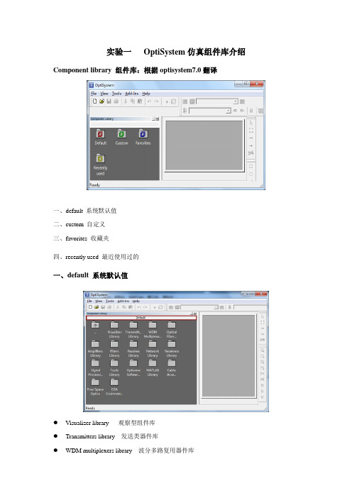
实验一OptiSystem仿真组件库介绍Component library 组件库:根据optisystem7.0翻译一、default 系统默认值二、custom 自定义三、favorites 收藏夹四、recently used 最近使用过的一、default 系统默认值●Visualizer library 观察型组件库●Transmitters library 发送类器件库●WDM multiplexers library 波分多路复用器件库●Optical fibers library 光纤器件库●Amplifiers library 放大器组件库●Filters library 滤波器器件库●Passives library 无源器件库●Network library 网状器件库●Receivers library 接收端器件库●Signal processing library 信号处理器件库●Tools library 工具类器件库●Optiwave software tools 光波类软件库●Matlab library Matlab组件库●Cable access library 有线接收器件库●Free space optics 自由空间光●EDA cosimulation library 电子设计自动化仿真组件库(1)Visualizer library观察型组件库Optical 光学类Test sets:Optical filter analyzer 光学滤波式分析器(测试设备)Photonic all-parameter analyzer 光电子全参量分析器Differential mode delay analyzer 差模延迟分析器Optical spectrum analyzer 光谱仪Optical time domain visualizer 光时域观察仪Optical power meter 光功率计WDM analyzer 波分复用分析仪Dual port WDM analyzer 双端口波分复用分析仪Polarization analyzer 检偏振器Polarization meter 偏振仪表Spatial visualizer 空间立体观察器Encircled flux analyzer 环型通量分析仪Electrical 电学类Test sets:Electrical filter analyzer 电子类滤波器分析S parameter extractor S参量提取器Oscilloscops visualizer 示波器RF spectrum analyzer 射频频谱分析仪Eye diagram analyzer 眼图BER analyzer 误码率分析仪Electrical power meter visualizer 功率表Electrical constellation visualizer 万用表Electrical carrier analyzer 载波分析(2) Transmitters library 发送机组件Optical sources光源CW laser 连续波激光器Laser rate equations 速率方程Laser measured 激光测量LED 发光二极管White light source 白光Pump laser 激光泵浦Pump laser array 激光泵浦阵列CW laser array 连续激光阵列CW laser measured 连续波激光测量Directly modulated laser measured 调制激光直接测量CW laser array ES 连续波激光回声探测VCSEL laser 垂直端面发射激光器Controlled pump laser 可控泵浦激光Spatial CW laser 空间连续波激光器Spatial laser rate equations 空间激光速率方程组Spatial LED 空间发光二级管Spatial VCSEL 空间垂直端面发射激光器Spatiotemporal VCSEL 空域/时域垂直端面发射激光器Bit sequence generators 码元产生器Pseudo-random bit sequence generator 伪随机码发生器User defined bit sequence generator 用户自定义码发生器Pulse generators 脉冲发生器Electrical : RZ pulse generator 归零脉冲发生器NRZ pulse generator 非归零脉冲发生器Gaussian pulse generator 高斯脉冲发生器Hyperbolic-secant pulse generator 双曲正割脉冲发生器Sine generator 正弦波产生器Triangle pulse generator 三角脉冲产生器Saw-up pulse generator 上升锯齿波产生器Saw-down pulse generator 下降锯齿波产生器Impulse generator 脉冲产生器Raised cosine pulse generator 升余弦脉冲Sine pulse generator 正弦脉冲Measured pulse 测量脉冲Measured pulse sequence 测量脉冲组Bias generator 电流偏差产生器Duobinary pulse generator 二进制脉冲产生器Electrical jitter 电抖动Noise source 噪声源Predistortion 预失真、预矫正M-ary pulse generator M进制脉冲发生器M-ary raised cosine pulse generator M进制升余弦脉冲发生器Optical: Optical Gaussian pulse generator 高斯光脉冲产生器Optical sech pulse generator 双曲正割光脉冲产生器Optical impulse generator 光测量脉冲发生器Measured optical pulse 测量脉冲Measured optical pulse sequence 测量光脉冲组TRC measurement date TRC测量数据Spatial optical gaussian pulse generator 高斯空间光脉冲产生器Spatial optical impulse generator 空间光脉冲产生器Spatial optical sech pulse generator 双曲正割空间光脉冲产生器Optical modulators 光调制器Mach-zehnder modulator M-Z调制器Electroabsorption modulator 电吸收调制器Amplitude modulator 调幅Phase modulator 调相Frequency modulator 调频Dual drive Mach-zehnder modulator measured 双驱动M-Z调制器Electroabsorption modulator measured 电吸收调制器Single drive Mach-zehnder modulator measured 单驱动M-Z调制器Dual port dual drive Mach-zehnder modulator measured 双端口双驱动M-Z调制器LiNb Mach-zehnder modulator LiNb M-Z调制器Optical transmitters 光发送机WDM transmitter 波分复用光发送机Spatial optical transmitter 空间光发送机Optical transmitter 光发送机Multimode 多模Multimode generator 多模产生器Laguerre transverse mode generator 拉盖尔横模产生器Donut transverse mode generator 环行横模产生器Measured transverse mode generator 可调横模产生器(3) WDM multiplexers library WDM多路复用器Add and drop 分插复用WDM add 合复用器WDM drop 分复用器WDM add and drop 分插复用器Demultiplexers 解复用器WDM demux 1x2 1x2解复用器WDM demux 1x4 1x4解复用器WDM demux 1x8 1x8解复用器WDM demux WDM解复用器Ideal demux 理想解复用器WDM demux ES 额外区段波分复用器WDM interleaver demux 交错波分复用器Multiplexers 复用器WDM mux 2x1 2x1复用器WDM mux 4x1 4x1复用器WDM mux 8x1 8x1复用器WDM mux 复用器Ideal mux 理想复用器WDM mux ES 额外波段复用器Nx1 mux bidirectional Nx1双向复用器AWG 阵列波导光栅AWG NxN NxN阵列波导光栅AWG NxN bidirectional NxN双向阵列波导光栅(4) Optical fibers library 光纤组件Multimode:linear multimode fiber 线性多模光纤Measured-index multimode fiber 指数多模光纤Parabolic-index multimode fiber 抛物线形多模光纤Optical fiber 光纤Optical fiber CWDM 稀疏波分复用光纤Bidirectional optical fiber 双向光纤(5) Amplifiers library 放大器件OpticalEDFA: Erbium doped fiber 掺饵光纤EDFA 掺饵光纤放大器EDFA black box EDFA黑盒子Optical amplifier 光放大器EDFA measured 基于标准的掺饵放大器EDF dynamic 可移动掺饵光纤EDF dynamic analytical 动态分析Er-Yb codoped fiber 铒-镱混合掺杂光纤Yb doped fiber 掺镱光纤Yb doped fiber dynamic 可移动掺镱光纤Er-Yb codoped fiber dynamic 可动铒-镱混合掺杂光纤Ranam : Raman amplifier average power model 拉曼平均功率放大器Raman amplifier dynamic model 拉曼放大器动态模型SOA:Traveling wave SOA 行波半导体光放大器Wideband traveling wave SOA 宽频行波半导体光放大器Reflective SOA 反射式半导体光放大器Waveguide amplifier: Er Yb codoped waveguide 铒-镱混合掺杂波导ElectricalElectrical amplifier 电放大器Transimpedance amplifier 互阻抗放大器Limiting amplifier 限幅放大器AGC amplifier 自动增益控制放大器(6) Filters libraryOpticalFBG: Fiber bragg grating 光纤布拉格光栅Uniform fiber bragg grating 均匀布拉格光栅Ideal dispersion compensation FBG 理想色散补偿布拉格光栅Optical IIR filter 无限脉冲响应滤波器Measured optical filter 测量滤波器Rectangle optical filter 矩形滤波器Trapezoidal optical filter 梯形滤波器Gaussian optical filter 高斯滤波器Butterworth optical filter 巴特沃斯滤波器Bessel optical filter 贝塞尔滤波器Fabry perot optical filter F-P滤波器Acousto optical filter 声光滤波器Mach Zehnder interferometer 马赫曾德尔干涉仪Inverted optical IIR filter 反相光IIR滤波器Inverted rectangle optical filter 反相矩形滤波器Inverted trapezoidal optical filter 反相梯形滤波器Inverted Gaussian optical filter 反相高斯滤波器Inverted buttertworth optical filter 反相巴特沃斯滤波器Inverted Bessel optical filter 反相贝塞尔滤波器Gain flattening filter增益平坦滤波器Delay interferometer 延时干涉仪Periodic optical filter 周期性光滤波器Measured group delay optical filter 群延时测量光滤波器3 port filter bidirectional 3端口双向滤波器Reflective filter bidirectional 反射双向式滤波器Transmission filter bidirectional 透射双向式滤波器ElectricalIIR filterLow pass rectangle filter 低通矩形滤波器Low pass gaussian filter 低通高斯滤波器Low pass butterworth filter 低通巴特沃斯滤波器Low pass Bessel filter 低通贝塞尔滤波器Low pass chebyshev filter 低通切比雪夫滤波器Low pass RC filter 低通阻容滤波器Low pass raised cosine filter 低通升余弦滤波器Low pass cosine roll off filter 低通余弦滚降滤波器Low pass squared cosine roll off filter 低通余弦平方滚降滤波器Measured filter 标准滤波器Band pass rectangle filter 带通矩形滤波器Band pass Gaussian filter 带通高斯滤波器Band pass butterworth filter 带通巴特沃斯滤波器Band pass Bessel filter 带通贝塞尔滤波器Band pass chebyshev filter 带通切比雪夫滤波器Band pass RC filter 带通阻容滤波器Band pass raised cosine filter 带通升余弦滤波器Band pass cosine roll off filter 带通余弦滚降滤波器Band pass squared cosine roll off filter 带通余弦平方滚降滤波器S parameters measured filter S参量测量滤波器(7) Passives library 无源器件库OpticalAttenuators:Optical attenuator 光衰减器Attenuator bidirectional 双向衰减器Couplers:X coupler X型耦合器Pump coupler co-propagating 混合传播泵浦耦合器Pump coupler counter-propagating 相向传播泵浦耦合器Coupler bidirectional 双向耦合器Pump coupler bidirectional 双向泵浦耦合器Power combiners:Power combiner 2x1 2x1功率合成器Power combiner 4x1 4x1功率合成器Power combiner 8x1 8x1功率合成器Power combiner 功率合成器Polarization:Linear polarizer 线偏振片Circular polarizer 圆偏振片Polarization attenuator 偏振衰减器Polarization combiner 偏振合波器Polarization controller 偏振控制器Polarization rotator 偏振转子Polarization splitter 偏振光分路器PMD emulator 偏振模色散仿真器Polarization delay 偏振延迟Polarization phase shift 偏振相移Polarization waveplate 半波片Polarization combiner bidirectional 双向偏振合路器Isolators: Isolator 隔离器Ideal isolator 理想隔离器Isolator bidirectional 双向隔离器Circulators: Circulator 循环器Ideal circulator 理想循环器Circulator bidirectional 双向循环器Connectors: Connector 连接器Connector bidirectional 双向连接器Spatial connector 空间连接器Reflectors: Reflector bidirectional 双向反射器Taps: Tap bidirectional 双向Measured components: Measured component 测量组件Luna technologies OV A measurementMultimode: Spatial aperture 孔径(多模)Thin lens 薄透镜V ortex lens 漩涡透镜Phase shift 相移Time delay 延时ElectricalAttenuators: Electrical attenuator 衰减器Couplers: 90 degree hybrid coupler 90°混合耦合器180 degree hybrid coupler 180°混合耦合器DC blockers: DC block 隔直器Splitters: Splitters 1x2 1x2分离器Splitters 1xN 1x2分离器Combiners: Combiners 2x1 2x1组合器Combiners Nx1 Nx1组合器Measured components: 1 port S parameters 1端口参量2 port S parameters 2端口参量3 port S parameters 3端口参量4 port S parameters 4端口参量Electrical signal time delay 电信号延时Electrical phase shift 电信号相移(8) Network library 网状器件库Frequency conversion 变频Ideal frequency converter 理想变频Optical switches 光开关Optical swich 光开关Digital optical swich 数字光开关Optical Y swich Y型光开关Optical Y select Y型光选择开关Ideal switch 2x2 2x2理想开关Ideal Y switch 理想Y型开关Ideal Y select 理想Y型选择开关Ideal Y switch 1x4 理想1x4Y开关Ideal Y select 4x1 理想4x1Y选择Ideal Y switch 1x8 理想1x8Y选择Ideal Y select 8x1 理想8x1Y选择Ideal Y select Nx1 理想Nx1Y选择Ideal Y switch 1xN 理想1xNY开关Dynamic Y select Nx1 measured 动态Y选择Nx1 Dynamic Y switch 1xN measured 动态Y开关1xNDynamic Y switch 1xN 动态Y开关1xN Dynamic Y select Nx1 动态Y选择Nx1 Dynamic space switch matrix NxM measured NxM动态空间矩阵测量开关Dynamic space switch matrix NxM NxM动态空间矩阵开关2x2 switch bidirectional 双向2x2开关(9) Receivers library 接收端器件库Regenerators 热交流器Clock recovery 时钟恢复Ideal frequency demodulator 理想频率解调Ideal phase demodulator 理想相位解调Data recovery 数据恢复3R regenerator 3R再生器Electronic equalizer 电子均衡器MLSE equalizer 最大似然估计值均衡器Integrate and dump 积分陡落Photodetectors 光电探测器Photodetector PIN PIN光电探测器Photodetector APD APD光电探测器Spatial PIN photodetector 空间PIN光电探测器Spatial APD photodetector 空间APD光电探测器Optical receivers 光接收机Spatial optical receiver 空间光接收机Optical receiver 光接收机Multimode 多模Mode combiner 模式合路器Mode selector 模式选择器( 10) Signal processing library 信号处理组件库Arithmetic 算法Optical: Optical gain 光增益Optical adder 加法器Optical subtractor 减法器Optical bias 光偏置Optical multiplier 乘法器Optical hard limiter 硬限幅器Electrical: Electrical gain 电增益Electrical adder 加法器Electrical substractor 减法器Electrical multiplier 乘法器Electrical bias 偏置Electrical norm 模方Electrical differentiator 微分Electrical integrator 积分Electrical rescale 缩放Electrical reciprocal 倒数Electrical abs 绝对值Electrical sgn 符号函数ToolsOptical: Merge optical signal bands 合并信号带Convert to parameterized 参数化Convert to noise binsConvert to optical individual samples 转到小样本Convert from optical individual samples 从小样本转化Optical downsampler 降低取样频率取样器Signal type selector 信号类型选择器Channel attacher 频道连接Convert to sampled signals 抽样信号转化Logic 逻辑运算Electrical: Electrical NOT 非Electrical AND 与Electrical OR 或Electrical XOR 异或Electrical NAND 与非Electrical NOR 或非Electrical XNOR 同或Binary: Binary NOT 二进制非Binary AND 二进制与Binary OR 二进制或Binary XOR二进制异或Binary NAND二进制与非Binary NOR 二进制或非Binary XNOR二进制同或Delay 延时Duobinary precoder 双二进制预编码器4-DPSK precoder 四进制DPSK预编码器(11) Tools library 工具库Fork 1x2 1x2分路器Loop control 循环控制Ground 接地Buffer selector 缓冲选择Fork 1xN 1xN分路器Binary null 无效二进制Optical null 无效光Electrical null 无效电Binary delay 二进制延时Optical delay 光延时Electrical delay 电延Optical ring controller 光环型控制器Duplicator 复制器Save to file 保存到文件夹Load from file 从文件夹打开Switch 开关Select 选择Limiter 限幅器Intializer 初始化Electrical ring controller 电环形控制器Command line application 命令行应用Swap horiz 水平交换(12) Optiwave software tools 光软件工具OptiAmplifier 光放大器OptiGrating 光栅WDM phasar demux 1xN 1xN WDM移相解复用器WDM phase mux Nx1 1xN WDM移相复用器OptiBPM component NxM NxM 光束传播组件库Save transverse mode 保存横模(13) MATLAB library Matlab组件库ElectricalMATLAB filter 滤波器OpticalMATLAB optical filter 光滤波器MATLAB component 组件(14) Cable access library 有线接收组件库Carrier generators 载波发生器Carrier generator 载波发生器Carrier generator measured 测量用载波发生器Transmitters 发送机Modulators:Electrical amplitude modulator 调幅Electrical frequency modulator 调频Electrical phase modulator 调相Electrical PAM modulator 脉冲幅度调制Electrical QAM modulator 正交幅度调Electrical PSK modulator PSK调制Electrical DPSK modulator DPSK调制lectrical FSK modulator FSK调制Electrical CPFSK modulator 连续相位频移键控调制Electrical OQPSK modulator 偏移四相相移键控Electrical MSK modulator 最小频移键控调制Quadrature modulator 正交调制Pulse generators:PAM pulse generator PAM脉冲调制QAM pulse generator QAM脉冲调制PSK pulse generator PSK脉冲调制DPSK pulse generator DPSK脉冲调制OQPSK pulse generator OQPSK脉冲调制MSK pulse generator MSK脉冲产生器Sequence generators:PAM sequence generators PAM码产生器QAM sequence generators QAM码产生器PSK sequence generators PSK码产生器DPSK sequence generators DPSK码产生器Receivers 接收器件Demodulators:Electrical amplitude demodulator 幅度解调Electrical phase demodulator 相位解调Electrical frequency demodulator 频率解调Quadrature demodulator 正交解调Decoders:PAM sequence decoder PAM译码器QAM sequence decoder QAM译码器PSK sequence decoder PSK码译码器DPSK sequence decoder DPSK译码器Detectors: M-ary threshold detectors M进制阈值检测器(15) Free space optics 空间光FSO channel 自由空间光通信OWC channel 单向通道(16) EDA cosimulation library 电子设计自动化仿真组件库Load ADS file从文件夹打开ADS Save ADS file 保存ADS到文件夹Load spice CSDF file 打开CSDF Save spice stimulus file 保存少许激励到文件夹Triggered load spice CSDF file 触发Triggered save spice stimulus file 触发。
SRX 2200 单带胶带无线通信设备说明书

SRX 2200 SINGLE-BAND PORTABLE RADIOIn difficult terrain and combat environments, soldiers must effectively communicate with each other to coordinate successful tactical operations and improve response time. The SRX 2200 P25 two-way portable radio is evolving to support new technologies likeWi-Fi®, Adaptive Audio Engine, and Bluetooth® 4.0 wireless technology, all while delivering trusted APX™ performance in a single-band solution without compromising the combat form factor or features tactical and base personnel require.VOICE AND DATA, ALL AT ONCEUpdate your radio fleet without interrupting voice communications with secure Wi-Fi. This dramatically improves the speed of configuring new codeplugs, firmware and software features over-the-air via Radio Management*. Agencies can pre-provision up to 20 secure Wi-Fi hotspots so personnel can easily access updates at the facility or in the field.HEAR AND BE HEARDThe SRX 2200 is equipped with a 3-watt speaker, 3 integrated microphones and Adaptive Audio Engine. This changes the level of noise suppression, microphone gain, windporting and speaker equalization to produce clear and loud audio in any environment.PROTECT COMMUNICATIONS FROMBEING COMPROMISEDThe SRX 2200 radio is designed specifically for tactical andbase personnel, with an array of special features that arebattle-tested and military-trusted. For example, the SRX2200 is tamperproof and features 256 bit AES encryptionalong with FIPS 140-2 Level 3 validation to protect voiceand data communications from being compromised.Protect the integrity of your system with Tactical Inhibit(Stun/Kill). This feature allows a radio administratorto remotely disable a potentially compromised radio. Italso provides a reactive security tactic against cloned orstolen radios attempting to eavesdrop or interrupt criticalcommunications.* Radio Management applicationsimplifies APX™ radioconfiguration and managementby programming up to 16 radiosat one time and tracking whichradios have been successfullyprogrammed, providing a clearview of the entire radio fleet anda codeplug history for each radio.Photo Courtesy of Cpl Erik VillagranMINIMIZE ENEMY DETECTIONEvery SRX 2200 radio contains settings that enable covert operations and minimize enemy detection. Ultra-low power operation allows military personnel to communicate in 0.25-watt transmission for low detection (UHFR1 only). Additional settings provide users with the ability to disable lights, tones, and reduce the display backlight, which then becomes visible with night vision goggles. EMERGENCY FIND MEWith Bluetooth 4.0 wireless technology and ourAPX Mission Critical Wireless portfolio, users can now connect a variety of wireless audio accessories and data devices to their APX radio. Bluetooth 4.0 also enables Emergency Find Me, a feature providing emergency personnel with an added layer of safety by detectinga first responder in need of assistance, and guiding nearby personnel to their location. Once an emergency is activated on the SRX 2200, a Bluetooth beacon signals other Bluetooth-enabled APX radios within range. Data such as signal strength is used to determine proximity and guide the nearest personnel to the user in distress. SEAMLESS ON-SCENE COMMUNICATION Ensure fast and seamless communication and collaboration across all responders arriving on a scene. Mission Critical Geofence automatically changes a radio’s active talkgroup based on its GPS location and an agency-defined virtual barrier. For example, an incident commander can create a geofence around the 3-block radius of a burning building so that all arriving military personnel are automatically placed in the same talkgroup.FEATURES AND BENEFITS:RF BANDS•700/800 MHz, VHF, and UHF Range 1•9600 Baud Digital APCO P25 Phase 1 FDMA and Phase 2 TDMA Trunking•3600 Baud SmartNet®, SmartZone®, SmartZone, Omnilink Trunking•Digital APCO 25, Conventional, Analog MDC 1200, Quick Call II System Configurations•Narrow and Wide Bandwidth Digital Receiver(6.25 kHz Equivalent/25/20/12.5 k Hz)1 STANDARD FEATURES ADAPTIVE AUDIO ENGINE (OPTIONAL)•3 Watt Speaker with Adaptive Equalization•Adaptive Dual-Sided Operation•Adaptive Noise Suppression Intensity•Adaptive Gain Control•Adaptive WindportingOPTIONAL FEATURES•Night Vision Goggle Profile•Wi-Fi 802.11 b/g/n•Data Modem Tethering•Multi-key for 128 keys and Multi-Algorithm•Programming Over Project 25 (OTAP)•Over the Air Rekey (OTAR)•Digital Tone Signaling•P25 Authentication•Man Down Capable•IMPRES 2 Batteries•Listed by UL to the standards ANSI/TIA 4950-A and CAN/CSA C22.2 NO. 157-92 Classification Rating: Class I, Division 1, Groups C, D; Class II, Division 1, Group E, F, G; Class III, Hazardous (Classified) Locations. ANSI/ISA 12.12.01-2015 and CAN/CSA C22.2 No. 213-15; Class I, Division 2, Groups A, B, C, D; T3C. Tamb = -25 °C to +60 °C. when used with Motorola Battery: NNTN8921A NNTN8930A 7.4V•ASTRO 25 Integrated Voice & Data•Integrated GPS/GLONASS for Outdoor Location Tracking1 Per the FCC Narrowbanding rules, new products (APX6000 UHFR1, UHFR2 ) submitted for FCC certification after January 1, 2011 are restricted from being granted certification at 25KHz for United States – State & Local Markets only.2 Compatible with Bluetooth 2.1, HSP, PAN, DUN and SPP Profiles found in off-the-shelf Bluetooth accessories and Bluetooth 4.x3 CPS version R12.00.00 and greater ordered after June 2014 will only support Windows 7, 8, 8.1 and 10.4 Radios meet industry standards (IPx7) for submersion.•Tactical Coyote Brown Housing•Individual Location Information (ILI) capable •Mission Critical Wireless Bluetooth 4.0 (LE)2•Emergency Find Me2•IP68 (2m/4hr), Mil Std 512.X Delta - T4•Voice Announcements•Instant Recall•ISSI 8000 Roaming•Radio Profiles•Dynamic Zone•Intelligent Priority Scan•Intelligent Lighting•Single-Key ADP Encryption•Coyote Brown Li-Ion IMPRES 3100 mAh battery •Text Message•Software KeyPROGRAMMING•Utilizes Windows 7, 8, 8.1 & 10 Customer Programmin g Programming Software (CPS) with Radio Management3Top display plus:1 Full featured model with Bluetooth capability2 The standard shipping battery for the SRX2200.Frequency Range/Bandsplits700 MHz800 MHz851-870 MHz136-174 MHz380-470 MHz Channel Spacing25/20/12.5 kHz25/20/12.5 kHz25/20/12.5 kHz Maximum Frequency Separation Full Bandsplit Full Bandsplit Full Bandsplit Audio Output Power at Rated1500 mW500 mW500 mWAnalog Sensitivity3 Digital Sensitivity412 dB SINAD1% BER (800 MHz)5% BER0.250 μV0.375 μV0.24 μV0.17 μV0.243 μV0.15 μV0.224 μV0.298 μV0.200 μVSelectivity125 kHz channel12.5 kHz channel -76 dB-70 dB-78 dB-73 dB-77 dB-67.0 dBIntermodulation-80.1 dB-80.2 dB-80.3 dB Spurious Rejection-75 dB-78 dB-80.5 dBFM Hum and Noise25 kHz12.5 kHz -54 dB-79 dB-54.3 dB-50.1 dB-53.5 dB-47.5 dBAudio Distortion10.90%0.90%0.70%1Measured per single-tone procedureLow Pressure500.1I500.2II500.3II500.4II500.5IIHigh Temperature501.1I, II501.2I/A1, II/A1501.3I/A1, II/A1501.4I/Hot, II/BasicHot501.5I/A1, II/A2 Low Temperature502.1I502.2I/C3, II/C1502.3I/C3, II/C1502.4I/C3, II/C1502.5I/C3, II/C1 Temperature Shock503.1I503.2I/A1C3503.3I/A1C3503.4I503.5I/C Solar Radiation505.1II505.2I505.3I505.4I505.5I/A1 Rain506.1I, II506.2I, II506.3I, II506.4I, III506.5I, III Humidity507.1II507.2II507.3II507.4 1 Proc507.5II/Aggravated Salt Fog509.1I509.2I509.3I509.4 1 Proc509.5 1 Proc Blowing Dust510.1I510.2I510.3I510.4I510.5I Blowing Sand 1 Proc 1 Proc510.2II510.3II510.4II510.5II Submersion512.1I512.2I512.3I512.4I512.5I Vibration514.2VIII/F, Curve-W514.3I/10, II/3514.4I/10, II/3514.5I/24514.6I/24 Shock516.2I, III, V516.3I, V, VI516.4I, V, VI516.5I, V, VI516.6I, V, VI Shock (Drop)516.2II516.2IV516.4IV516.5IV516.6IVLength 5.47 in139 mm Width Push-To-Talk button 2.39 in60.7 mm Depth Push-To-Talk button 1.40 in35.6 mm Width Top 2.98 in75.7 mm Depth Top 1.58 in40.1 mm Depth Bottom of Battery 1.24 in31.5 mm Weight of the radios without battery10.9 oz309 gWIRELESS CONNECTIVITY AND SECURITYFrequency Range/Bandsplits:Bluetooth: 2402 - 2480 MHz, WLAN (Wi-Fi): 2400 - 2483.5 MHzWLAN (Wi-Fi) 802.11 b/g/n supports WPA-2, WPA, WEP security protocols; radio can be pre-provisioned with up to 20 SSIDs 3Mission Critical Wireless Bluetooth 2.1 uses 96 bit encryption for pairing & 128 bit encryption for voice, signaling and data. The radio Bluetooth supports up to 6 data connections and 1 audio connectionBluetooth 4.0 Low Energy uses 128-bit AES-CCM encryptionTactical Coyote (Standard)1 In accordance with FCC mandate, the SRX 2200 radio is restricted to 12.5 kHz operation only and does NOT support 25 kHz in the VHF and UHF Bands (excluding T-Band). This applies to customers under Rule Part 90.2 Temperatures listed are for radio specifications. Battery storage is recommended at 25 °C, ±5 °C to ensure best performance.3 2400 - 2483.5 MHz for EMEA region and includes guardband. Channels 1 - 11 used for FCC/IC region.Encryption Algorithm Capacity 8Encryption Keys per RadioModule capable of storing 1024 keys.Programmable for 64 Common KeyReference (CKR) or 16 Physical Identifier (PID)Encryption Frame Re-sync Interval P25 CAI 300 mSec Encryption Keying Key LoaderSynchronizationXL – Counter Addressing OFB – Output FeedbackVector Generator National Institute of Standards andTechnology (NIST) approved random number generator Encryption Type DigitalKey Storage Tamper protected volatile or non-volatile memoryKey Erasure Keyboard command and tamper detection StandardsFIPS 140-2 Level 3 FIPS 197MOTOROLA, MOTO, MOTOROLA SOLUTIONS and the Stylized M Logo are trademarks or registered trademarks of Motorola Trademark Holdings, LLC and are used under license. All other trademarks are the property of their respective owners. ©2017 Motorola Solutions, Inc. All rights reserved. 04-2017。
《视觉SLAM十四讲》课后习题—ch6

《视觉SLAM⼗四讲》课后习题—ch6 7.请更改曲线拟合实验中的曲线模型,并⽤Ceres和g2o进⾏优化实验。
例如,可以使⽤更多的参数和更复杂的模型 Ceres:以使⽤更多的参数为例:y-exp(ax^3+bx^2+cx+d) 仅仅是在程序中将模型参数增加到4维,没什么创新⽽⾔1 #include <iostream>2 #include <opencv2/core/core.hpp>3 #include <ceres/ceres.h>4 #include <chrono>56using namespace std;789//cost function的计算模型10struct CURVE_FITTING_COST11 {12 CURVE_FITTING_COST(double x,double y):_x(x),_y(y){}13//残差的计算14 template <typename T>15bool operator()(16const T* const abcd,//参数模型,有3维17 T* residual) const//残差18 {19//y-exp(ax^3+bx^2+cx+d)20 residual[0]=T(_y)-ceres::exp(abcd[0]*T(_x)*T(_x)*T(_x)+abcd[1]*T(_x)*T(_x)+21 abcd[2]*T(_x)+abcd[3]);22return true;23 }24const double _x,_y;//x,y数据25 };262728int main(int argc, char *argv[])29 {30double a=1.0,b=2.0,c=1.0,d=1.0;//真实参数值31int N=100; //数据点32double w_sigma=1.0; //噪声Sigma值33 cv::RNG rng; //opencv随机数产⽣器34double abcd[4]={0,0,0,0}; //abc参数的估计值35 vector<double> x_data,y_data; //数据3637 cout<<"generating data: "<<endl;38for(int i=0;i<N;++i)39 {40double x=i/100.0;41 x_data.push_back(x);42 y_data.push_back(43 exp(a*x*x*x+b*x*x+c*x+d)+rng.gaussian(w_sigma)44 );45 cout<<x_data[i]<<""<<y_data[i]<<endl;46 }4748//构建最⼩⼆乘问题49 ceres::Problem problem;50for(int i=0;i<N;++i){51 problem.AddResidualBlock(//向问题中添加误差项52//使⽤⾃动求导,模板参数:误差类型,输出维度,输⼊维度,数值参照前⾯struct中写法53new ceres::AutoDiffCostFunction<CURVE_FITTING_COST,1,4>(54new CURVE_FITTING_COST(x_data[i],y_data[i])55 ),56 nullptr,//核函数,这⾥不使⽤,为空57 abcd //待估计参数58 );59 }6061//配置求解器62 ceres::Solver::Options options;//这⾥有很多配置项可以填63 options.linear_solver_type=ceres::DENSE_QR;//增量⽅程如何求解64 options.minimizer_progress_to_stdout=true;//输出到out6566 ceres::Solver::Summary summary;//优化信息67 chrono::steady_clock::time_point t1=chrono::steady_clock::now();68 ceres::Solve(options,&problem,&summary);//开始优化69 chrono::steady_clock::time_point t2=chrono::steady_clock::now();70 chrono::duration<double> time_used=chrono::duration_cast<chrono::duration<double>>(t2-t1);71 cout<<"solve time cost= "<<time_used.count()<<" seconds."<<endl;7273//输出结果74 cout<<summary.BriefReport()<<endl;75 cout<<"eastimated a,b,c,d= ";76for(auto a:abcd) cout<<a<<"";77 cout<<endl;78return0;79 }运⾏结果为: generating data:0 2.718280.01 2.904290.02 2.074510.03 2.377590.04 4.077210.05 2.594330.06 2.259460.07 3.250260.08 3.499160.09 1.880010.1 3.837770.11 3.066390.12 4.465770.13 1.249440.14 1.361490.15 2.777490.16 2.6230.17 5.327020.18 3.76660.19 2.17730.2 5.162080.21 2.910420.22 1.296550.23 2.301670.24 2.565490.25 3.954110.26 5.4590.27 5.000780.28 4.037680.29 3.883330.3 6.346150.31 4.993920.32 6.039290.33 4.231590.34 4.144030.35 6.218830.36 5.338380.37 5.165940.38 5.450640.39 5.406120.4 7.003210.41 6.616340.42 6.230230.43 7.576960.44 6.021860.45 6.392850.46 7.033930.47 8.666770.48 5.807180.49 8.765480.5 8.156410.51 8.79390.52 9.300430.53 8.562260.54 10.43220.55 10.02040.56 12.28580.57 10.79170.58 10.76250.59 12.790.6 13.22310.61 13.8990.62 13.34770.63 13.91560.64 15.32540.65 14.99430.66 15.79690.67 18.78250.68 19.17310.69 19.8720.7 19.38180.71 23.00330.72 24.15260.73 25.59620.74 25.04040.75 25.95590.76 29.73160.77 30.83040.78 31.28140.79 33.6270.8 36.19120.81 37.66640.82 41.62950.83 43.91260.84 46.7420.85 48.88380.86 54.12650.87 58.21420.88 60.20130.89 65.86820.9 72.31780.91 77.75780.92 82.43110.93 86.74930.94 94.66510.95 98.74120.96 109.8230.97 117.3950.98 128.150.99 135.634iter cost cost_change |gradient| |step| tr_ratio tr_radius ls_iter iter_time total_time0 6.898490e+04 0.00e+00 2.14e+03 0.00e+00 0.00e+00 1.00e+04 0 1.17e-04 2.15e-041 7.950822e+100 -7.95e+100 0.00e+00 5.63e+02 -1.17e+96 5.00e+03 1 1.61e-04 4.42e-042 3.478360e+99 -3.48e+99 0.00e+00 4.95e+02 -5.12e+94 1.25e+03 1 8.29e-05 5.58e-043 3.566582e+95 -3.57e+95 0.00e+00 3.09e+02 -5.30e+90 1.56e+02 1 5.68e-05 6.41e-044 1.183153e+89 -1.18e+89 0.00e+00 1.51e+02 -1.78e+84 9.77e+00 1 5.18e-05 7.13e-045 3.087066e+73 -3.09e+73 0.00e+00 7.00e+01 -4.91e+68 3.05e-01 1 5.72e-05 7.89e-046 4.413641e+31 -4.41e+31 0.00e+00 2.13e+01 -1.04e+27 4.77e-03 1 5.10e-05 8.59e-047 6.604687e+04 2.94e+03 4.98e+03 6.39e-01 1.65e+00 1.43e-02 1 1.23e-04 1.00e-038 5.395798e+04 1.21e+04 1.59e+04 8.07e-01 2.02e+00 4.29e-02 1 1.14e-04 1.13e-039 3.089338e+04 2.31e+04 3.19e+04 5.71e-01 1.62e+00 1.29e-01 1 1.13e-04 1.26e-0310 8.430982e+03 2.25e+04 3.21e+04 3.74e-01 1.30e+00 3.86e-01 1 1.12e-04 1.39e-0311 8.852002e+02 7.55e+03 1.29e+04 1.77e-01 1.08e+00 1.16e+00 1 1.11e-04 1.52e-0312 2.313901e+02 6.54e+02 2.59e+03 4.89e-02 1.01e+00 3.48e+00 1 1.11e-04 1.65e-0313 1.935710e+02 3.78e+01 8.37e+02 2.72e-02 1.01e+00 1.04e+01 1 1.11e-04 1.77e-0314 1.413188e+02 5.23e+01 6.05e+02 6.43e-02 1.01e+00 3.13e+01 1 1.11e-04 1.90e-0315 8.033187e+01 6.10e+01 3.36e+02 1.08e-01 1.01e+00 9.39e+01 1 1.11e-04 2.03e-0316 5.660145e+01 2.37e+01 7.69e+01 9.43e-02 9.99e-01 2.82e+02 1 1.11e-04 2.15e-0317 5.390796e+01 2.69e+00 1.52e+01 5.86e-02 9.97e-01 8.45e+02 1 1.18e-04 2.29e-0318 5.233724e+01 1.57e+00 9.31e+00 9.73e-02 9.96e-01 2.53e+03 1 1.12e-04 2.42e-0319 5.125192e+01 1.09e+00 3.58e+00 1.21e-01 9.98e-01 7.60e+03 1 1.11e-04 2.54e-0320 5.098190e+01 2.70e-01 1.08e+00 9.37e-02 1.00e+00 2.28e+04 1 1.25e-04 2.68e-0321 5.086440e+01 1.18e-01 6.49e-01 1.47e-01 1.00e+00 6.84e+04 1 1.28e-04 2.84e-0322 5.070258e+01 1.62e-01 4.62e-01 2.86e-01 1.00e+00 2.05e+05 1 1.12e-04 2.97e-0323 5.059978e+01 1.03e-01 2.40e-01 3.30e-01 1.00e+00 6.16e+05 1 1.11e-04 3.09e-0324 5.058282e+01 1.70e-02 7.40e-02 1.68e-01 1.00e+00 1.85e+06 1 1.11e-04 3.22e-0325 5.058233e+01 4.94e-04 1.16e-02 3.17e-02 1.00e+00 5.54e+06 1 1.25e-04 3.36e-03solve time cost= 0.00346683 seconds.Ceres Solver Report: Iterations: 26, Initial cost: 6.898490e+04, Final cost: 5.058233e+01, Termination: CONVERGENCE eastimated a,b,c,d= 0.796567 2.2634 0.969126 0.969952与我们设定的真值a=1,b=2,c=1,d=1相差不多。
人工智能-OpenACC 介绍Introduction to OpenACC-nvidia

22 }
20
20
A Simple Example
1 #include <stdio.h>
2 #include <stdlib.h>
3
4 #define N (1<<20)
5
6 int main() {
7
int i;
8
int a[N]={0};
9
10
a[0] = 1;
11
12
printf("a[0] = %d\n", a[0]);
13
14
for (i=0; i<N; i++)
15
{
16
a[i] =}
18
19
printf("a[0] = %d\n", a[0]);
20
21
return 0;
22 }
The loop is parallelizable
17
17
Identify Available Parallelism
8
Accelerated Computing
10x Performance & 5x Energy Efficiency for HPC
CPU
Optimized for Serial Tasks
GPU Accelerator
Optimized for Parallel Tasks
9
What is Heterogeneous Programming?
2 #include <stdlib.h>
3
4 #define N (1<<20)
适用于北斗GNSS-R接收机的反射信号捕获算法

C om puter Technology and Its Applications适用于北斗GNSS-R接收机的反射信号捕获算法!杨锐黄海生李鑫曹新亮&(1.西安邮电大学电子工程学院,陕西西安710121;2.延安大学物理学与电子信息学院,陕西延安716000)摘要:针对北斗反射信号捕获难度大问题,提出一种适用于北斗'N S S-R接收机中反射信号的捕获算法。
该算法利用直射信号中的导航数据剥离掉反射信号中的导航数据,并通过周期累加运算和L L T相关,改进了传统的反射信号捕获算法。
算法可以降低长时间相干积分的运算量,提高算法捕获速率。
对新算法进行了M A T L A B仿真,并与 传统的捕获算法(相干非相干算法、差分相干算法)做了比较,仿真结果表明,该算法在捕获性能上明显优于传统的相干非相干与差分相干捕获算法。
关键词:反射信号;导航数据&相干积分&L L T&积分增益中图分类号:T N961 文献标识码:A D0I :10.16157/j.issn.0258-7998.174212中文引用格式!杨锐,黄海生,李鑫,等.适用于北斗G1S S-R接收机的反射信号捕获算法[J].电子技术应用,201+,44 (8) :118-121,125.英文弓I用格式:Yang R u i,Huang Haisheng,Li X i n,et al.A reflected signal acquisition algorithm for Beidou G N S S-R receiver[J]. Application of Electronic Technique,2018,44(8) :118-121,125.A reflected signal acquisition algorithm for Beidou GNSS-R receiverYang R u i1,Huang Haisheng1,Li X in1,Cao Xinliang2(1.School of Electronic Engineering,X i'an University of Posts and Telecommunications,X i!an 710121,China;2.School of Physics and Electronic Information,Y a n'an University,Y a n!an 716000,China)Abstract :Aiming at the difficulty of Beidou reflected signal acquisition,this paper presents a capture algorithm for the reflected signal in the Beidou G N S S- R receiver.The algorithm uses the navigation data in the direct signal to peel off the navigation data in the reflected signal,and improves the traditional reflection signal acquisition algorithm through the cyclic accumulation operation and the F F T correlation.The algorithm can greatly reduce the computational complexity and shorten the capture time of long time integral of the reflected signal.In this paper,the M A T L A B simulation of the new algorithm i s carried out,and compared with the traditional coherent-uncoupling algorithm and the difference coherence algorithm.The simulation results show that the algorithm in this paper i s superior to the traditional coherent noncoherent and differential coherent acquisition algorithm in capturing performance. Key words :reflected signals;navigation data;coherent noncoherent;F F T;integral gain〇引言全球导航卫星系统(Global Navigation Satellite S y s t e m,G N S S)不仅可以为用户提供导航定位信息、授时等功能,其反射信号也可以被接收与处理。
A Starting Point.................................... 1
The bqtl PackageMarch10,2001R topics documented:A Starting Point (1)adjust.linear.bayes (2)bqtl-internal (3)bqtl (3)coef.bqtl (5)configs (5)covar (7)formula.bqtl (8)lapadj (8)linear.bayes (10)little.ana.bc (12)little.ana.f2 (12)little.bc.markers (13)little.bc.pheno (13)little.dx (13)little.f2.markers (14)little.f2.pheno (14)little.map.frame (15)little.mf.5 (15)locus (16)loglik (17)make.analysis.obj (18)make.loc.right (20)make.location.prior (21)make.map.frame (21)make.marker.numeric (23)make.regressor.matrix (23)make.state.matrix (24)make.varcov (25)map.index (26)map.location (27)s (28)marker.fill (29)marker.levels (30)plot.map.frame (31)predict.bqtl (32)predict.linear.bayes (33)12A Starting Point residuals.bqtl (34)summary.adj (35)summary.bqtl (36)summary.map.frame (37)summary.swap (37)swap (38)swapbc1 (40)swapf2 (41)twohk (43)twohkbc1 (44)update.bqtl (46)varcov (47)A Starting Point Some Introductory CommentsDescriptionSome pointers to a few key functions in BQTLNew to R?•Be sure to check out all of the free documentation that comes with R.•The example function is very helpful in getting familiar with a new function.You typeexample(fun)and the examples in the documentation for fun are run,then you canread the documentaiton to get a bette sense of what is really going on.My personalfavorite is to type par(ask=T),hit the’enter’key,then example(image),and’enter’again;after each display you hit the’enter’key to get to the next one.•library(bqtl)is needed to load the BQTL functions and data sets.Key FunctionsData Inputmake.map.frame defines the map,marker.levels The help page describes several functions that define the coding scheme for marker levels,make.analysis.obj combines marker data,phenotype data,and the map.frame to create an object that can be used by data analysis functions.Maximum Likelihood Methodsbqtl does a host of things from marker regression and interval mapping to full max-imum likelihood.The best way to get started is to run example(bqtl)and takea look at the resulting output.locus is very helpful in specification of runs.Approximate Bayesian Analysislinear.bayes For a good starting point try example(linear.bayes)Author(s)Charles C.Berry cberry@adjust.linear.bayes3 adjust.linear.bayes Use Laplace Approximations to improve linear approximations tothe posteriorDescriptionThe approximation provided by linear.bayes can be improved by performing Laplace approximations.This function is a development version of a wrapper to do that for all of the returned by linear.bayes.Usageadjust.linear.bayes(lbo,ana.obj=lbo$call$ana.obj,...)Argumentslbo The object returned by linear.bayesana.obj The analysis.object used to create lbo.This need not be given explic-itly,iffthe original version is in the search path....Describe...hereValueA list of class"adjust.linear.bayes"containing:odds A vector,typically of length k giving the odds for models of size1,2,..., k under a uniform posterior relative to a model with no genes.loc.posterior The marginal posterior probabilities by locuscoefficients The marginal posterior means of the coefficientsone.gene.adj Results offits for one gene modelsn.gene.adj Results offits for modles with more than one genecall the call to adjust.linear.bayesNoteFor large linear.bayes objects invloving many gene models,this can require a very long time to run.Author(s)Charles C.Berry cberry@See Alsolinear.bayes4bqtl bqtl-internal Internal BQTL functionsDescriptionInternal ts functionsUsagex%equiv%ymap.dx(lambda)rhs.bqtl(reg.terms,ana.obj,bqtl.specials,local.covar,scope,expand.specials=NULL,method,...)zero.dup(x)unique.config(swap.obj)DetailsThese are not to be called by the user.bqtl Bayesian QTL Model FittingDescriptionFind maximum likelihood estimate(s)or posterior mode(s)for QTL model(s).Use Laplace approximation to determine the posterior mass associated with the model(s).Usagebqtl(reg.formula,ana.obj,...)Argumentsreg.formula A formula.object like y~add.PVV4*add.H15C12.The names of the independent variables on the right hand side of the formula are the namesof loci or the names of additive and dominance terms associated withloci.In addition,one can use locus or configs terms to specify one or acollection of terms in a shorthand notation.See locus for more details.The left hand side is the name of a trait variable stored in the searchpath,as a column of the data frame data,or y if the phenotype variablein ana.obj is used.ana.obj The result of make.analysis.obj....Arguments to pass to lapadj,e.g.rparm and return.hessbqtl5DetailsThis function is a wrapper for lapadj.It does a lot of useful packaging through the configs terms.If there is no configs term,then the result is simply the output of lapadj with the call attribute replaced by the call to bqtlValueThe result(s)of calling lapadj.If configs is used in the reg.formula,then the result isa list with one element for each formula.Each element is the value returned by lapadj Author(s)Charles C.Berry cberry@ReferencesTierney L.and Kadane J.B.(1986)Accurate Approximations for Posterior Moments and Marginal Densities.JASA,81,82–86.See Alsolocus,configs,lapadjExamplesdata(little.ana.bc)#load BC1datasetloglik(bqtl(bc.phenotype~1,little.ana.bc))#null loglikelihoodlittle.bqtl<-#two genes with epistasisbqtl(bc.phenotype~m.12*m.24,little.ana.bc)summary(little.bqtl)several.epi<-#20epistatic modelsbqtl(bc.phenotype~m.12*locus(31:50),little.ana.bc)several.main<-#main effects onlybqtl(bc.phenotype~m.12+locus(31:50),little.ana.bc)max.loglik<-max(loglik(several.epi)-loglik(several.main))round(c(Chi.Square=2*max.loglik,df=1,p.value=1-pchisq(2*max.loglik,1)),2)five.gene<-##a five gene modelbqtl(bc.phenotype~locus(12,32,44,22,76),little.ana.bc,return.hess=TRUE)regr.coef.table<-summary(five.gene)$coefficientsround(regr.coef.table[,"Value"]+#coefs inside95%CIqnorm(0.025)*regr.coef.table[,"Std.Err"]%o%c("Lower CI"=1,"Estimate"=0,"Upper CI"=-1),3)coef.bqtl Extract Coefficients fromfitted objectsDescriptionReturn a vector or matrix of coefficients as appropriateUsagecoef(bqtl.obj)Argumentsbqtl.obj The object returned by bqtl.ValueA vector(if bqtl returned a singlefit)or matrix(if bqtl returned a list with more thanonefit)Author(s)Charles C.Berry cberry@See Alsobqtlconfigs Lookup loci or effects for genetic model formulasDescriptionConvert numeric indexes to names of regressors for a genetic model.One or many genetic models can be specified through the use of this function.It is used on the right hand side of a formula in the bqtl function.Usageconfigs(x,...,scope=<see below>)bqtl(y~PVV.4+configs(14,17),my.analysis.object)bqtl(y~configs(14,17)*configs(133,245),my.analysis.object)Argumentsx Typically an integer,an integer vector,an array,or a list with a configs component such as returned by swapbc1.However,it can also be acharacter string,vector,et cetera,in which case the elements must belongto names(scope)...Optional arguments to be used when is.atomic(x)is TRUE.scope(Optional and)Usually not supplied by the user.Rather bqtlfills this in automati-cally.A vector of regressor names,like the s component re-turned by make.analysis.obj.When mode(x)is"character",thennames(scope)must be non-NULLDetailsconfigs is used in the model formula notation of bqtl,possibly more than once,and possibly with regressors named in the usual manner.configs is intended to speed up the specification and examination of genetic models by allowing many models to be specified in a shorthand notation in a single model formula.The names of genetic loci can consist of marker names,names that encode chromosome number and location,or other shorthand notations.The names of terms in genetic models will typically include the names of the locus and may prepend”add.”or”dom.”or similar abbreviations for the’additive’and ’dominance’terms associated with the locus.When used as in bqtl(y~configs(34),my.analysis.obj),it will look up the term my.analysis.obj$s[34].When this is passed back to bqtl,it get pasted into the formula and is subsequently processed to yield thefit for a one gene model.When used as in bqtl(y~configs(34,75,172),my.analysis.obj)it looks up each term and returns a result to bqtl that results infitting a3gene model(without interaction terms).When x is a vector,array,or list,the processing typically returns pieces of many model for-mulas.bqtl(y~configs(26:75),...)results in a list of50different one gene modelfits from bqtl for the terms corresponding to the26th through the75th variables.bqtl(y ~configs(cbind(c(15,45,192),c(16,46,193))),...)returns two four gene models.And more generally,whenever is.array(x)is TRUE,the columns(or slices)specify dim(x)[1]/length(x)different models.When x$configs is an array,this also happens.This turns out to be useful when the result of running swapbc1or swapf2is treated as an importance sample.In such a case,bqtl(y~configs(my.swap),my.analysis.obj)will return a list in which element i is the ith sample drawn when my.swap<-swapbc1(...) was run.ValueA character vector whose element(s)can be parsed as the right hand side of a model formula. Author(s)Charles C.Berry cberry@See Alsobqtl and the examples there for a sense of how to use configs,make.analysis.obj for the setup that encodes the marker map and the marker information,swapbc1and swapf2 for generating samples to be screened by bqtl.8covar covar Treat locus as covariateDescriptionSometimes it is helps speed computations to linearize the likelihood or at least a part of it w.r.t.the locus allele values.Both’Haley-Knott regression’and’composite interval mapping’use this approach.covar provides a mechanism for creating formula objects that specify such linearizations.Usagecovar(x,...,scope=<see below>,method=<see below>)Argumentsx The name of a locus(except for F2designs,when it is the name of an effect like’add.m.32’)or any argument of the sort that locus allows....If x evaluates to a single value,then additional atomic elements may be included as with locus.scope Not supplied by the user.see locusmethod Not supplied by the user.see locusDetailsThe function covar actually only returns x.The real work is done by a covar function that is hidden inside of bqtl,where the arguments are parsed as for locus.Each of the return values from locus is prefixed by”covar(”and suffixed by”)”.If x is a name ofa locus or effect,then paste("covar(",deparse(x),")")is ter,when bqtlcalls lapadj,terms like covar(PVV4.1)are recognized as requiring a linearization w.r.t.effect’PVV4.1’.Author(s)Charles C.Berry cberry@ReferencesHALEY,C.S.and S.A.KNOTT,1992A simple regression method for mapping quantita-tive trait loci in line crosses usingflanking markers.Heredity69:315-324.Knapp SJ,Bridges WC,and Birkes D.Mapping quantitative trait loci using molecular marker linkage maps.Theoretical and Applied Genetics79:583-592,1990.ZENG,Z.-B.,1994Precision mapping of quantitative trait loci.Genetics136:1457-1468See Alsolocus,add,dom,configsformula.bqtl9 formula.bqtl Extract formula from bqtl objectDescriptionformula method for class bqtlUsageformula.bqtl(object)Argumentsobject The object returned by bqtlValuea formula objectAuthor(s)Charles C.Berry cberry@See Alsobqtllapadj Approximate marginal posterior for chosen modelDescriptionlapadj provides the Laplace approximation to the marginal posterior(over coefficients and dispersion parameter)for a given genetical model for a quantitative trait.A by-product is the parameter value corresponding to the maximum posterior or likelihood.Usagelapadj(reg.formula,loc.right,marker.distances,state.matrix,s=dimnames(state.matrix)[[2]],rparm=NULL,casewt=NULL,tol=9.9e-09,return.hess=F,s=NULL,mode.mat=NULL,nc=1),method="BC1",maxit=100,nem=1,...)10lapadjArgumentsreg.formula A formula,like y~add.X.3+dom.X.3+add.x.45*add.x.72loc.right See make.analysis.obj,which returns objects like this.It is a matrix ofpointers to the next marker with a known state on the current chromosome(if any).marker.distancesDistances between the markers in the’lambda’metric.-log(lambda)/2is the Haldane map distance.Linkage groups are separated by values of0.0.state.matrix See make.analysis.obj,which returns objects like this.An n by k by qarray.q is2for method=”BC1”and3for method=”F2”.Each elementencodes the probability of the allele state conditional on the marker states.see make.state.matrix for more details.s The names by which the markers are known.rparm One of the following:A scalar that will be used as the ridge parameter for all design termsexcept for the intercept ridge parameter which is set to zeroA vector who named elements can be matched by the design term namesreturned in$reg.vec.If no term named”intercept”is provided,rparm["intercept"]will be set to zero.A vector with(q-1)*k elements(this works when there are no interactionsspecified).If names are provided,these will be used for matching.Positive entries are’ridge’parameters or variance ratios in a Bayesianprior for the regression coeffirger values imply more shrinkageor a more concentrated prior for the regresion coefficients.tol Iteration control parameterreturn.hess Logical,include the Hessian in the output?s names to use as dimnames(mode.mat)[[2]]mode.mat Not usually set by the user.A matrix which indicates the values of re-gressor variables corresponding to the allele states.If mode.mat is notgiven by the user,ana.obj$mode.mat is used.method Currently,”BC1”,”F2”,”RI.self”and”RI.sib”are recognized.maxit Maximum Number of iterations to performnem Number of EM iterations to use in reinitializing the pseudo-Hessian...other objects needed infittingDetailsThe core of this function is a quasi-Newton optimizer due to Minami(1993)that has acomputational burden that is only a bit more than the EM algorithm,but features fastconvergence.This is used tofind the mode of the posterior.Once this is in hand,onecanfind the Laplace approximation to the marginal likelihood.In addition,some usefulquantities are provided that help in estimating the marginal posterior over groups of models.ValueA list with components to be used in constructing approximations to the marginal posterior.These are:adj The ratio of the laplace approximation to the posterior for the correctlikelihood to the laplace approximation to the posterior for the linearizedlikelihoodlogpost The logarithm of the posterior or likelihood at the modeparm the location of the modeposterior The laplace approximation of the marginal posterior for the exact likeli-hoodhk.approx Laplace approximation to the linearized likelihoodhk.exact Exact marginal posterior for the linearized likelihoodreg.vec A vector of the variables usedrparm Values of ridge parameters used in this problem.Author(s)Charles C.Berry cberry@ReferencesBerry C.C.(1998)Computationally Efficient Bayesian QTL Mapping in Experimental Crosses.ASA Proceedings of the Biometrics Section.164–169.Minami M.(1993)Variance estimation for simultaneous response growth curve models.Thesis(Ph.D.)–University of California,San Diego,Department of Mathematics.linear.bayes Bayesian QTL mapping via Linearized LikelihoodDescriptionThe Bayesian QTL models via a likelihood that is linearized w.r.t.afixed genetic model.By default,all one and two gene models(without epistasis)arefitted and a MCMC sampleris used tofit3,4,and5gene and(optionally)larger models.Usagelinear.bayes(x,ana.obj,partial=NULL,rparm=<see below>,specs=<see below>,scope=<see be-low>,subset=<see below>,casewt=<see below>,...)Argumentsx a formula giving the QTL and the candidate loci or a varcov objectana.obj An analysis.object,see make.analysis.objpartial a formula giving covariates to be controlledrparm A ridge parameter.A value of1is suggested,but the default is0.specs An optional list with components gene.number(to indicate the modelsizes),burn.in(to indicate the number of initial MCMC cycles to dis-card),and n.cycles(to indicate how many MCMC cycles to perform foreach model size).If no values are supplied,specs defaults to list(gene.number=c(1,2,3,4,5 scope Not generally used.If supplied this will be passed to varcov.subset Not generally used.If supplied this will be passed to varcov.casewt Not generally used.If supplied this will be passed to varcov....optional arguments to pass to twohk and swapDetailsThis function is a wrapper for varcov,twohk,swap,and summary.swap,and a better understanding of optional arguments and the object generated is gained from their docu-mentation.Valuehk The object returned by twohkswaps A list of objects returned by calls to swap.The i th element in swaps is for i gene models.smry A list of objects returned by calls to summary.swap.Some elements may be NULL if no samples were requested or if the sampling process yieldeddegenerate ually,this happens if no posterior is specified forthe regression coefficients,i.e.if rparm=0was used or implied odds A Vector of odds(relative to a no gene setup)for each model size eval-uated.The odds are computed under a prior that places equal weightson models of each size considered(and are,therefore,Bayes Factors).Ifmodels of size1and2are not evaluated or if some degenerate results wereencountered,this will be NULLcoefs A vector of posterior means of the regression coefficients.If models of size 1and2are not evaluated or if some degenerate results were encountered,this will be NULLloc.posterior A vector of locus-wise posterior probabilities that the interval covered by this locus contains a gene.If models of size1and2are not evaluated or ifsome degenerate results were encountered,this will be NULL call The call that generated this objectAuthor(s)Charles C.Berry cberry@ReferencesBerry C.C.(1998)Computationally Efficient Bayesian QTL Mapping in Experimental Crosses.ASA Proceedings of the Biometrics Section.164–169.Also available from http://hacuna./bqtl/Examplesdata(little.ana.bc)little.lin<-linear.bayes(bc.phenotype~locus(all),little.ana.bc,rparm=1)par(mfrow=c(2,3))plot(little.ana.bc,little.lin$loc.posterior,type="h")little.lin$oddspar(mfrow=c(1,1))plot(fitted(little.lin),residuals(little.lin))little.ana.bc13little.ana.bc A simulated datasetDescriptionA simulation of a BC1cross of150organisms with a genome of around500cM consistingof5chromosomes.The format is that created by make.analysis.objThis dataset is built up from several others.The basic data are:little.bc.pheno A vector of phenotype datalittle.bc.markers A map.frame of marker data andlittle.dx A data frame with50rows and2columns that specify the map locations of a simulated set of markersThese are used to constructlittle.mf.5A map.frame with’pseudo-markers’at least every5cM made fromlittle.mf.5<-make.map.frame(little.map.frame,nint=marker.fill(little.map.frame, reso=5,TRUE))Then phenotype,covariate,and marker data are combined with little.mf.5little.bc.pheno A data.frame with the variable bc.phenotypelittle.bc.markers A data.frame with marker state informationSee AlsoThe examples in make.analysis.objlittle.ana.f2A simulated datasetDescriptionA simulation of an F2cross of150organisms with a genome of around500cM consistingof5chromosomes.The format is that created by make.analysis.obj14little.dx little.bc.markers Simulated Marker DataDescriptionThe little.bc.markers data frame has150rows and50columns with the simulated marker data from a BC1cross of150organisms with a genome of around500cM consisting of5chromosomes.Some NA’s have been intentionally introduced.FormatThis data frame contains the following columns:m.1a factor with levels AA Aam.2a factor with levels AA Aa...m.49a factor with levels AA Aam.50a factor with levels AA Aalittle.bc.pheno Simulated Phenotype DataDescriptionThe little.bc.pheno data frame has150rows and1columns.FormatThis data frame contains the following columns:bc.phenotype a numeric vector of simulated phenotype datalittle.dx Marker Map Description for Simulated DataDescriptionThe little.dx data frame has50rows and2columns that specify the map locations of a simulated set of markersFormatThis data frame contains the following columns: a factor with levels m.1...m.50dx a numeric vector of map locations in centimorganslittle.f2.markers15 little.f2.markers Simulated Marker DataDescriptionThe little.f2.markers data frame has150rows and50columns with the simulated marker data from an F2cross of150organisms with a genome of around500cM consisting of5chromosomes.FormatThis data frame contains the following columns:m.1a factor with levels AA Aa aam.2a factor with levels AA Aa aa...m.25a factor with levels A-aa...m.45a factor with levels a-...m.49a factor with levels AA Aa aam.50a factor with levels AA Aa aalittle.f2.pheno Simulated Phenotype DataDescriptionThe little.f2.pheno data frame has150rows and1columns.FormatThis data frame contains the following columns:f2.phenotype a numeric vector of simulated phenotype data16little.mf.5 little.map.frame Package of Simulated Marker Map InformationDescriptionThe little.map.frame data frame has50rows and9columns that describe the marker map of little.dx in the format produced by make.map.frame.code{little.map.dx}has the minimal data needed to construct this.FormatThis data frame contains the following columns: a factor with levels m.1m.2...m.50dx a vector of locationsprior weights to be used in sampling and Bayesian computationspos.type a factor with levels left right centeris.marker always TRUE for these datapos.plot a vector of plotting positionslambda transformed recombination fractionslocus an abbreviated locus namechr.num the chromosome number1,2,3,4,or5.little.mf.5Package of Simulated Marker Map InformationDescriptionThe little.mf.5data frame has114rows and9columns consisting of little.map.frame plus64’virtual’marker lociFormatThis data frame contains the following columns: The marker names taken from little.map.frame and those created tofill virtual markers in between actual markers.dx a vector of locationsprior weights to be used in sampling and Bayesian computationspos.type a factor with levels left right centeris.marker TRUE for the50markers,FALSE for the’virtual’markerspos.plot a vector of plotting positionslambda transformed recombination fractionslocus an abbreviated locus namechr.num the chromosome number1,2,3,4,or5.locus17 locus Lookup loci or effects for genetic model formulasDescriptionConvert numeric indexes to names of regressors for a genetic model.One or many genetic models can be specified through the use of this function.It is used on the right hand side of a formula in the bqtl function.Usagelocus(x,...,scope=<see below>,method=<see below>)add(x,...)dom(x,...)bqtl(y~PVV.4+locus(14,17),my.analysis.object)bqtl(y~locus(14,17)*locus(133,245),my.analysis.object)bqtl(y~add(14)+dom(27),my.f2.object)Argumentsx Typically an integer,an integer vector,or an array whose elements are integers.These index loci described in a map.frame object.However,x can also be a character string,vector,et cetera,in which casethe elements must belong to names(scope)....Optional arguments(usually integers)to be used when is.atomic(x)is TRUE.scope(Optional and)Usually not supplied by the user.Rather bqtlfills this in automatically.A vector of regressor names,like the s com-ponent returned by make.analysis.obj.method(Optional and)Usually not supplied by the user.Like scope,bqtl takes care offilling this in with”BC1”,”F2”,et cetera as appropriate.Detailslocus is used in the model formula notation of bqtl,possibly more than once,and possibly with regressors named in the usual manner.locus is intended to speed up the specification and examination of genetic models by allowing many models to be specified in a shorthand notation in a single model formula.The names of genetic loci can consist of marker names, names that encode chromosome number and location,or other shorthand notations.The names of terms in genetic models will typically include the names of the locus and may prepend”add.”or”dom.”or similar abbreviations for the’additive’and’dominance’terms associated with the locus.When used as in bqtl(y~locus(34),my.analysis.obj),it will look up the term or terms corresponding to the34th locus.When this is passed back to bqtl,it is pasted into18loglika text string that will become a formula and is subsequently processed to yield thefit for aone gene model.When used as in bqtl(y~locus(34,75,172),my.analysis.obj)it looks up each term and returns a result to bqtl that results infitting a3gene model(without interaction terms).When x is a vector or array,the processing typically returns pieces character strings for many model formulas.bqtl(y~locus(26:75),...)results in a list of50different one gene modelfits from bqtl for the terms corresponding to the26th through the75th variables.bqtl(y~locus(cbind(c(15,45,192),c(16,46,193))),...)returns two three gene models.And more generally,whenever is.array(x)is TRUE,the columns(or slices)specify dim(x)[1]/length(x)different models.add(x)and dom(x)are alternatives that specify that only the additive or dominance terms in an F2intercross.ValueA character vector whose element(s)can be parsed as the right hand side of a modelformula(s).Author(s)Charles C.Berry cberry@See Alsoconfigs,bqtl,and the examples there for a sense of how to use locus,make.analysis.obj for the setup that encodes the marker map and the marker information.loglik Extract loglikelihood,log posterior,or posterior fromfitted modelsDescriptionAfitted model or a list of such generated by bqtl has a maximum log likelihood or log posterior and a posterior.These functions simply extract them.Usageloglik(x)logpost(x)posterior(x)Argumentsx The object produced by bqtlValueA vector of numbers whose length equals the number offitted models in xAuthor(s)Charles C.Berry cberry@See Alsobqtlmake.analysis.obj Set up data for QTL mappingDescriptionCreate commonly used objects for the analysis of a backcross or intercross experiment or of recombinant inbred lines.Usagemake.analysis.obj(data,map.frame,marker.frame,marker.levels=NULL,method="F2",casewt=NULL,varcov=FALSE,mode.mat=NULL)Argumentsdata A data.frame(or vector)of phenotype and(optionally)covariate infor-mationmap.frame A map.frame.object(see make.map.frame)encoding the map infor-mation and other details of the studymarker.frame A marker.frame.object.A matrix or data.frame of marker state infor-mation.marker.levels A vector of length six or NULL.If NULL then the defaults for the elements are:Element F2.default BC.default RI.default1"AA""AA""AA"2"Aa""Aa""aa"3"aa""nil""nil"4"A-""nil""nil"5"a-""nil""nil"6"-""-""-"NA’s are allowed in marker.frame as well as the sixth element("--"bydefault)to denote missing data.To use other coding schemes replace”AA”and”aa”by codes for homozygous states,”Aa”by the code forheterozygotes,”A-”by the code for’not aa’,”a-”by the code for’notAA’,and"--"by the missing code.Positions3:5are just placeholders ifmethod!="F2",but must be present.method One of”F2”,”BC1”,”RI.self”,or”RI.sib”casewt If there are multiple observations on one genotype(such as in recombinant inbreds)this can be used to assign a weight to each observation.Thewisdom of doing this is debatable.。
Graph Regularized Nonnegative Matrix
Ç
1 INTRODUCTION
HE
techniques for matrix factorization have become popular in recent years for data representation. In many problems in information retrieval, computer vision, and pattern recognition, the input data matrix is of very high dimension. This makes learning from example infeasible [15]. One then hopes to find two or more lower dimensional matrices whose product provides a good approximation to the original one. The canonical matrix factorization techniques include LU decomposition, QR decomposition, vector quantization, and Singular Value Decomposition (SVD). SVD is one of the most frequently used matrix factorization techniques. A singular value decomposition of an M Â N matrix X has the following form: X ¼ UÆVT ; where U is an M Â M orthogonal matrix, V is an N Â N orthogonal matrix, and Æ is an M Â N diagonal matrix with Æij ¼ 0 if i 6¼ j and Æii ! 0. The quantities Æii are called the singular values of X, and the columns of U and V are called
Freescale 半导体用户指南:Proximity Sensing软件快速参考用户指南说明书
KITPROXIMITYEVM© Freescale Semiconductor, Inc., 2008. All rights reserved.PROXQRUG Rev 2, 05/2008Freescale Semiconductor User’s Guide Proximity Sensing Software Quick Reference User’s GuideDevices Supported: HCs08, RS08 and V1 MCUProximity Sensing SoftwareOverviewAny MCU can be enabled for touch sensing capabilities with a properly designed layout and a simple software module. This document explains how to use the Proximity Sensing Software in different MCU’s boards. This application can be used in conjunction with the Proximity daughter board PROXIMITYDBOARD0 for a complete evaluation set.NOTEThe Proximity Software is compatible with all S08, RS08 and V1 microcontrollers but hardware is necessary to test it. This document explains how to setup up the Proximity Software with a DEMO board and the PROXIMITYDBOARD0 board, which are included in the KITPROXIMITYEVM. The kit can be purchased at /proximity.System RequirementsThe requirements needed for the system are listed below.Proximity Software Requirements:•Freescale MCU (A demo board such as DEMOQE128 is recommended)•CodeWarrior 5.1 or later•Properly designed hardware for electrodes (PROXIMITYDBOARD0 recommended)Proximity GUI Requirements:•Freemaster 1.3 software for BDM connection. •.Net Framework 2.0•MCU loaded with the Proximity Software•BDM connection to MCU (included in most Demo boards, currently only P&E modules are supported)•Certified USB cable to avoid noise •15Mb of hard drive spacePROXQRUG SensorsApplication SetupOverviewThis section explains how to program your MCU and how to connect the MCU evaluation board with the PROXIMITYBOARD0 board to test the Software.NOTEThis application is configured by default for the DEMOQE128 board. Keep in mind the electrode pins can be configured by the user. The intention of this software is for the users to create their own applications.Hardware SetupBoard DescriptionThe next figure shows the board PROXIMITYDBOARD0. This board has three different electrode arrangements, a jumper, a pin header and a buzzer.NOTEThe three different electrode arrangements of the PROXIMITYDBOARD0 are connected in parallel. Electrode1 (E1) from the Key pad is connected to E1 from the Slider and E1 from the Rotary.Figure 1. PROXIMITYDBOARD0 Board 1. Buzzer 4. Key pad 2. Jumper5. Slider 3. 30 pin header6. RotaryPROXQRUGSensorsFigure 2 shows the possible connections depending of the jumper position.Figure 2. Jumper ConnectionsTable 1 shows the header pins that are connected to the electrodes in the PROXIMITYDBOARD0 board. For detailed information about connections, please refer to Appendix A of this document.CompatibilityThe PROXIMITYDBOARD0 board is only compatible with the following MCU boards.•DEMO9S08QG8•DEMO9S08QD4•DEMOQE128•DEMO9S08AW60•DEMO9S08DZ60•DEMO9S08LC60•DEMOJMSKT •DEMO9S08RG60Table 1. PROXIMITYDBOARD0 30 Pin HeaderSignal PinPin Signal Vcc 12NC GND 34NC NC 56NC NC 78Buzzer Electrode 1910NC Electrode 21112NC Electrode 31314NC Electrode 41516NC Electrode 51718NC Electrode 61920NC Electrode 72122NC Electrode 82324Buzzer NC 2526NC NC 2728NC NC2930NCPROXQRUG SensorsHow to Connect the PROXIMITYDBOARD0 with an MCU Demo Board1.Remove the jumpers that share functions in the Demo board. For example, in DEMOQE128 remove the jumpers associated to PTC0, PTC1 and PTB5 pins. For detailed information regarding jumper removal, see Appendix B .2.Find pin 1 in the male header of the PROXIMITYDBOARD0.3.Locate the female header slot number 1 in the supported Demo board as shown in Figure 3. The back side of the DEMOQE128 board is shown inFigure 4.Figure 3. MCU Port Socket HeaderPROXQRUGSensors4.Plug PROXIMITYDBOARD0 socket into the MCU port header. Remember that pins 1 and 3 from both headers must be connected. The two boards must look like the example below.Figure 4. The Two Boards Connected5.Connect the USB cable to your PC, and the other side of the cable to the DEMO board.6.The boards are connected as shown in Figure 5.Figure 5. System SetupFirmware SetupThis section explains how to program any supported Freescale MCU with the Proximity Software. Also described is how to change from one demo board to another one and how to configure the software for a custom application.How to Program the MCU1.It is necessary to have installed CodeWarrior 5.1 or later to program the required MCU. If it is not installed,please install it.2.You can find the Proximity project in: C:/Program Files/Freescale/Freescale Proximity SensingSoftware/proximity Source Code. There are two folders, just select the desired one.3.Open CodeWarrior and open the Proximity.mcp project file.4.Click on the Make button as shown in Figure 6Make button Debug buttonFigure 6. CodeWarrior Buttons5.Click on the Debug button.6.A new window appears, then click Connect and the debugger window will pop up. If this action fails, verify thehardware connections.PROXQRUGSensors7.In the debugger window click on the Run buttonRun buttonFigure 7. Run Button8.Now the microcontroller is running the Proximity Sensing Software.PROXQRUG SensorsPROXQRUG SensorsPower Demo BoardThe Proximity Software uses the MC9S08QE128 microcontroller by default. If the user wants to change the board, for example to the DEMO9S08DZ60, follow the next steps:1.Change the target in CodeWarrior as shown in the steps in the figure below.Figure 8. Changing the Targetpile the Proximity Project.3.Load the Proximity Software in the DZ60 microcontroller4.Plug the DEMO9S08DZ60 board with the PROXIMITYDBOARD0 board.5.The Demo board has been changed.PROXQRUGSensorsBuilding an ApplicationIf a user builds their own application and wants to use the Proximity Software as a guide, some considerations must be taken:•Change the required GPIOs (this will be explained further in the document). The pins used to connect the electrodes must be I/O.•Change the Timer interrupt vector number in the Timer.h file, as the timer overflow vector number is different in the S08 families.•Change the DD_OFFSET, within the GPIO.h file, as some MCUs have the data direction register in a different memory address.The next steps explain how to correctly use the pins that will be connected to the electrodes. 1.Open the GPIO.c file that contains all the MCU definitions.2.Search at the end of the file the line “User defined” (Figure 9). There are two definitions that might be used to write the pin number to be connected to the electrodes. vpPort1 is used to define the port pins that will be connected to the electrodes. vpPort2 is used to define the pin that will drive the buzzer. Remember that Proximity Software uses only eight electrodes, and if it is desired to change the number of electrodes, other steps will be necessary to do. Please refer to AN3579 for detailed information.Figure 9. GPIO.c File3.The next figure shows the GPIO.c file configured to work with the DEMOQE128 board and the PROXIMITYDBOARD0.Figure 10. GPIO.c File for DEMOQE128Table 2 shows the pins from the DEMOQE128 MCU port that will be connected to PROXIMITYDBOARD0 board and were previously configured in Figure 10.Table 2. DEMOQE128 MCU PortSignal Pin Pin SignalVDD12PTA5/RESETVSS34PTA5/RESETPTB156PTA4PTB078PTE7PTA2910VREFHPTA31112VREFLPTC01314PTA0PTC11516PTA1PTB31718PTF0PTB41920PTF1PTB22122PTA6PTB52324PTA7PTD12526PTH6PTD22728PTH7PTD02930PTD4PTD33132PTD5PTC23334PTD6PTC33536PTD7PTC43738PTC7PTC53940PTC6PTF23738PTB7PTF33940PTB6PTF43940PTG0PTF53738PTG1PTF63940PTH0PTF73940PTH1PTG23738NCPTG33940NCConclusionThis users guide explains the Proximity Sensing Software and the porting to different Freescale microcontroller platforms.The software is provided to speed up the design of new applications and to test the Proximity Sensing Technology.This document describes the required changes for the system to work properly. The example application demonstrates how to use the PROXIMITYDBOARD0 and the supported MCU tools. Any new design for a particular application with the required electrodes arrangement should consider this document and reference material below:•AN3579 - Enabling an MCU for Touch Sensing with Proximity Sensor SoftwarePROXQRUGSensorsPROXQRUGSensorsAppendix A: Electrode Configuration for Commonly Used Demo BoardsTable 3. Configuration Table for the Demo BoardsSignals Demo QE128Demo 9S08QG8Demo 9S08QD4Demo 9S08AW60Demo JM Demo 9S08RG60Demo 9S08LC60Demo 9S08DZ60Electrode 1PTA2PTA2PTA2PTG0PTG0PTC0PTC4PTG2Electrode 2PTA3PTA3PTA3PTG1PTG1PTC1PTC5PTG3Electrode 3PTC0PTA5(1)NOTES:1. This pin is the RESET pin. This pin must not be connected to an electrode, because it operates only as input.PTA5(2)2. This pin is the RESET pin. This pin must not be connected to an electrode, because it operates only as input.PTE2PTE2PTD6PTC2PTD2Electrode 4PTC1PTA0PTA0PTE3PTE3PTB7PTC3PTD3Electrode 5PTB3PTB3NC PTE6PTE5PTC4PTB5PTE4Electrode 6PTB4PTB4NC PTE5PTE4PTC5PTB4PTE5Electrode 7PTB2PTB2NC PTE7PTE6PTC6PTB6PTE3Electrode 8PTB5PTB5NC PTE4PTE7PTC7PTB7PTE2Time Vector Number 77711156711BuzzerPTE7/PTA7PTB7/NCPTB7/NCPTG4/PTB7NC/PTB7PTB2/PTA1NC/PTA7PTF7/PTB0Appendix B: Jumper Configurations for Demo BoardsThe following figures show the jumpers that need to be removed from the supported demo boards.PTB4, PTB5, PTB6, PTB7 PTC3, PTC4, PTC5PTC2Figure 11. DEMO9S08LC60 BoardPROXQRUGSensorsPTC0 andPTC1PTB5Figure 12. DEMOQE BoardPTE2 and PTE3Figure 13. DEMOJM BoardPROXQRUG SensorsRV1Figure 14. DEMO9S08QG8 BoardRV1Figure 15. DEMO9S08QD4 BoardPROXQRUGSensorsIn the following boards, the jumpers do not need to be removed.Jumper does not need to be removedFigure 16. DEMO9S08DZ60 BoardJumper does not need to be removedFigure 17. DEMO09S08AW60 BoardPROXQRUG SensorsAppendix C: Proximity PROXIMITYDBOARD0 Board SchematicsFigure 18. PROXIMITYDBOARD0 Board SchematicsPROXQRUGSensorsPROXQRUGSensorsFigure 19. PROXIMITYDBOARD0 Board Top ViewFigure 20. PROXIMITYDBOARD0 Board Bottom ViewPROXQRUG SensorsFigure 21. PROXIMITYDBOARD0 Board Top Etch ViewFigure 22. PROXIMITYDBOARD0 Board Bottom Etch ViewHow to Reach Us:Home Page:Web Support:/supportUSA/Europe or Locations Not Listed: Freescale Semiconductor, Inc. Technical Information Center, EL516 2100 East Elliot RoadTempe, Arizona 852841-800-521-6274 or +1-480-768-2130 /supportEurope, Middle East, and Africa:Freescale Halbleiter Deutschland GmbHTechnical Information CenterSchatzbogen 781829 Muenchen, Germany+44 1296 380 456 (English)+46 8 52200080 (English)+49 89 92103 559 (German)+33 1 69 35 48 48 (French)/supportJapan:Freescale Semiconductor Japan Ltd.HeadquartersARCO Tower 15F1-8-1, Shimo-Meguro, Meguro-ku,Tokyo 153-0064Japan0120 191014 or +81 3 5437 9125***************************Asia/Pacific:Freescale Semiconductor China Ltd.Exchange Building 23FNo. 118 Jianguo RoadChaoyang DistrictBeijing 100022China+86 010 5879 8000**************************For Literature Requests Only:Freescale Semiconductor Literature Distribution Center P.O. Box 5405Denver, Colorado 802171-800-441-2447 or +1-303-675-2140Fax: +1-303-675-2150*********************************************Information in this document is provided solely to enable system and software implementers to use Freescale Semiconductor products. There are no express or implied copyright licenses granted hereunder to design or fabricate any integrated circuits or integrated circuits based on the information in this document.Freescale Semiconductor reserves the right to make changes without further notice to any products herein. Freescale Semiconductor makes no warranty, representation or guarantee regarding the suitability of its products for any particular purpose, nor does Freescale Semiconductor assume any liability arising out of the application or use of any product or circuit, and specifically disclaims any and all liability, including without limitation consequential or incidental damages. “Typical” parameters that may be provided in Freescale Semiconductor data sheets and/or specifications can and do vary in different applications and actual performance may vary over time. All operating parameters, including “Typicals”, must be validated for each customer application by customer’s technical experts. Freescale Semiconductor does not convey any license under its patent rights nor the rights of others. Freescale Semiconductor products are not designed, intended, or authorized for use as components in systems intended for surgical implant into the body, or other applications intended to support or sustain life, or for any other application in which the failure of the Freescale Semiconductor product could create a situation where personal injury or death may occur. Should Buyer purchase or use Freescale Semiconductor products for any such unintended or unauthorized application, Buyer shall indemnify and hold Freescale Semiconductor and its officers, employees, subsidiaries, affiliates, and distributors harmless against all claims, costs, damages, and expenses, and reasonable attorney fees arising out of, directly or indirectly, any claim of personal injury or death associated with such unintended or unauthorized use, even if such claim alleges that Freescale Semiconductor was negligent regarding the design or manufacture of the part. Freescale™ and the Freescale logo are trademarks of Freescale Semiconductor, Inc. All other product or service names are the property of their respective owners.© Freescale Semiconductor, Inc., 2008. All rights reserved.PPROXQRUG Rev. 2KITPROXIMITYEVM。
Social Capital and Social Quilts Network Patterns of Favor Exchange
Social Capital and Social Quilts:Network Patterns ofFavor Exchange∗Matthew O.Jackson,Tomas Rodriguez-Barraquer,and Xu Tan†June2010,Revision:August7,2011Forthcoming in the American Economic ReviewAbstractWe examine the informal exchange of favors in societies such that any two individ-uals interact too infrequently to sustain exchange,but such that the social pressure ofthe possible loss of multiple relationships can sustain exchange.Patterns of exchangethat are locally enforceable and renegotiation-proof necessitate that all links are“sup-ported”:any two individuals exchanging favors have a common friend.In symmetricsettings,such robust networks are“social quilts”:tree-like unions of completely con-nected subnetworks.Examining favor exchange networks in75villages in rural India,wefind high levels of support and identify characteristics that correlate with support.Keywords:Social Networks,social capital,favor exchange,support,social quilts, renegotiation-proofJEL Classification Codes:D85,C72,L14,Z131IntroductionHuman beings rely on cooperation with others for their survival and growth.Although some forms of cooperation and behavior are enforced by social,religious,legal,and political in-stitutions that have emerged throughout history,much of development,growth,and basic∗We gratefully acknowledgefinancial support from the NSF under grants SES–0647867,SES–0752735, and SES–0961481.The data were gathered in collaboration with Abhijit Banerjee,Arun Chandrasekhar, and Esther Duflo,whom we thank for making the data analysis here possible.We are also grateful to the Abdul Latif Jameel Poverty Action Lab(J-PAL)and the Centre for Microfinance at the Institute for Financial Management and Research in Chennai(CMF at IFMR)for support and help in the data collection. We thank Scott Altman,Nicolas Carayol,Avner Grief,Ian Jewitt,Mihai Manea,Markus Mobius,Larry Samuelson,Sudipta Sarangi,Giancarlo Spagnolo,and three anonymous referees for helpful comments and suggestions.†All three authors are at the Department of Economics,Stanford University,Stanford,California 94305-6072USA.Jackson is also an external faculty member at the Santa Fe Institute.Emails:jack-sonm@,trodrig@,and xutan@.day-to-day functioning relies on a society’s ability to“informally”encourage cooperative behavior.This sort of informal enforcement of cooperation ranges from basic forms of quid-pro-quo(or tit-for-tat in game theory parlance)to more elaborate forms of social norms and culture,all of which must function without enforceable contracts or laws.1Indeed,con-tracting costs are prohibitive for many day-to-day favors that people exchange,ranging from offering advice to a colleague,a small loan to a friend,or emergency help to an acquaintance. Such informal favor exchange and cooperative behaviors,in one form or another,underly much of the literature on social capital.Although there is a large literature on social capital,there is a paucity of work that provides careful foundations for how social structure relates to such favor exchange and cooperative behavior.Moreover,as we show here,favor networks do not necessarily exhibit the suggested patterns predicted by some of the previous literature.These points are related to each other since some standard network measures have emerged loosely from the literature discussing the role of networks in fostering cooperation.In particular,the importance of social pressures on fostering cooperation has deep roots in the sociology literature including seminal work by Georg Simmel(1950),James S.Coleman(1988)and more recently by David Krackhardt(1996),among others(see the literature discussion below).Standard measures of network clustering and transitivity have grown in part out of those works.Clustering measures examine the extent to which two friends of a given agent are friends of each other. In the data on favor exchange networks in rural India that we examine here,clustering is on the order of ten to thirty percent.A puzzle emerges as to why one sees that level of clustering,and not some other higher level,and even whether clustering is really the appropriate measure for capturing social pressures.In contrast,the concept of“support”that emerges from our theoretical analysis measures the number of pairs of friends that have some other friend in common.As we shall see in the data,support is several times higher than clustering,and indeed this distinction is consistent with the theory presented here.2 To be specific,in this paper we provide a game theoretic foundation for social enforce-ment of informal favor exchange,and also examine network patterns of favor exchange from 75rural villages.In particular,we consider settings where simple bilateral quid-pro-quo enforcement is insufficient to sustain favor exchange.Some bilateral interactions may be infrequent enough that they fail to allow natural self-enforcement of cooperation or favor ex-change.However,when such interactions are embedded in a network of interactions whose functioning can be tied to each other,then individuals canfind it in their interest to co-1In fact,the term“ostracism”(which has Greek origins based on a practice of banishments that originated in the Athenian democracy)has come to embody the idea of individuals cutting ties with members of society who do not perform properly.2This does not imply that clustering might not emerge from other models of favor exchange,and clustering remains an important network statistic-but one that is conceptually distinct from support.Also,numbers of friends in common are reported in various network case studies(e.g.,for an early discussion see James A.Barnes(1954)),which is a form of support-for which our theory now provides a foundation.Friends in common have also been used in modeling network formation(e.g.,see Matthew O.Jackson and Brian W. Rogers(2007))and prediction of relationships(e.g.,see David Liben-Nowell and Jon Kleinberg(2007)).operate given(credible)threats of ostracism or loss of multiple relationships for failure to behave well in any given relationship.We provide complete characterizations of the net-work patterns of favor exchange that are sustainable by a form of equilibrium satisfying two robustness criteria.The setting that we examine is such that opportunities for one agent to do a favor for another agent arrive randomly over time.Providing a favor is costly,but the benefit outweighs the cost,so that it is efficient for agents to provide favors over time.However, it could be that the cost of providing a favor today is sufficiently high that it is not in an agent’s selfish interest to provide the favor even if that means that he or she will not receive favors from that person again.Thus,networks of relationships are needed to provide sufficient incentives for favor exchange,and it may be that an agent risks losing several relationships by failing to provide a favor.We characterize the network structures that correspond to robust equilibria of favor exchanges.The criteria that we examine are twofold:first,the threats of which relationships will be terminated in response to an agent’s failure to deliver a favor must be credible.Credibility is captured by the game theoretic concept of“renegotiation-proofness”.3After an agent has failed to deliver a favor,that relationship is lost,but which additional relationships are lost in the continuation equilibrium,must be such that there is not another equilibrium continuation that all agents prefer to the given continuation.This sort of renegotiation-proofness rules out unreasonable equilibria such as the“grim-trigger”sort of equilibrium where once anyone fails to provide a single favor the whole society grinds to a halt and nobody provides any favors in the future.At that point, it would be in the society’s interest to return to some equilibrium where at least some favors are provided.Renegotiation-proof equilibria can be complex,but have some nice intuitions underlying their structure as we explain in detail.The second criterion that we impose is a robustness condition that we call“robustness against social contagion.”It is clear that to sustain favor exchange,an agent must expect to lose some relationships if the agent fails to deliver a favor.Those lost relationships can in turn cause other agents to lose some of their relationships since the incentives to provide favors change with the network structure. This can lead to some fragility of a society,as one agent’s bad behavior can ripple through the society.The robustness against social contagion requires that the ripple effects of some agent’s bad behavior be confined to that agent’s neighbors and not propagate throughout the network.In symmetric settings,the combination of renegotiation-proofness and robustness require a unique type of network configuration of favor exchanges.We call those configurations “social quilts.”A social quilt is a union of small cliques(completely connected subnetworks), where each clique is just large enough to sustain cooperation by all of its members and where the cliques are laced together in a tree-like pattern.One of our main theoretical results shows that configurations of favor exchange that are sustained in robust equilibria are precisely the3Although there are several definitions in the literature for infinitely repeated games,our games have a structure such that there is a natural definition which has an inductive structure reminiscent of that of Jean Pierre Benoit and Vijay Krishna(1993).social quilts.We then extend the model to allow heterogeneity in the cost,value,and arrival rates of favors to various individuals.In the more general setting,we prove that any robust equilibrium network must exhibit a specific trait:each of its links must be“supported”. That is,if some agent i is linked to an agent j,then there must be some agent k linked to both of them.This is related to,but quite distinct from,various clustering measures.With the theoretical underpinnings in hand,we then examine social networks in75vil-lages in southern rural India.4Using these data5we can examine the networks of various forms of social interaction including specific sorts of favor exchange.In line with the theoret-ical predictions,wefind that the number of favor links that have this sort of social support is in the range of eighty percent in these villages.Moreover,the level of support is significantly higher than what would arise if links were formed at random(even with some geographic bias to formation),and significantly higher than levels of clustering.We analyze various aspects of the levels of support and alsofind that it is significantly higher for favor relationships than other sorts of relationships.Our research contributes to the understanding of informal favor exchange as well as social networks in several ways:•We provide an analysis of repeated interactions where individual’s decisions are influ-enced by the network pattern of behavior in the community,and this provides new insights into repeated games on networks.•Our model includes dynamic choices of both favor provision and relationships and provides new insights into the co-evolution of networks and behavior,and in particular into the phenomenon of ostracism.6•Our analysis suggests a new source of inefficiency in informal risk and favor sharing, showing why individuals may have to limit the number of relationships in which they take part.•A by-product of our analysis is an operational definition of social capital that is more specific and tighter than many existing definitions,and it makes tight predictions about how relationships in a society must be organized.4Although we apply some of ourfindings to favor relationships in Indian Villages,such informal favor exchange is clearly not limited to developing countries.For example,a recent New York Times/CBS News poll(reported in the New York Times,December152009)found that53percent of surveyed unemployed workers in the U.S.had borrowed money from friends or family as a result of being unemployed.5These data are particularly well-suited for our study as they provide network structure for various favor relationships,and moreover have this for many separate villages.We are not aware of any other data set having these attributes.In particular,in these data we have information about who borrows rice and kerosene from whom,who borrows small sums of money from whom,who gets advice from whom,who seeks emergency medical aid from whom,and a variety of other sorts of relationships,as well as gps data.6As we shall see,ostracism has further consequences in terms of lost relationships,beyond those directly involving the individual being punished.•We identify a necessary property of such favor exchange networks that we call“support”and show how this is distinguished from clustering measures.•We examine data that include many sorts of interactions and cover75different villages, andfind that the networks exhibit substantial and significant distinctions between our measure of support and standard measures of clustering.1.1Related LiteratureAs mentioned above,there is a large literature on social capital that studies the ability of a society to foster trust and cooperation among its members.7Although that literature is extensive and contains important empirical studies and many intuitive ideas,it has struggled in providingfirm theoretical foundations and the term“social capital”has at times been used very loosely and as a result has lost some of its bite.8Part of the contribution of our paper is to provide an explicit modeling of how societies can enforce cooperative favor exchange and how this is linked to the social network structure within a society.In this way,our paper provides a concrete definition of social capital that is embedded in three components:a notion of equilibrium that embodies notions of ostracism and social expectations of individual behaviors,implications of this for resulting social network structure,and individual payoffs from the resulting behaviors.Coleman(1988)discusses closure in social networks,emphasizing the ability of small groups to monitor and pressure each other to behave.Here we provide a new argument for, and a very specific variety of,closure.A specific form of minimal clique structures emerge because of a combination of renegotiation-proofness and a local robustness condition,rather than for informational,monitoring,or pressuring reasons.Minimal sized cliques offer credible threats of dissolving in the face of bad behavior,and in terms of minimal contagion for a society.Our analysis also formalizes this in terms of support and contrasts it with clustering.The most closely related previous literature in terms of the theoretical analysis of a repeated game on a network is a series of papers that study prisoners’dilemmas in network settings,including Werner Raub and Jeroen Weesie(1990),S.Nageeb Ali and David ler (2009),Steffen Lippert and Giancarlo Spagnolo(2011),and Maximilian Mihm,Russell Toth, Corey Lang(2009).9In particular,Raub and Weesie(1990)and Ali and Miller(2009)show how completely connected networks shorten the travel time of contagion of bad behavior7For example,see George C.Homans(1958),Glenn Loury(1977),Pierre Bourdieu(1986),Coleman(1988, 1990),Michael Woolcock(1998),Partha Dasgupta(2000),Robert D.Putnam(1993,1995,2000),Edward L. Glaeser,David Laibson,and Bruce Sacerdote(2002)Luigi Guiso,Paola Sapienza,and Luigi Zingales(2004), Guido Tabellini(2009),among others.8See Joel Sobel(2002)for an illuminating overview and critique of the literature.9Other studies of network structure and cooperative or various forms of risk-sharing behavior and the relationship to social network structures include Marcel Fafchamps and Susan Lund(2003),Joachim De Weerdt and Stefan Dercon(2006),Yann Bramoull´e and Rachel Kranton(2007),Francis Bloch,Garance Genicot,and Debraj Ray(2007,2008),Dean Karlan,Markus Mobius,Tanya Rosenblat and Adam Szeidl (2009),and Felipe Balmaceda and Juan F.Escobar(2011).which can quicken punishment for deviations.Although cliques also play a prominent role in some of those papers,it is for very different reasons.In those settings,individuals do not have information about others’behaviors except through what they observe in terms of their own interactions.Thus,punishments only travel through the network through contagious behavior(or word-of-mouth),and the main hurdle to enforcing individual cooperation is how long it takes for someone’s bad behavior to come to reach their neighbors through chains of contagion.10Our analysis is in a very different setting,where individuals have complete information.The quilts in our setting emerge because they do not lead to large contagions but instead compartmentalize the damage from an individual’s defection.Moreover,the quilts consist of minimal sized cliques because only those sorts of implicit punishments are immune to renegotiation.Matthew Haag and Roger Lagunoff(2004)provide another reason favoring small cliques: heterogeneity.In their analysis large differences in preferences can preclude cooperative behavior,and so partitioning a group into more homogeneous subgroups can enable coop-erative behavior which might not be feasible otherwise.Although our reasoning behind cliques comes from different sources,when we examine heterogeneous societies we dofind assortativity in who exchanges favors with whom.Here,it is not because of direct reciprocity considerations,but because robustness requires balanced cliques and so agents need to have similar valuations of favors in order for their cliques to be critical.In this way,we provide new insights into homophily,where relationships of agents are biased towards others who have similar characteristics in terms of their values and arrival rates of favors.Finally,our analysis of the data not only provides support for the support measure, but also uncovers significant differences between different sorts of relationships,as might be expected based on the different ways in which links might form across applications(e.g., see Matthew O.Jackson(2008)).Here we add a new angle to this understanding,finding statistically distinct patterns of support in various sorts of favor and social networks.These suggest some interesting questions for future research.2A Model of Favor Exchange2.1Networks,Favors,and PayoffsAfinite set N={1,...,n}of agents are connected in a social network described by an undirected11graph.Given that the set of agents N isfixed throughout the analysis,we represent a network,generically denoted g,simply by the set of its links or edges.Let g N be the set of all links(so the set of all subsets of N of size2),and let G={g|g⊂g N}be the set of all possible networks.For simplicity,we write ij to represent the link{i,j},and10That approach builds on earlier work by Avner Greif(1989),Michihiro Kandori(1992),Glenn Ellison (1994),Masahiro Okuno-Fujiwara and Andrew Postlewaite(1995)among others,who studied the ability of a society to sustain cooperation via threats of contagions of bad behavior.11This is not necessary for the analysis,and we comment later on possible extensions to directed networks.so ij ∈g indicates that i and j are linked under the network g .We write g −ij to denote the network obtained from g by deleting a link ij .For an integer k ,0≤k ≤n (n −1)/2,let G k be the set of all networks that have exactly k links,so that G k ={g ∈G :|g |=k }.The neighbors of agent i are denoted N i (g )={j |ij ∈g }.We follow a convention that rules out self-links,and so all agents in N i (g )are distinct from i .The degree of agent i in the network g is the number of his or her neighbors denoted by d i (g )=|N i (g )|.Time proceeds in discrete periods indexed by t ∈{0,1,...}and in any given period,there is a chance that an agent will need a favor from a friend or will be called upon to grant a favor to a friend.In particular,an agent i who is connected to an agent j (so that ij ∈g )anticipates a probability p >0that j will need a favor from i in period t and a probability p that i will need a favor from j .It is assumed that at most one favor will be needed across all agents in any given period,and so we require that n (n −1)p ≤1,and we allow the sum to be less than one to admit the possibility that no favor is needed in a given period.This is a proxy for a Poisson arrival process,where the chance that two favors are needed precisely at the same moment is 0.By letting the time between periods be small,the chance of more than one favor being called upon in the same period goes to 0.Thus,when applying the model it is important to keep in mind that periods are relatively small compared to the arrival rate of favors.A restriction of this formulation is that p does not depend on the network structure.More generally,the chance that i needs a favor from j will depend on many things including how many other friends i has.We characterize the equilibrium networks for the more general case in Section 5.We begin with the current case since it more clearly provides the basic intuitions,but the results have very intuitive analogs for the general case that are easy to describe once we have presented the simpler case.Doing a favor costs an agent an amount c >0and the value of the favor to an agent is an amount v >c .Receiving a “favor”can embody many things including getting advice,borrowing a good,borrowing money,or receiving some service.The important aspect is that the value of a favor to the receiving agent exceeds the cost to the providing agent,so that it is ex ante Pareto efficient for agents to exchange favors over time.However,we examine settings where it is impossible (or too costly)for agents to write binding contracts to perform favors whenever called upon to do so.This applies in many developing countries,and also in developed countries where it is prohibitively costly and complex to write complete contracts covering the everyday sort of favors that one might need from friends.Thus,we examine self-enforcing favor exchange.Agents discount over time according to a factor 0<δ<1.Thus,if there were just two agents who always performed favors for each other,then they would each expect a discounted stream of utility of p (v −c )1−δ.The more interesting case from a network perspective is the one that we examine,where c >δp (v −c )1−δ.In this case,favor exchange between two agents in isolation is not sustainable.When called upon to perform a favor,the agent sees a cost that exceeds the future value of potential favor exchange(in isolation)and so favor exchange cannot be sustained between two people alone,but must be embedded in a larger context in order to be sustained.Sustaining favor exchange between two individuals requires a high enough frequency of arrival coupled with a high enough marginal benefit from a favor and sufficient patience.In a marriage,there are generally sufficiently many opportunities for each spouse to help the other out with some task or need that bilateral favor exchange can be sustained.However,in other contexts, where such needs are rarer-such as a need to borrow cash due to an emergency,or a need for medical advice,etc.,one might need a multilateral setting to sustain favor exchange.A society is described by(N,p,v,c,δ).2.2The GameThe favor exchange game is described as follows:•The game begins with some initial network in place,denoted g0.•Period t begins with a network g t−1in place.•Agents(simultaneously)12announce the links that they are willing to retain:L i⊂={ij|j∈L i and i∈L j}.N i(g t−1).The resulting network is gt.With probability2pk t need for a(single)favor •Let k t be the number of links in gtarises and with probability1−2pk t there is no need for a favor in the period.If a favor is needed,then it could apply to any link in gwith equal likelihood and then goteither direction.If a favor is needed,then let i t denote the agent called upon to do the.favor and j t the agent who needs the favor,where i t j t∈gt•Agent i t chooses whether or not to perform the favor.If the favor is performed theni t incurs the cost c and agent j t enjoys the benefit v.Otherwise no cost or benefit isincurred.−i t j t if the need for a favor arose and it was not •The ending network,denoted g t,is gtperformed,and is gotherwise.tPeople make two sorts of choices:they can choose with whom they associate and they can choose to do favors or not to do favors.Opportunities for favor exchange arise randomly, as in a Poisson game,and people must choose whether to act on favors as the need arises. Choices of which relationships to maintain,however,can be made essentially at any time. In the model this is captured by subdividing the period into link choices and favor choices, 12Given the equilibrium refinements that we use,whether or not the link choices are simultaneous is effectively irrelevant.so that agents have a chance to adjust the network after any favor choice,and before the next potential favor arises.This structure embodies several things.First,favor relationships can either be sustained or not.Once a favor is denied,that relationship cannot be resuscitated.Thus,at any point in time an agent’s decision is which relationships to maintain.This simplifies the analysis in that it eliminates complicated forms of punishment where various agents withhold favors from an agent over time,but then eventually revert to providing favors.It can be motivated on various behavioral(e.g.,emotional)or pro-social grounds and effectively it acts as a sort of refinement of the set of all possible punishments that might occur,as it requires that one of the ostracizing agents be the one who failed to get the favor.Eventually,one would like to extend the analysis to situations where after some period of time forgiveness is possible, but this simplification allows us to gain a handle on sustainable network structures as the problem is already complex,and it appears that much of the intuition carries over to the moreflexible case,but that is a subject for further research.Second,we do not consider the formation of new links,but only the dissolution of links. This embodies the idea that the formation of new relationships is a longer-term process and that decisions to provide favors and/or ostracize an agent can be taken more quickly and are shorter term actions.It is important to note that we cover the case where society starts with the complete network,so we do not a priori restrict the links that might be formed, and so our results do make predictions about which networks can be formed/sustained in a society.The important wedge that we impose is that an agent who has lost a relationship cannot(quickly)replace it with a newly formed one.One other aspect of the model is important to mention.Agents do not exchange money for favors even though,hypothetically,favor exchange could be monetized.Of course we do not see monetization of all favors in reality,as when a colleague asks to borrow a book we tend not to charge her or him a rental fee;but that empirical observation does not explain why we do not charge our friends and acquaintances for every favor that we perform.One explanation is a behavioral one:that monetizing favors would fundamentally change the way in which people perceive the relationship,and this explanation is consistent with people no longer viewing a monetized relationship as a long run relationship.More discussion of this point is given by David M.Kreps(1997).The specifics of why at least some favors are not monetized is outside of our scope.For now,we consider a complete information version of the game,in which all agents observe all moves in the game at every node.We discuss limited information variations in Section7.An agent i’s expected utility from being in a network g that he or she expects to existforever13isu i(g)=d i(g)p(v−c)1−δ13This applies at any point within the period other than at the a time at which the agent is called to receive or produce a favor.。
- 1、下载文档前请自行甄别文档内容的完整性,平台不提供额外的编辑、内容补充、找答案等附加服务。
- 2、"仅部分预览"的文档,不可在线预览部分如存在完整性等问题,可反馈申请退款(可完整预览的文档不适用该条件!)。
- 3、如文档侵犯您的权益,请联系客服反馈,我们会尽快为您处理(人工客服工作时间:9:00-18:30)。
Porting a Vector Library:a Comparison of MPI,Paris,CMMD and PVMJonathan C.HardwickSchool of Computer ScienceCarnegie Mellon UniversityPittsburgh,PA15213-3890jch@AbstractThis paper describes the design and implementation inMPI of the parallel vector library CVL,which is used asthe basis for implementing nested data-parallel languagessuch as NESL and Proteus.We outline the features ofCVL,and compare the ease of writing and debugging theportable MPI implementation with our experiences writingprevious versions in CM-2Paris,CM-5CMMD,and PVM3.0.We give initial performance results for MPI CVLrunning on the SP-1,Paragon,and CM-5,and comparethem with previous versions of CVL running on the CM-2,CM-5,and Cray C90.We discuss the features of MPIthat helped and hindered the effort,and make a plea forbetter support for certain primitives.Finally,we discussthe design limitationsof CVL when implemented on currentRISC-based MPP architectures,and outline our plans toovercome this by using MPI as a compiler target.CVL andassociated languages are available via FTP.1CVL overviewCVL(C Vector Library[6])is a library of over220low-level vector functions callable from C.It provides anabstract vector memory model that is independent of theunderlying architecture,and was designed so that efficientimplementations could be developed for a wide varietyof parallel machines.Machine-specific versions currentlyexist for the Connection Machines CM-2and CM-5,theCray Y-MP and Y-MP/C90,and the MasPar MP-1and1It is also used as a stand-alone C vector library,and as a back end bythe Proteus language[15].contains the nonzero elements(and corresponding indices) in that row.A parallel function that sums the elements of a vector can then be applied in parallel to sum each row of this sparse matrix.This ability to operate efficiently on irregular data structures is one of NESL’s main strengths.NESL is compiled into VCODE,a stack-based inter-mediate language[5].NESL’s nested data structures are flattened out into segmented vectors[3],allowing a sin-gle function call to operate on the entire data structure at once.The resulting VCODE is then interpreted,with the interpreter using the CVL library to achieve portability and efficiency.Since VCODE functions operate on vectors,the interpretive overhead of each instruction is amortized over the length of its vector operands[7].To support high-levellanguages,CVL suppliesa rich va-riety of vector operations,including elementwise function application,global operations such as scans and permuta-tions,and ancillary functionssuch as timingand memory al-location.Most functions are supplied in both unsegmented and segmented versions,with the segmented versions being used to implement nested data parallelism.The functions whose implementations are likely to vary the most between different machine architectures can be broken down into two categories:Scans and Reductions These apply an associative com-bining operator such as addition or maximum acrossa vector,returning either a single value(reduction),ora vector containing the“running total”(scan,or par-allel prefix[2]).Their implementation on a parallel machine is normally via a binary tree combining net-work,either in hardware(CM-2,CM-5)or in software (MPI).Permutations CVL has an extensive set of functions which permute the elements of a vector into a new vector.They are specialized by type,segmentation, direction,mapping,and default behavior.Their imple-mentation is complicated by the fact that the resulting communication pattern is data-dependent and may not be balanced.The rest of the paper is organized as follows.In Sec-tion2,we outline the decisions to be made when porting CVL to a new platform.In Section3we describe the CM-2,CM-5,PVM,and MPI implementations in terms of how these decisions were made for the different platforms. In Section4we offer some comparative performance re-sults,both for low-level CVL primitives and for NESL programs.Finally in Section5,we offer some conclu-sions and recommendations for future work based on these results.2Porting CVL:the choicesThere are six main choices to be made when porting CVL to a new platform:Language&Library The choice of language(and pos-sibly communication library)for a CVL implemen-tation will affect its ease of development andfinal performance.This decision will also have an impact on most of the other decisions listed below.Data Distribution All CVL data is stored in a block of “vector memory”,which can only be accessed and modified through CVL routines.A method of dis-tributing this memory across the machine must be chosen.Historically,all parallel implementations of CVL have used a block distribution.Pointer Representation To enforce the independence of vector memory,CVL defines the C type vecp must be maximally aligned on the target architecture.Segment Representation CVL defines a segmented vec-tor as an unsegmented vector that contains the actual data,plus a“segment descriptor”that describes how to partition the unsegmented vector into subvectors (the separation of data from its structure enables ele-mentwise functions to be oblivious to the structure of their operands,and allows sharing of both data vec-tors and segment descriptors).The contents of this segment descriptor must be decided upon.At its sim-plest,a segment descriptor can be a vector of segment lengths.However,on machines with high communi-cation costs,additional information may be precom-puted and stored in the segment descriptor,in order to reduce the amount of communication subsequent segmented functions must perform.Host Model Depending on the machine architecture,CVL may be implemented in either a hostless or host/node style.In the hostless style an identical copy of CVL (and the associated user program)runs on each node.This requires less coding,and has the advantage of minimizing synchronization overhead—nodes can run free on sequences of instructions which involve no communication operations.The alternative is to use a host/node style,where only the host machine runs the user program(note that the host may be either the front-end computer attached to a parallel machine, or a chosen node of the parallel machine).The CVLlibrary on the host is reduced to a set of function stubs that broadcast function calls and arguments to slave processes running on the nodes.This has several advantages.First,the slave process on each node is relatively small,leaving more room for user data.Second,the host and nodes can overlap computation;the user program on the host can continue execution while the nodes execute CVL instructions.Finally, this may be the only way to give the user program the single-process,Unix-style environment it expects. Message Buffering If a message-passing system is used, there may be some performance advantage to be gained by buffering messages in user space before sending,rather than relying entirely on system buffer-ing[17].However,user buffering also introduces the problem of how nodes determine when all messages have been sent and received.It is not enough for the nodes to use a barrier to agree that all messages have been sent,since messages may still be in transit.There are at least two obvious solutions:requiring each node to send at least one message to every other node,and repeatedly performing a global summation of the number of messages sent by each node minus the number it has received,terminating when the total falls to zero.3Existing CVL implementationsIn this section we describe the machine-specific CVL implementations for the CM-2and CM-5,the prototype PVM implementation,and the portable MPI implementa-tion.For all four implementations we discuss the particular solutions chosen to the CVL porting decisions outlined in Section2,and their impact on development time andfinal performance.3.1CM-2CVLThe CM-2implementation of CVL is written in C and Paris[19],a parallel instruction set for the CM-2’s SIMD processing array.The main alternative was CM For-tran[21],but it could not be used because at the time it did not have the ability to alias arrays(for example,storing an array offloating-point numbers where an array of inte-gers used to be),and therefore did not meet CVL’s vector reuse requirements.CM-2CVL vector memory maps naturally to the Paris concept offields,and a vecp is original or constructed,it must copy each vector into a freshly-allocatedfield before making an alias of it.Parisfields are restricted to64kbits per processor in length,whereas the machine typically has256kbits or1024kbits available.This limits the maximum problem size that can be run with CM-2NESL.CM-2CVL is therefore not fully exploiting the machine in terms offloating point performance,memory traffic, or memory utilization.In practice,CM Fortran wins on benchmarks that emphasizefloating-point operations, whilst Paris wins on benchmarks that emphasize commu-nication[7].3.2CM-5CVLCM-5CVL is written in C and the CM-5message-passing library CMMD[22].Again,CM Fortran couldnot be used because at the time it lacked array aliasingcapabilities.CM-5CVL uses a blocked data distribution,withvecp was represented as a64-bit-aligned offset to beadded to a per-node memory base.The host/node style ofCM-5CVL was also adopted,although this was probablya mistake.The intent was that a user would run the hostprocess on their own workstation,with the node processesrunning on a cluster or supercomputer.However,sincePVM’s multicast operation was actually a linear series ofpoint-to-point sends,the overhead to broadcast each newinstruction was considerable.PVM CVL’s permutation functions relied entirely onsystem buffering,with each processor sending exactly onePVM buffer to every other processor.This requires at leastas much system buffer space as the sum of the messages be-ing sent.An additional problem is that the interconnectionnetwork is not used efficiently:there is no traffic for mostof the function whilst the individual nodes pack messagesinto buffers,then a sudden burst as every node tries to sendbuffers to every other node.PVM ease of development:In terms of usability,PVMis a great improvement over both Paris and CMMD.Sinceit runs on workstations,development can be done on the re-searcher’s own machine,eliminating the problems of com-petition for resources of a shared supercomputer.Further-more,all the familiar debugging tools are available to a programmer,and can be used to step through a program in real time without worrying about wasting account re-sources.Unfortunately,manufacturer’s extensions to PVM to im-prove its performance(such as pvmpsend function to pack and send a buffer in a single operation.Even in the latest version,PVM’s support for asyn-chronous communication to overlap computation and communication and to reduce system buffering re-mains poor[17].3.4MPI CVL:portability and performance?Development of MPI CVL was started in the hopes that it would combine the advantages of PVM(portability,ease of development),with performance approaching that of vendor communication libraries.The design incorporates lessons learned from the CM-5and PVM implementations. In particular,data distribution and pointer representation are identical to those of PVM CVL,the segment descrip-tor format is similar to that of CM-5CVL,and most of the function implementations were based on those for the CM-5.Since broadcast operations will probably be relatively expensive on many of the machines on which MPI CVL will run,the hostless model was chosen.This limits the capabilities of programs using MPI CVL on machines with-out a full Unix-style operating system on each node,and in particular means that the VCODE interpreter cannot spawn subprocesses on such machines.This was accepted as the price to be paid for a portable library that achieves reason-able performance.Permutation functions are implemented using MPI’s nonblocking asynchronous sends and receives,with buffer-ing in user space to aggregate messages being sent to the same processor.The asynchronous functionality enables communication and computation to be overlapped on ma-chines that support the offloading of communication re-sponsibilities from the main processor.Thus,every node has four buffers for every other node;one being sent,one beingfilled,one being received,and one being unpacked.A global summation operation using MPI’s built-in reduc-tion function is currently used to decide when all messages have been sent and received.MPI ease of development:MPI inherits all of PVM’s ease-of-use advantages that stem from the ability to develop code on a local machine.All MPI CVL development was done using ANL/MSU MPI[12]on a workstation,with final ports to the SP-1,Paragon and CM-5taking less than a day each(the bulk of the time taken for each port was spent iteratively refining the code to pass the idiosyncrasies of each machine’s C compiler).This compares with the several months of effort taken to write the machine-specific CM-2and CM-5CVL implementations.In terms of features,MPI’s support for nonblocking asynchronous sends and receives is very welcome,as is the provision of scans and reductions and their extensibil-ity with user-defined combining functions.However,the definition of MPI’s scans as inclusive rather than exclusive is annoying,necessitating extra communication to generate exclusive scans for operators with no inverse(for example, a maximum-scan).Direct MPI support for segmented scans would also improve MPI CVL’s performance;they are cur-rently implemented with user-defined combining functions that access state variables describing the vector’s segmen-tation.MPI performance:Full performancefigures are given in Section4.Currently,performance tuning for a particular MPI/machine combination is limited to choosing a size for the message buffers.A large buffer typically allows greater bandwidth,but consumes memory that could otherwise be used for user data.The righttradeoff depends on the amount of memory on individual nodes,the number of nodes inthe machine,and the shape of the message-size/bandwidth curve.Results for 16nodes of a Paragon are shown in Figure 2,with 4kbytes being chosen as a suitable buffer size.0.020.040.060.080.10.120246810121416B a n d w i d t h (M w o r d s p e r s e c o n d p e r p r o c e s s o r )Buffer size in kbytesFigure 2:Effect of buffer size on asymptotic bandwidth for a random permutation in Paragon MPI CVL (16pro-cessors).Since the buffer space required per node is proportional to the number of processors,this scheme is not scalable to thousands of processors.However,it is reasonable given the machine sizes and node memories in normal use today.For example,when using 64nodes of a Paragon the buffers account for 1Mbyte on each node,out of a total memory of 16-64Mbytes per node.The buffer size for SP-1MPI CVL also defaults to 4kbytes;initial experiences with an SP-2switch suggests that the newer machine could profit from larger buffers.The buffer size for CM-5MPI CVL has been limited to 1kbyte for the initial release of ANL/MSU CM-5MPI,since asynchronous transmission and reception of larger buffers is unreliable when many messages are sent.4ResultsIn this section we compare the scalability and efficiency of MPI CVL running on a TMC CM-5,an Intel Paragon,and an IBM SP-1,with the machine-specific CM-5CVL implementation (lack of time precluded full communica-tion benchmarking on the SP-1).We also provide brief comparisons with the performance of the CM-2and C90CVL implementations (the latter was implemented in Cray assembler).The ANL/MSU portable MPI implementation of July 22was used for the MPI benchmarks.This is implemented on top of an abstract device interface,eas-ing the task of porting it to new machines,but adding some overhead since it is currently layered on top of themanufacturer’s own message system.The communication performance of the ANL/MSU MPI implementation on all these platforms is expected to improve.4.1Scalability of MPI CVLFirst,we consider the question of how well MPI CVL scales as the number of processors is increased.Scal-ability of elementwise CVL functions is clearly perfect,given a blocked data distribution.Assuming a binary tree algorithm is used by an MPI implementation for the collec-tive communication operations,their fixed overhead scales with the logarithm of the number of processors,whilst the per-element cost remains perfectly scalable.The only re-maining CVL functions that might not scale are the permu-tations.An example to show scalability of a CVL permuta-tion function on the machines tested is shown in Figure 3.This plots the number of processors against the asymptotic out-of-cache bandwidth of the CVL default permute func-tion performing a random permutation on an unsegmented vector of 64-bit words.0.020.040.060.080.10.120.1448163264128B a n d w i d t h (M w o r d s p e r s e c p e r p r o c e s s o r )Number of processorsCM-5 CMMDParagon MPICM-5 MPIFigure 3:Scalability of CVL’s asymptotic communication bandwidth for random permutation (horizontal =perfect).It can be seen that CM-5MPI CVL is currently well below the bandwidth achieved by CM-5CMMD CVL,due partly to the small usable buffer size mentioned in Sec-tion 3.4.Also,note that we are not even approaching the bandwidth limits of the underlying hardware,due partly to the extensive memory traffic (fetching elements and indices,possibly writing them to buffers before sending,and then unpacking elements from buffers on arrival),and partly to the extra computation necessary to calculate which processor indices map to.Thus,this graph should not be taken as an indication of the scalability of the underlying hardware platform or vendor message system.Table 1compares the per-node communication perfor-mance shown in Figure 3with the per-node out-of-cacheperformance of CVL’s64-bitfloating-point addition on the different machines,and adds results for SP-1MPI CVL, CM-2CVL and C90CVL.CM-2figures are perfloating point processor.CVL Implementation Mwords/sSP-1MPI0.282.624 CM-5MPI0.031.09 CM-2Paris0.015220 2.1 Table1:Asymptotic out-of-cachefloating-point and com-munication performance per processor.There are several interesting aspects to this table.First, the different platforms running MPI have similar ratios of communication-to-computation performance.A low ra-tio is desirable for communication-intensive applications such as NESL.Second,given identical elementwise per-formance,the ratio of CM-5MPI CVL is much worse than that for the CM-5CMMD CVL.Finally,none of the MPP platforms come close to the ratio achieved on one proces-sor of the C90.This suggests that there is a long way to go before the dominance of fast vector machines can be seriously challenged.4.2CVL instruction overheadApart from asymptotic performance,we must also con-sider thefixed overhead of CVL instructions when compar-ing CVL implementations.This affects the vector length 12at which half of the peak performance is achieved.In MPI CVL,the most significant sources of this are thefixed overhead of MPI’s scan and reduction routines.These are used in CVL’s scan and reduction functions,and in permu-tation functions to compare message counts and determine when all messages have arrived.There is also additional overhead involved in sending and receiving messages.The overhead of an integer plus-reduce(summation)function for each platform is given in Table2.The number of CVL out-of-cache64-bitfloating-point additions this represents is also given,to compensate for different clock rates.The vast difference between CM-5MPI and CM-5 CMMD can be explained by the fact that there is currently no support in ANL/MSU MPI for using machine-specific collective operations.Thus,the CM-5’s control network is ignored,and the reduction is performed using point-to-point messages instead.Since a plus-reduce operation is always performed at least once by every permutation function,we would expect these overheads,when combined with the increased over-CVL Implementation FLOPS520700200075marks (the code for the benchmarks is given in the Ap-pendix).The first benchmark fits a line to a vector of coordinates,using the algorithm described in Press et al [16,section 14.2].The only communication that takes place is five plus-reductions.Thus,this is an “embarrassingly parallel”benchmark.The results are shown in Figure 5.1M 2M 3M 4M 5M6M32641282565121k 2k 4k 8k 16k 32k 64k 128kP o i n t s p e r s e c o n dPoints per processorParagon MPICM-5 CMMDCM-5 MPIFigure 5:System performance on NESL linefitting bench-mark (32processors).Note the high vector half-lengths for the MPI implemen-tations,due to the overhead of the plus-reductions.Also,we can see the performance of CM-5CMMD reaching a peak as node caches fill,and then falling off as the vector length increases.The second benchmark finds the median element in a vector of keys,using the recursive quickselect method [14].This algorithm partitions the data and then calls itself recur-sively on the partition containing the result,requiring dy-namic memory allocation and data redistributionto achieve load balancing.The benchmark therefore tests the commu-nication performance of the underlying CVL implementa-tion.The results are shown in Figure 6.Here MPI’s high communication overhead is even more apparent,with very high resultant values of 12.5Summary and conclusionsMPI CVL has fulfilled its promise of portability and ease of development.However,it does not yet come close enough to the performance of machine-specific CVL imple-mentations (such as that written in CMMD for the CM-5)to allow the Scandal project to abandon support for those implementations.We separate our comments on MPI into those specific to a particular implementation,and those aimed at the standard as a whole.0.2M0.4M 0.6M 0.8M 1.0M 1.2M 32641282565121k 2k 4k 8k 16k 32k 64k 128kK e y s p e r s e c o n dKeys per processorCM-5 CMMDParagon MPICM-5 MPIFigure 6:System performance on NESL median bench-mark (32processors).To achieve high peak performance as well as low 12vector lengths for MPI CVL,we would want the following from an ideal MPI implementation:Full support for the capabilities of the underlying ma-chine (for example,mapping MPI’s scan and reduce primitives onto the CM-5’s control network,and sup-porting asynchronous communication on the Paragon via its message coprocessor).Bandwidth approaching the maximum achievable on the machine (the ANL/MSU implementation promises this,although it has not yet been achieved for the Paragon or CM-5).Low fixed overhead for MPI communication func-tions.In terms of future revisions to the MPI standard,our main request is support for exclusive scans,as explained in Section 3.4.Segmented scans and reductions would also be a benefit,and would bring MPI into line with the functionality provided by HPF [13].It is hoped that a future version of this paper will be able to report results using a range of MPI implementations,and that some or all of our wishes will be granted.5.1Future workAs should be obvious from the performance figures in Section 4,CVL’s elementwise and communication opera-tions do not approach the peak performance of the current RISC-based MPPs on which it munication op-timizations for VCODE have been proposed [18]which will reduce the number of calls made to CVL permutationfunctions.However,the poor performance of CVL on ele-mentwise operations is due to a fundamental mismatch be-tween the structure of the library and current ratio between processor speeds and main memory bandwidth.Since ele-mentwise CVL operations are essentially single loops over the data,they get no benefit from the cache for large prob-lem sizes,and become limited by main-memory bandwidth. This problem becomes progressively worse as RISC CPU speeds continue to outrun DRAM bandwidth[1].One obvious solution is to abandon CVL and the VCODE interpreter,and instead use a compiler that can perform loop fusion and other optimizations[8].This can be combined with the communication optimizations men-tioned above,and with new models for the control and partitioning of nested data parallel programs.We are now actively working on a system that will achieve this.To achieve portability,and to reduce our dependence on any one machine or manufacturer,it will use MPI as the com-munications substrate.AcknowledgementsNESL,VCODE and CVL are creations of the Scandal project,and I’d like to thank all past and present members of the project for their advice and guidance.In particular,Guy Blelloch’s NESL compiler and Jay Sipelstein’s VCODE in-terpreter helped to uncover many bugs,and Marco Zagha provided the initial design of CM-2CVL and a perfor-mance target to aim at in his C90CVL implementation.I would also like to thank William Gropp and Rusty Lusk for their rapid and helpful responses to MPI bug reports and questions.CVL implementations and Scandal papers are avail-able on the WWW,at : 8001/Web/Groups/scandal/home.html,and via FTP from . References[1]David H.Bailey.RISC microprocessors and scientificcomputing.In Proceedings of Supercomputing’93, pages645–654,November1993.[2]Guy E.Blelloch.Prefix sums and their applications.Technical Report CMU-CS-90-190,School of Com-puter Science,Carnegie Mellon University,Novem-ber1990.[3]Guy E.Blelloch.V ector Models for Data-ParallelComputing.MIT Press,1990.[4]Guy E.Blelloch.NESL:A nested data-parallel lan-guage(version2.6).Technical Report CMU-CS-93-129,School of Computer Science,Carnegie Mellon University,April1993.[5]Guy E.Blelloch and Siddhartha Chatterjee.VCODE:A data-parallel intermediate language.In Proceed-ings of Frontiers of Massively Parallel Computation, pages471–480,October1990.[6]Guy E.Blelloch,Siddhartha Chatterjee,Jonathan C.Hardwick,Margaret Reid-Miller,Jay Sipelstein,and Marco Zagha.CVL:A C vector library.Technical Re-port CMU-CS-93-114,School of Computer Science, Carnegie Mellon University,February1993.[7]Guy E.Blelloch,Jonathan C.Hardwick,Jay Sipel-stein,Marco Zagha,and Siddhartha Chatterjee.Im-plementation of a portable nested data-parallel lan-guage.Journal of Parallel and Distributed Comput-ing,21(1):4–14,April1994.[8]Siddhartha piling Data-Parallel Pro-grams for Efficient Execution on Shared-Memory Multiprocessors.PhD thesis,School of Computer Science,Carnegie Mellon University,October1991.[9]Cray Research,Inc.PVM and HeNCE Programmer’sManual,May1993.SR-25012.0.[10]Rickard E.Faith,Doug L.Hoffman,and David G.Stahl.UnCvl:The University of North Carolina C vector library.Version1.1,May1993.[11]Al Geist,Adam Beguelin,Jack Dongarra,WeichengJiang,Robert Manchek,and Vaidy Sunderam.PVM3.0User’s Guide and Reference Manual,February1993.[12]William Gropp and Ewing Lusk.An abstract devicedefinition to support the implementation of a high-level point-to-pointmessage-passing interface.Tech-nical Report PREPRINT MCS-P342-1193,Argonne National Laboratory,April1994.[13]High Performance Fortran Forum.High PerformanceFortran Language Specification,May1993. [14]C.A.R.Hoare.Algorithm63(partition)and al-gorithm65(find).Communications of the ACM, 4(7):321–322,1961.[15]Peter Mills,Lars Nyland,Jan Prins,John Reif,andRobert Wagner.Prototyping parallel and distributed programs in Proteus.In Proceedings of the Third IEEE Symposium on Parallel and Distributed Processing, pages10–19,Dallas,Texas,December1991.IEEE.。