数据库测试模型StarSchemaB
数据仓库建模基础

本文的主要内容不是介绍现有的比较流行的主要行业的一些数据模型,而是将笔者在数据仓库建设项目中的一些经验,在这里分享给大家。
希望帮助大家在数据仓库项目建设中总结出一套能够合乎目前业界规范的,满足大部分行业数据仓库建设标准的一种方法。
所谓水无定势,兵无常法。
不同的行业,有不同行业的特点,因此,从业务角度看,其相应的数据模型是千差万别的。
目前业界较为主流的是数据仓库厂商主要是IBM 和NCR,这两家公司的除了能够提供较为强大的数据仓库平台之外,也有各自的针对某个行业的数据模型。
例如,在银行业,IBM 有自己的BDWM(Banking data warehouse model),而NCR 有自己的FS-LDM 模型。
在电信业,IBM 有TDWM(Telecom Data warehouse model),而NCR 有自己的TS-LDM 模型。
因此,我们看到,不同的公司有自己针对某个行业的理解,因此会有不同的公司针对某个行业的模型。
而对于不同的行业,同一个公司也会有不同的模型,这主要取决于不同行业的不同业务特点。
举例来说,IBM 的TDWM 的模型总共包含了以下9 个概念,如下图:图 1. IBM 的TDWM 概念模型可能很多人要问,为什么你们的模型是9 个概念而不是10 个,11 个呢?你们的数据仓库模型的依据又是什么?其实这是我们在给客户介绍我们的数据模型时,经常被问到的一个问题,我希望读者在读完本文时,能够找到自己的答案。
虽然每个行业有自己的模型,但是,我们发现,不同行业的数据模型,在数据建模的方法上,却都有着共通的基本特点。
本文的主要目的之一,就是希望读者能够通过对本文的阅读,同时,结合自己对数据仓库建设的经验,在建设数据仓库的时候能够总结出一套适合自己的建模方法,能够更好的帮助客户去发挥数据仓库的作用。
本文主要的主线就是回答下面三个问题:∙什么是数据模型∙为什么需要数据模型∙如何建设数据模型最后,我们在本文的结尾给大家介绍了一个具体的数据仓库建模的样例,帮助大家来了解整个数据建模的过程。
star schema完全参考手册读书笔记

star schema完全参考手册读书笔记《Star Schema完全参考手册》读书笔记在数据分析的领域,数据模型是不可或缺的一环。
而Star Schema,作为一种广泛使用的数据模型,在大数据处理的场景下更是起到了关键的作用。
本书《Star Schema完全参考手册》为我们深入浅出地介绍了Star Schema 的方方面面,从其起源、发展,到实际应用,都做了详尽的阐述。
Star Schema,顾名思义,其形状类似一个星星,中心是一个事实表(Fact Table),四周则是多个维度表(Dimension Tables)。
这种结构使得数据查询更为高效,特别是在大数据环境下。
事实表通常包含了业务过程的量化数据,如销售额、订单数量等;而维度表则提供了描述性的数据,如产品分类、客户信息等。
通过这种结构化方式,我们能够迅速定位到所需的数据,而不必对整个数据集进行扫描。
本书详细介绍了如何设计一个有效的Star Schema。
从选择适当的事实表和维度表,到如何建立它们之间的关系,再到如何优化查询性能,书中都有详尽的指导。
此外,书中还深入探讨了Star Schema的一些变种,如Snowflake Schema和Kimball的五星架构等。
这些变种在某些特定的业务场景下可能更为适用,但它们的基本原理与Star Schema是一致的。
值得一提的是,书中不仅仅介绍了Star Schema的理论知识,还结合了大量的实际案例。
这些案例涵盖了电商、金融、物流等多个领域,使得读者能够更好地理解如何在实践中应用Star Schema。
对于希望在实际工作中运用Star Schema的人来说,这些案例是非常有价值的参考资料。
读完本书,我最大的收获是明白了数据模型在数据分析中的重要性。
以前,我总是认为只要掌握好SQL和数据分析工具,就能够做好数据分析。
但实际上,一个好的数据模型能够大大提高分析的效率和准确性。
而Star Schema作为一种经过时间检验的数据模型,无疑是我们在构建数据分析系统时的首选。
星环 串联方法

星环串联方法引言星环(Star Schema)是一种常见的数据模型,用于构建数据仓库和商业智能解决方案。
它的主要特点是将事实表与多个维度表进行关联,以支持复杂的数据分析和查询操作。
而星环串联方法则是通过将多个星环进行串联,构建更加复杂和细粒度的数据模型,以满足更高级的分析需求。
本文将深入探讨星环串联方法的原理、优势和实施步骤,并通过实例演示如何应用该方法构建一个完整的数据模型。
原理星环串联方法基于星环数据模型的基本原理,即将事实表与多个维度表进行关联。
在星环中,事实表包含了具体的业务指标数据,如销售额、订单数量等,而维度表则包含了与事实表相关的维度信息,如时间、地区、产品等。
通过将事实表和维度表进行关联,可以方便地进行多维度的数据分析和查询。
在星环串联方法中,我们将多个星环进行串联,以构建更加复杂和细粒度的数据模型。
这样做的好处是可以支持更高级别的分析需求,如多层次的分析、交叉分析和多维度的关联分析。
通过串联不同的星环,我们可以在更细粒度的层次上进行数据切片和钻取,以获取更深入的洞察和分析结果。
优势星环串联方法具有以下优势: 1. 灵活性:通过串联多个星环,我们可以根据具体的分析需求构建不同层次和粒度的数据模型。
这种灵活性使得我们可以根据实际情况进行数据切片和钻取,以满足不同层次的分析需求。
2. 可扩展性:星环串联方法可以支持多层次的数据模型构建,使得数据模型可以根据业务发展的需要进行扩展和调整。
这种可扩展性可以帮助我们应对不断变化的分析需求。
3. 高性能:星环串联方法利用了星环数据模型的优势,能够高效地进行多维度的数据查询和分析。
通过合理设计和优化,可以达到较高的查询性能和响应速度。
4. 易于理解和使用:星环串联方法基于常见的星环数据模型,使得数据模型的理解和使用变得相对简单。
通过合理的命名和关联,可以使得数据模型的结构和关系清晰明了,易于理解和使用。
实施步骤下面将介绍星环串联方法的实施步骤,并通过一个实例演示如何构建一个完整的数据模型。
dws 数据服务层 数据建模方法

dws 数据服务层数据建模方法(最新版4篇)《dws 数据服务层数据建模方法》篇1DWS(Data Warehouse System) 数据仓库系统是一个用于收集、存储、处理和分析大量数据的系统,通常用于为企业决策提供支持。
数据服务层是DWS 中的一个重要组成部分,提供了对数据的访问和操作。
数据建模方法是数据服务层的一个关键环节,用于设计和构建数据模型,以满足业务需求。
以下是一些常用的数据建模方法:1.实体关系模型(Entity-Relationship Modeling):实体关系模型是一种用于描述实体、属性和实体之间关系的数据模型。
它通常使用ER 图来表示,ER 图由实体、属性和关系组成。
实体表示数据中的某个对象,如人、地点或产品,属性表示实体的特征,如人的姓名、年龄或产品的价格。
关系表示实体之间的联系,如人与地点的关系可以是居住或工作。
2.维度建模(Dimensional Modeling):维度建模是一种用于设计数据仓库的数据模型,它将数据划分为事实和维度。
事实表示业务过程中的某个事件,如销售、采购或库存,通常包含日期、数量、金额等指标。
维度用于对事实数据进行分类和分组,如时间维度、产品维度、客户维度等。
维度建模的主要目的是支持多维数据分析,以便用户可以进行切片、切块、过滤等操作。
3.数据模型继承(Data Model Inheritance):数据模型继承是一种用于设计数据模型的方法,它允许子类继承父类的属性和关系。
这种方法可以提高数据模型的复用性和可维护性,减少数据冗余和矛盾。
4.领域建模(Domain Modeling):领域建模是一种用于设计数据模型的方法,它将数据模型与业务领域模型相结合,以便更好地反映业务过程和实体之间的关系。
领域建模通常采用UML(统一建模语言) 来描述业务领域模型,然后将其转换为数据模型。
5.数据建模工具(Data Modeling Tools):数据建模工具是一种用于设计和构建数据模型的软件工具,它可以帮助用户创建ER 图、维度模型和其他类型的数据模型,并提供数据模型的验证和优化功能。
数据仓库设计与建模的维度表与事实表的一对多关系的事实表设计与处理的事实表设计与处理方法(三)

数据仓库设计与建模的维度表与事实表的一对多关系的事实表设计与处理的方法在数据仓库的设计与建模中,维度表和事实表是两个基本的组成部分。
维度表主要用于描述业务过程中的维度信息,而事实表则包含了与这些维度信息相关的数值型数据。
在维度表与事实表之间存在一对多的关系,即一个维度表可以对应多个事实表。
本文将重点探讨这一关系的实际应用和处理方法。
一、一对多关系的意义与应用维度表与事实表的一对多关系在数据仓库中具有重要的意义和应用。
首先,通过将维度表和事实表分开存储,可以降低数据冗余,并提高数据的存储和查询效率。
其次,维度表与事实表的一对多关系使得数据仓库可以灵活地处理多层次的维度信息和复杂的分析需求。
最后,这种关系的存在使得数据仓库具备了时间维度的概念,可以进行历史数据的分析和比较。
二、事实表的设计与处理1. 选择合适的事实表粒度:事实表的粒度决定了事实记录的细节程度,不同的粒度适用于不同层次的分析需求。
在选择事实表粒度时,需要综合考虑业务需求、数据量和查询性能等因素。
2. 定义事实表的度量指标:事实表的度量指标是描述业务过程中的数值型数据的核心要素。
在定义度量指标时,应考虑指标的可度量性、一致性和准确性等要求,同时也要与维度表的属性进行关联。
3. 建立事实表与维度表的关系:事实表与维度表之间的关系通过共享维度键来实现。
维度键是维度表中的主键,用于与事实表进行关联。
通过建立这种关系,可以将事实表与多个维度表关联起来,实现多层次的分析需求。
4. 处理事实表的变动和更新:在实际应用中,事实表的数据往往是动态变化的。
为了保证数据的准确性和一致性,需要进行事实表的变动和更新处理。
常见的处理方法包括追加、覆盖、更新和删除等操作,具体选择哪种处理方法取决于业务需求和数据变动的特点。
三、事实表设计与处理的方法1. 星型模型(Star Schema):星型模型是最常见的事实表设计与处理方法之一。
在星型模型中,事实表位于中心,周围是多个维度表,通过共享维度键来实现关联。
BI工程师招聘笔试题与参考答案(某大型国企)

招聘BI工程师笔试题与参考答案(某大型国企)(答案在后面)一、单项选择题(本大题有10小题,每小题2分,共20分)1、在数据仓库环境中,维度表主要用于存储?A. 交易细节B. 物理测量值C. 描述性的属性D. 数量化的度量2、OLAP(联机分析处理)与OLTP(联机事务处理)的主要区别在于?A. OLAP面向操作人员,OLTP面向决策支持B. OLAP处理大量历史数据,OLTP处理当前数据C. OLAP需要实时响应,OLTP可以批量处理D. OLAP数据是详细的,OLTP数据是综合的3、在数据仓库中,以下哪个概念通常用于表示数据的粒度?A. 数据流B. 数据集C. 粒度D. 事实表4、以下哪个工具通常用于数据可视化?A. ExcelB. Python MatplotlibC. SQL Server Analysis Services (SSAS)D. MySQL5、以下哪个不是数据仓库的常见数据模型?A. 星型模型B. 雪花模型C. 矩阵模型D. 列式模型6、以下哪种技术不是用于数据清洗的方法?A. 填空处理B. 删除异常值C. 聚类分析D. 数据标准化7、以下哪个工具不属于商业智能(BI)工具的范畴?A、Microsoft ExcelB、TableauC、SQL ServerD、Oracle E-Business Suite8、在数据仓库中,以下哪种操作不属于数据仓库的ETL过程?A、数据提取(Extract)B、数据转换(Transform)C、数据清洗(Clean)D、数据加载(Load)9、BI(商业智能)工程师在数据仓库设计中,以下哪个概念用于描述从多个数据源提取数据后,将其转换成统一格式的过程?A. ETL(Extract, Transform, Load)B. ETL(Extract, Transform, Load)+ Data LakeC. Data LakehouseD. Data Virtualization二、多项选择题(本大题有10小题,每小题4分,共40分)1、以下哪些是商业智能(BI)工具常用的数据源类型?()A. 关系型数据库B. 文件系统C. 云存储服务D. 数据仓库E. 实时数据流2、以下哪些是数据可视化中的常用图表类型?()A. 折线图B. 饼图C. 柱状图D. 散点图E. 地图3、以下哪些工具或技术通常用于数据可视化?()A. TableauB. Power BIC. ExcelD. SQL Server Reporting ServicesE. Python Matplotlib4、以下哪些是数据仓库设计中的关键概念?()A. 星型模式B. 雪花模式C. ETL过程D. 数据质量E. 数据集成5、以下哪些技术是BI(商业智能)工程师在日常工作中可能会使用的?()A. SQL(结构化查询语言)B. ETL(Extract, Transform, Load)工具C. TableauD. R语言E. Apache Hadoop6、以下哪些指标是衡量数据仓库性能的关键指标?()A. 数据加载速度B. 查询响应时间C. 数据存储容量D. 数据更新频率E. 数据准确性7、以下哪些工具或技术通常用于BI(商业智能)项目的数据仓库层?A. MySQLB. Oracle DatabaseC. TableauD. HiveE. PostgreSQL8、在BI项目中,以下哪些是数据建模过程中的关键步骤?A. 数据清洗B. 数据集成C. 数据转换D. 数据存储E. 数据分析9、以下哪些工具通常被用于数据可视化?()A. TableauB. Power BIC. ExcelD. Python的MatplotlibE. SQL三、判断题(本大题有10小题,每小题2分,共20分)1、BI工程师的主要职责是进行数据清洗,不涉及数据分析。
数据库设计中的维度建模与关系模型

数据库设计中的维度建模与关系模型在数据库设计中,维度建模和关系模型是两种重要的方法。
它们分别在不同的场景下发挥着重要的作用。
本文将对这两种方法进行详细的介绍和比较分析。
1. 维度建模维度建模是一种面向主题的数据库设计方法,它的核心思想是将数据按照不同的主题进行分类,并建立一个具有层次结构的数据模型。
在维度建模中,通常采用星型模型(Star Schema)或雪花模型(Snowflake Schema)来表示数据之间的关系。
星型模型是维度建模中最简单的模型之一,它由一个事实表(Fact Table)和多个维度表(Dimension Table)组成。
事实表存储了与某个特定的业务主题相关的事实数据,而维度表用于描述事实表中的数据。
维度表是一个包含了该维度的所有属性(如地理位置、时间、产品等)的表格,而事实表中的数据与维度表中的数据通过外键关联起来。
雪花模型基于星型模型,通过进一步拆分维度表,将一些维度表的属性再次细分成更小的维度表。
这样可以使得数据模型更加灵活,但同时也增加了数据冗余的可能性。
维度建模的优点在于:a. 易于理解和使用。
维度建模采用简单的模型结构来表示数据之间的关系,使得用户可以快速理解数据模型并进行查询和分析。
b. 高效的查询性能。
维度建模中的星型模型适用于大多数查询场景,可以通过索引的方式快速检索数据。
2. 关系模型关系模型是一种广泛应用的数据模型,它用关系(表)来表示数据之间的关系,并利用关系之间的连接来实现数据查询和处理。
关系模型使用结构化查询语言(SQL)进行数据操作。
在关系模型中,数据被组织成多个表,每个表都有列(属性)和行(记录)。
表与表之间通过外键关系进行连接。
关系模型使用范式(Normalization)来规范化数据,以减少数据冗余和提高数据的一致性。
关系模型的优点在于:a. 灵活性和扩展性。
关系模型可以根据具体需求进行灵活的数据模型设计,支持数据结构的变化和扩展。
b. 数据完整性和一致性。
大数据相关面试题
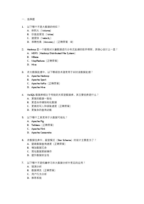
一、选择题1.以下哪个不是大数据的特征?A.体积大(Volume)B.价值密度低(Value)C.速度快(Velocity)D.准确性高(Accuracy)(正确答案:D)2.Hadoop是一个能够对大量数据进行分布式处理的软件框架,其核心设计之一是?A.HDFS(Hadoop Distributed File System)B.HBaseC.MapReduce(正确答案)D.Hive3.在大数据处理中,以下哪项技术通常用于实时流数据处理?A.Apache HadoopB.Apache SparkC.Apache Kafka(正确答案)D.Apache Hive4.NoSQL数据库相比于传统的关系型数据库,其主要优势是什么?A.更强的数据一致性B.更适合存储结构化数据C.更高的写入和读取速度(正确答案)D.更复杂的查询功能5.以下哪个工具常用于大数据可视化?A.Apache PigB.Tableau(正确答案)C.Apache FlinkD.Apache Cassandra6.在数据仓库中,星型模式(Star Schema)的设计主要是为了?A.提高数据查询速度(正确答案)B.增加数据冗余C.简化数据更新操作D.提升数据安全性7.以下哪个不是机器学习在大数据分析中常见的应用?A.预测分析B.数据清洗(正确答案)C.用户行为分析D.推荐系统8.在进行大数据处理时,数据科学家通常使用哪种语言进行数据处理和分析?A.JavaB.Python(正确答案)C.C++D.JavaScript。
- 1、下载文档前请自行甄别文档内容的完整性,平台不提供额外的编辑、内容补充、找答案等附加服务。
- 2、"仅部分预览"的文档,不可在线预览部分如存在完整性等问题,可反馈申请退款(可完整预览的文档不适用该条件!)。
- 3、如文档侵犯您的权益,请联系客服反馈,我们会尽快为您处理(人工客服工作时间:9:00-18:30)。
Star Schema Benchmark Revision 3, June 5, 2009Pat O'Neil, Betty O'Neil, Xuedong Chen{poneil, eoneil, xuedchen}@UMass/Boston1. Star Schema Based on TPC-H This section provides an explanation of design deci-sions made in creating the Star Schema benchmark or SSB. The SSB is designed to measure performance of database products in support of classical data ware-housing applications, and is based on the TPC-H benchmark [TPC-H], modified in a number of ways explained in this section.Here are a few ground rules. First, the columns in the SSB tables can be compressed by whatever means available in the database system used, as long as re-ported data retrieved by queries has the values specified in our schemas: e.g., we report values: Monday, Tues-day, ..., Sunday, rather than 1, 2,..., 7. Second, the au-thors are not attempting to make this benchmark bullet-proof by listing illegal tuning approaches. However, any product capability used in one product database de-sign to improve performance must be matched in the database design for other products by an attempt to use the same type of capability, assuming such a capability exists and improves performance.In outline, here are some of the schema changes we use to change the Normalized TPC-H schema (see Figure 1.1) to the efficient star schema form of SSB (see Fig-ure 1.2). Many reasons for these changes are taken from [Kimball], q.v. More detailed explanations of changes will be provided in Section 2.1. We combine the TPC-H LINEITEM and ORDERS tables into one sales fact table that we name LINEORDER. This denormalization is standard in wa-rehousing, as explained in [Kimball], pg. 121, and makes many joins unnecessary in common queries.2. We drop the PARTSUPP table since it would belong to a different data mart than the ORDERS and LINEITEM information. This is because PARTSUPP has different temporal granularity, as explained in Sec-tion 2.1.3. We drop the comment attribute of a LINEITEM (27 chars), the comment for an order (49 chars), and the shipping instructions for a LINEITEM (25 chars), be-cause a warehouse does not store such information in a fact table (they can’t be aggregated, and take signifi-cant storage). See [Kimball], pg. 18. Note this change tendsLI N E OR DER (LO_) P AR T (P_)C U S TO M E R(C_)Figure 1.2 SSB Schemato favor row stores, but is appropriate based on ware-house design principles.6. We add the DATE dimension table, as is standard for a warehouse on sales.The result of the table simplifications is a proper star schema data mart, with LINEORDER as a central fact table and dimension tables for customer, part, supplier, and date. A series of tables for shipdate, receiptdate, and returnflag, as mentioned in point 5, above could al-so be constructed, but would result in too complicated a schema for our simple star schema benchmark.As regards queries we support in SSBM, we concen-trate on queries that select from the LINEORDER table exactly once (no self-joins or subqueries or table que-ries also involving LINEORDER). The classic ware-house query selects from the fact table with restrictions on the dimension table attributes. We also support que-ries that appear in TPC-H and restrict on fact table attributes. We depart from the TPC-H query format for a number of reasons, most commonly to make an at-tempt to provide the Functional Coverage and Selectiv-ity Coverage features explained in [SETQ]. Functional Coverage. The benchmark queries are cho-sen as much as possible to span the tasks performed by an important set of Star Schema queries, so that pros-pective users can derive a performance rating from the weighted subset they expect to use in practice.It is difficult to provide true functional coverage with a small number of queries, but we at least try to provide queries that have 1, 2, 3, and 4 dimensional restrictions. Selectivity Coverage. The idea here is that the total number of fact table rows retrieved will be determined by the selectivity (i.e., total Filter Factor FF) of restric-tions on dimensions. We wish to vary this selectivity from queries where a lot of fact table rows are retrieved (though the data reported out is normally aggregated) to queries where a relatively small number of rows are re-trieved.The SSBM Queries are specified in Section 3.1, and a short analysis showing how multiple sort-orders for LINEORDER will make for efficient queries is pro-vided in Section 3.1.One other issue arises in running the Star Schema Benchmark queries, and that is the caching effect that reduces the number of disk accesses necessary when query Q2 follows query Q1, because of overlap of data accessed between Q1 and Q2. The approach we will try to take is to minimize this overlap. In situations where this cannot be done, if such arise, we will take whatever steps are needed to reduce caching effects of one query on another. Reporting requirements for SSBM are covered in Sec-tion 5: we will want to report lots of things: query plans, numbers of rows accessed, CPU time in queries, disk I/O, etc.2. Detail on SSB FormatIn this section, we will specify the schemas of the vari-ous tables to be used in the Star Schema. Note that in Appendix A, we provide a listing of the original TPC-H tables on which the definitions that follow are based.2.1 We drop the PARTSUPP tableHere is an argument why this is appropriate, based on principles in [KIMBALL]. The problem is that the LINEITEM and ORDERS tables (combined in SSBM to make a LINEORDER table) have the finest Transac-tion Level temporal grain, while the PARTSUPP table has a Periodic Snapshot grain. This means that transac-tions that add new rows over time to LINEORDER do not modify rows in PARTSUPP, which is frozen in time (presumably at the CURRENT date).This would be fine if PARTSUPP and LINEORDER were treated as SEPARATE FACT TABLES (i.e., sep-arate Data Marts in terms of Kimball), queried sepa-rately and not joined together. This is done in all but one of the Queries where PARTSUPP is in the WHERE clause: Q1, Q11, Q16 and Q20, but not in Q9, where PARTSUPP, ORDERS, and LINEITEM all ap-pear. Query Q9 is intended to find, for each nation and year, the profits for certain parts ordered that year. Profit is calculated as sum of [(l_extendedprice*(1 -l_discount) - (ps_supplycost*l_quantity)], and the sum is grouped by the o_orderdate for the LINEITEM col-umns and the s_nationkey for the part supplied to the order by the PARTSUPP table.The problem, of course, is that it is beyond the bounds of reason that the ps_supplycost would have remained constant during all these past years. This difference in grain between PARTSUPP and LINEORDER is what causes the problem.The presence of a Snapshot PARTSUPP table in this design seems suspicious anyway, as if placed there to require a non-trivial normalized join schema; it is very much what we would expect in an update transactional design, where in adding an order LINEITEM for some part, we would access PARTSUPP to find the minimal cost supplier, perhaps in some restricted region, and would then correct ps_availqty after filling the order. In the TPC-H benchmark, however, ps_availqty is never updated, not even during the Refresh that inserts new ORDERS. In a Star Schema data warehouse, it's more reasonable to leave out the PARTSUPP table, and create a column supplycost for each LINEORDER Fact row to answer such questions. A data warehouse, ofcourse, contains derived data only, so there is no reason to normalize to guarantee one fact in one place -- the next order for the same part and supplier might repeat this price, and if we delete the last part of some kind we might lose the price charged, but that's fine since we're trying to simplify queries. In fact, we add the lo_profit column to the LINEORDER table to simplify calcula-tions of this type even further. In general, there are a number of modifications.See Appendix A for listing of Original TPC-H Table Layouts. Note that all tables in TPC-H and SSB scale from a given size at Scale Factor 1 (SF = 1) to 10 times as large (for example) at SF = 10. Typically tables have cardinalities that are multiples of SF (but see the Part table, Section 2.3 in what follows).2.2 Layout of LINEORDER Fact table.We combine the LINEITEM and ORDERS tables into one sales fact table that we name LINEORDER. This denormalization is standard in warehousing, as ex-plained in [Kimball], pg. 121, and makes many joins unnecessary in common queries. Columns are classi-fied as identifiers (any datatype but unique values for what it is identifying), text (fixed or variable length), and numeric (whole numbers, not floating point.) Nu-meric identifiers must have unique values and have numeric interpretations which provide unique numbers. Text is in 8-bit ASCII. For numeric columns, the needed range of numbers is indicated.LINEORDER Table Layout SF*6,000,000LO_ORDERKEY numeric (int up to SF 300) first 8 of each 32 keys populatedLO_LINENUMBER numeric 1-7LO_CUSTKEY numeric identifier FK to C_CUSTKEY LO_PARTKEY identifier FK to P_PARTKEYLO_SUPPKEY numeric identifier FK to S_SUPPKEY LO_ORDERDATE identifier FK to D_DATEKEY LO_ORDERPRIORITY fixed text, size 15 (See pg 91: 5 Priorities: 1-URGENT, etc.)LO_SHIPPRIORITY fixed text, size 1LO_QUANTITY numeric 1-50 (for PART)LO_EXTENDEDPRICE numeric ≤ 55,450 (for PART) LO_ORDTOTALPRICE numeric ≤ 388,000 (ORDER) LO_DISCOUNT numeric 0-10 (for PART, percent) LO_REVENUE numeric (for PART:(lo_extendedprice*(100-lo_discnt))/100)LO_SUPPLYCOST numeric (for PART)LO_TAX numeric 0-8 (for PART)LO_COMMITDATE FK to D_DATEKEYLO_SHIPMODE fixed text, size 10 (See pg. 91: 7 Modes: REG AIR, AIR, etc.)Compound Primary Key: LO_ORDERKEY,LO_LINENUMBER NOTES. (a) We drop all columns in ORDERS and LINEITEMS that make us wait to insert a Fact row af-ter an order is placed on ORDERDATE, For example, we don't want to wait until we know when the order is shipped, when it is received, and whether it is returned before we can query the existence of an order: see pg 96 and 97 of the TPC-H Specification. Thus we drop L_RETURNFLAG, L_LINESTATUS, L_SHIPDATE, L_RECEIPTDATE, and O_ORDERSTATUS. We keep L_COMMITDATE since that is the delivery date promised to the customer at ship time. (b) We dropO_COMMENT (text string [49]), L_COMMENT (text string[27]), and L_SHIPINSTRUCT (text string [25]), since data warehouse queries typically do not parse comments and cannot aggregate them; similarly we drop LO_CLERK (text string[15]); columns such as these are only useful in an operational venue, though some abstraction of this information might well be made available in a data warehouse in a form where a query can return quantitative results. (c) We also add LO_SUPPLYCOST for PART,LO_ORDSUPPLYCOST summing for ORDERS, and bring over O_TOTALPRICE asLO_ORDTOTALPRICE.2.3 Layout of Part Dimension Table. New cardinality growth relative to SF (logarithmic)PART Table Layout 200,000*floor(1+log2SF)P_PARTKEY identifierP_NAME variable text, size 22 (Not unique)P_MFGR fixed text, size 6 (MFGR#1-5, CARD = 5) P_CATEGORY fixed text, size 7 ('MFGR#'||1-5||1-5: CARD = 25)P_BRAND1 fixed text, size 9 (P_CATEGORY||1-40: CARD = 1000)P_COLOR variable text, size 11 (CARD = 94)P_TYPE variable text, size 25 (CARD = 150)P_SIZE numeric 1-50 (CARD = 50)P_CONTAINER fixed text, size 10 (CARD = 40) Primary Key: P_PARTKEYNOTES. (a) P_NAME is as long as 55 bytes in TPC-H, which is unreasonably large. We reduce it to 22 by li-miting to a concatenation of two colors (see [TPC-H], pg 94). We also add a new column named P_COLOR that could be used in queries where currently a color must be chosen by substring from P_NAME. (b)P_MFGR is fixed text, size 25 in TPC-D; we change the values to ["MFGR",M], where M = random value [1,5], e.g.: "MFGR#2", a total of 6 characters. (c) We add a new column P_CATEGORY as a division ofP_MFGR (to take the place of P_BRAND in [TPC-H], which has 25 values, an unreasonably small number of brands; we add a new column P_BRAND1, a division of P_CATEGORY (see [KIMBALL], pg 21, paragraph 3: P_CATEGORY might be 'Paper Products' andP_BRAND1 is a true Brand such as 'Snap-On'). (d) We drop P_RETAILPRICE (this is likely to change too frequently to be in a dimension; the part price is better determined for an order many days old asLO_EXTENDEDPRICE/LO_QUANTITY. (e) We drop P_COMMENT; as with O_COMMENT, we have no use for an unparsed comment in a data warehouse query. (f) While PARTS (or PRODUCTS) typically form a large dimension, they do not grow so fast that they remain in the ratio 2/15 to the number of rows in a large ORDERS table (as they would with SF*200,000 rows). Thus we change the scaling factor to200,000*floor(1+log2SF). There will be 200,000 parts for 6,000,000 LINEORDER rows (SF =1), jumping to 400,000 parts when there are 12,000,000 LINEORDER rows (SF = 2), to 600,000 parts when there are24,000,000 LINEORDER rows (SF = 4), and so on. Note that sublinear scaling is also a feature of the planned benchmark presented in [TPC-DS].2.4 Layout of Supplier Dimension Table. SUPPLIER Table Layout (SF*2,000 are populated):S_SUPPKEY numeric identifierS_NAME fixed text, size 25: 'Supplier'||S_SUPPKEY S_ADDRESS variable text, size 25 (city below)S_CITY fixed text, size 10 (10/nation:S_NATION_PREFIX||(0-9)S_NATION fixed text, size 15 (25 values, longest UNITED KINGDOM)S_REGION fixed text, size 12 (5 values: longest MIDDLE EAST)S_PHONE fixed text, size 15 (many values, format: 43-617-354-1222)Primary Key: S_SUPPKEYNOTES. (a) We reduce the number of suppliers so as to not have too many suppliers per customer. (b) TheS_CITY column is created using the first 9 characters of the S_NATION (blank extended if there are fewer than 9) followed by a digit 0-9. This column is added because there is no other column that can be restricted to result in a reasonably small filter factor, an unnatural situation in real applications.2.5 Layout of Customer Dimension Table. CUSTOMER Table Layout (SF*30,000 are populated) C_CUSTKEY numeric identifierC_NAME variable text, size 25'Cutomer'||C_CUSTKEYC_ADDRESS variable text, size 25 (city below)C_CITY fixed text, size 10 (10/nation:C_NATION_PREFIX||(0-9)C_NATION fixed text, size 15 (25 values, longest UNITED KINGDOM) C_REGION fixed text, size 12 (5 values: longest MIDDLE EAST)C_PHONE fixed text, size 15 (many values, format: 43-617-354-1222)C_MKTSEGMENT fixed text, size 10 (longest is AUTOMOBILE)Primary Key: C_CUSTKEYNOTES. (a) We drop C_ACCTBAL, which does not match the grain of LINEORDER. (b) With SF*150,000 customers and 1,500,000 orders, this means we expect the average customer to place 10 orders in 7 years, an unreasonably small number. We change the number of customers to SF*30,000, or 50 orders in 7 years, about 7 orders a year.2.6 Layout of (NEW) Date Dimension Table. DATE Table Layout (7 years of days)D_DATEKEY identifier, unique id -- e.g. 19980327 (what we use)D_DATE fixed text, size 18: e.g. December 22, 1998 D_DAYOFWEEK fixed text, size 8, Sunday..Saturday D_MONTH fixed text, size 9: January, ..., December D_YEAR unique value 1992-1998D_YEARMONTHNUM numeric (YYYYMM)D_YEARMONTH fixed text, size 7: (e.g.: Mar1998D_DAYNUMINWEEK numeric 1-7D_DAYNUMINMONTH numeric 1-31D_DAYNUMINYEAR numeric 1-366D_MONTHNUMINYEAR numeric 1-12D_WEEKNUMINYEAR numeric 1-53D_SELLINGSEASON text, size 12 (e.g.: Christmas) D_LASTDAYINWEEKFL 1 bitD_LASTDAYINMONTHFL 1 bitD_HOLIDAYFL 1 bitD_WEEKDAYFL 1 bitPrimary Key: D_DATEKEYNOTES.(a) For source of Date columns, see [Kimball] page 39. We leave out Fiscal dates. (b) Note that we keep the DATE dimension in order by date.3. Benchmark QueriesAs in the Set Query Benchmark [O'NEIL93], we strive in this benchmark to provide functional coverage (dif-ferent common types of Star Schema queries) and Se-lectivity Coverage (varying fractions of the LINEITEM table that must be accessed to answer the queries). We only have a small number of flights to use to provide such coverage, but we do our best. Some model queries will be based on the TPC-H query set, but we need to modify these queries to vary the selectivity, resulting in what we call a Query Flight below. Other queries that we feel are needed will have no counterpart in TPC-H.In Section 3.1, we provide the definitions of queries we propose to use in SSBM. Section 3.1 provides a bit of analysis of the benchmark, including an indication of multiple sortorders for LINEITEM that will provide best efficiency.3.1 Query DefinitionsMany queries in TPC-H will not translate into our schema. For example, TPCQ1 requires knowledge of all items shipped as of a given date and whether these items were returned. We have decided that our LINEORDER table will only have ordering informa-tion, and that other data marts would be needed for shipping, receipt, and return information (see [KIMBALL], pg. 94). Similarly, TPCQ2 asks for the minimum cost supplier for parts in various regions, which requires the PARTSUPP table (assuming it's up-to-date). TPCQ3 requires knowledge that an order is unshipped, TPCQ4 requires knowledge of receipt date by customer. And so on. Only a few queries from TPC-H can be implemented on our SSBM scheme with mi-nimal modification.Here are the (Draft) query flights we propose.Q1. We want to start with a query flight having restric-tions on only one dimension. We base Q1 on TPC-H query TPCQ6, which has rather unusual restrictions on the Fact table as well; however the rationale for these Fact table restrictions seems reasonable. The query is meant to quantify the amount of revenue increase that would have resulted from eliminating certain company-wide discounts in a given percentage range for products shipped in a given year. This is a "what if" query to find possible revenue increases. Since our lineorder ta-ble doesn't list shipdate, we will replace shipdate by or-derdate in the flight.Q1 select sum(lo_extendedprice*lo_discount) as reve-nuefrom lineorder, datewhere lo_orderdate = d_datekeyand d_year = [YEAR] -- Specific values belowand lo_discount between [DISCOUNT] - 1and [DISCOUNT] + 1 and lo_quantity <[QUANTITY];In TPC-H: d_year = [YEAR], random year in [1993..1997] FF = 1/7, lo_quantity < [QUANTITY] a random quantity in [24..25], FF ≈ 47/100, lo_discount value [DISCOUNT] random [2..9], FF = 3/11In our Q1 Query flight we will restrict lo_quantity, not just to the lower half of the range, but to different ranges with different filter factors. Query flight Q1 has three queries. Q1.1 YEAR = 1993, DISCOUNT = 2, QUANTITY = 25, so predicates are d_year = 1993, lo_quantity < 25, lo_discount between 1 and 3.select sum(lo_extendedprice*lo_discount) as revenue from lineorder, datewhere lo_orderdate = d_datekeyand d_year = 1993and lo_discount between1 and 3and lo_quantity < 25;FF = (1/7)*0.5*(3/11) = 0.0194805. Number of li-neorder rows selected, for SF = 1, is0.0194805*6,000,000 ≈ 116,883.Q1.2 d_yearmonthnum = 199401, lo_quantity between 26 and 35, lo_discount between 4 and 6.select sum(lo_extendedprice*lo_discount) as revenue from lineorder, datewhere lo_orderdate = d_datekeyand d_yearmonthnum = 199401and lo_discount between4 and 6and lo_quantity between 26 and 35;FF = (1/84)*(3/11)*0.2 = 0.00064935. Number of li-neorder rows selected, for SF = 1:0.00064935*6,000,000 ≈ 3896.Q1.3 d_weeknuminyear = 6 and d_year = 1994,lo_quantity between 36 and 40, lo_discount between 5 and 7.select sum(lo_extendedprice*lo_discount) as revenue from lineorder, datewhere lo_orderdate = d_datekeyand d_weeknuminyear = 6and d_year = 1994and lo_discount between 5 and 7and lo_quantity between 26 and 35;FF = (1/364)*(3/11)*0.1 = .000075. Number of li-neorder rows selected, for SF = 1, is.000075*6,000,000 ≈ 450.NOTE that each of the selections of these three queries is disjoint in lineorder and even in restrictions on col-umns, so there should be no overlap where caching might make results vary from cold access.Q2. For a second query flight, we want a query type with restrictions on two dimensions. Our query will compare revenue for some product classes, for suppli-ers in a certain region, grouped by more restrictive product classes and all years of orders; since TPC-H has no query of this description, we add it here.Q2.1: p_category = 'MFGR#12', s_region ='AMERICA'select sum(lo_revenue), d_year, p_brand1from lineorder, date, part, supplierwhere lo_orderdate = d_datekeyand lo_partkey = p_partkeyand lo_suppkey = s_suppkeyand p_category = 'MFGR#12'and s_region = 'AMERICA'group by d_year, p_brand1order by d_year, p_brand1;p_category = 'MFGR#12', FF = 1/25; s_region, FF=1/5. So LINEORDER FF = (1/25)*(1/5) = 1/125. Number of lineorder rows selected, for SF = 1, is(1/125)*6,000,000 ≈ 48,000Q2.2 Change p_category = 'MFGR#12' to p_brand1 be-tween 'MFGR#2221' and 'MFGR#2228' and s_region to 'ASIA'.select sum(lo_revenue), d_year, p_brand1from lineorder, date, part, supplierwhere lo_orderdate = d_datekeyand lo_partkey = p_partkeyand lo_suppkey = s_suppkeyand p_brand1 between'MFGR#2221' and 'MFGR#2228'and s_region = 'ASIA'group by d_year, p_brand1order by d_year, p_brand1;So lineorder FF = (1/125)*(1/5) = 1/625. Number of li-neorder rows selected, for SF = 1, is (1/625)*6,000,000 ≈ 9600.Q2.3 Change p_category = 'MFGR#12' to p_brand1 = 'MFGR#2339' and s_region = 'EUROPE'.select sum(lo_revenue), d_year, p_brand1from lineorder, date, part, supplierwhere lo_orderdate = d_datekeyand lo_partkey = p_partkeyand lo_suppkey = s_suppkeyand p_brand1 = 'MFGR#2221'and s_region = 'EUROPE'group by d_year, p_brand1order by d_year, p_brand1;So lineorder FF = (1/1000)*(1/5) = 1/5000. Number of lineorder rows selected, for SF = 1, is(1/5000)*6,000,000 ≈ 1200. One of the Group By clauses has only one value.NOTE again, each of the selections of these four que-ries is disjoint in lineorder and even in restrictions on columns among themselves and also with flight Q1, so there should be no overlap where caching might make results vary from cold access.Q3. In our third query flight, we want to place restric-tions on three dimensions, including the remaining di-mension, customer. We base our query on TPCQ5. The query is intended to provide revenue volume for li-neorder transactions by customer nation and supplier nation and year within a given region, in a certain time period.Q3 select c_nation, s_nation, d_year, sum(lo_revenue) as revenue from customer, lineorder, supplier, date where lo_custkey = c_custkeyand lo_suppkey = s_suppkeyand lo_orderdate = d_datekeyand c_region = 'ASIA' and s_region = 'ASIA'and d_year >= 1992 and d_year <= 1997group by c_nation, s_nation, d_yearorder by d_year asc, revenue desc;Q3.1 Q3 as written: c_region = 'ASIA' so FF = 1/5 for customer, FF = 1/5 for supplier, and 6-year period FF = 6/7 for d_year; Thus LINEORDER FF =(1/5)*(1/5)*(6/7) = 6/175 and the number of lineorder rows selected, for SF = 1, is (6/175)*6,000,000 ≈205,714.Q3.2 Change restriction to a certain nation, and within that nation, revenue by customer city and supplier city, and year.select c_city, s_city, d_year, sum(lo_revenue) as reve-nue from customer, lineorder, supplier, datewhere lo_custkey = c_custkeyand lo_suppkey = s_suppkeyand lo_orderdate = d_datekeyand c_nation = 'UNITED STATES'and s_nation = 'UNITED STATES'and d_year >= 1992 and d_year <= 1997group by c_city, s_city, d_yearorder by d_year asc, revenue desc;Here the c_nation and s_nation restriction has FF = (1/25); so lineorder FF is (1/25)*(1/25)*(6/7) = 6/4375. The number of lineorder rows selected, for SF = 1, is (6/4375)*6,000,000 ≈ 8,228.Q3.3 Change restriction to two cities in 'UNITED KINGDOM'; retrieve c_city and group by c_city. select c_city, s_city, d_year, sum(lo_revenue) as reve-nue from customer, lineorder, supplier, datewhere lo_custkey = c_custkeyand lo_suppkey = s_suppkeyand lo_orderdate = d_datekeyand (c_city='UNITED KI1'or c_city='UNITED KI5')and (s_city='UNITED KI1'or s_city=’UNITED KI5')and d_year >= 1992 and d_year <= 1997group by c_city, s_city, d_yearorder by d_year asc, revenue desc;Here the c_nation and s_nation restriction has FF = (2/10)(1/25)= 1/125; so lineorder FF is(1/125)*(1/125)*(6/7) = 6/109375. The number of li-neorder rows selected, for SF = 1, is(6/109375)*6,000,000 ≈ 329.Q 3.4 Drill down in time to just one month, to create a “needle-in-haystack” query.select c_city, s_city, d_year, sum(lo_revenue) as reve-nue from customer, lineorder, supplier, datewhere lo_custkey = c_custkeyand lo_suppkey = s_suppkeyand lo_orderdate = d_datekeyand (c_city='UNITED KI1' orc_city='UNITED KI5')and (s_city='UNITED KI1' ors_city='UNITED KI5')and d_yearmonth = 'Dec1997'group by c_city, s_city, d_yearorder by d_year asc, revenue desc;so lineorder FF is (1/125)*(1/125)*(1/84) =1/1,312,500. The number of lineorder rows selected, for SF = 1, is (1/1,312,500)*6,000,000 ≈ 5.NOTE again, each of the selections of these queries is disjoint in lineorder and also with flights Q1 and Q2, except for Q3.4 vs. Q 3.3, so there should be no over-lap where caching might make results vary from cold access, except for Q3.4.Q4. The following query flight represents a "What-If" sequence, of the OLAP type. We start with a group by on two dimensions and rather weak constraints on three dimensions, and measure the aggregate profit, meas-ured as (lo_revenue - lo_supplycost).select d_year, c_nation, sum(lo_revenue -lo_supplycost) as profit from date, customer, supplier, part, lineorderwhere lo_custkey = c_custkeyand lo_suppkey = s_suppkeyand lo_partkey = p_partkeyand lo_orderdate = d_datekeyand c_region = 'AMERICA'and s_region = 'AMERICA'and (p_mfgr = 'MFGR#1' or p_mfgr = 'MFGR#2') group by d_year, c_nationorder by d_year, c_nationQ4.1 Query Q4 as written. Restriction on region re-striction FFs 1/5 each, p_mfgr restriction 2/5. FF on li-neorder = (1/5)(1/5)*(2/5) = 2/125. So the number of lineorder rows selected for SF = 1 is (2/125)*6,000,000 ≈ 96000.Assume that in Q4.1 output we find a surprising growth of 40% in profit from year 1997 to year 1998, uniform across c_nation. (This need not be true in the data we actually examine.) We would probably want to pivot to group by year, s_nation and a further breakdown byp_category to see where the change arises.Q4.2 select d_year, s_nation, p_category,sum(lo_revenue - lo_supplycost) as profitfrom date, customer, supplier, part, lineorderwhere lo_custkey = c_custkeyand lo_suppkey = s_suppkeyand lo_partkey = p_partkeyand lo_orderdate = d_datekeyand c_region = 'AMERICA'and s_region = 'AMERICA'and (d_year = 1997 or d_year = 1998)and (p_mfgr = 'MFGR#1'or p_mfgr = 'MFGR#2')group by d_year, s_nation, p_categoryorder by d_year, s_nation, p_categoryThis has the same FF as Q4.1 except in time and ac-cesses 2/7 of the same lineorder data; for that data it simply has a different group by dimension breakout. Its FF = (2/7)*(2/125) = 4/875. So the number of lineorder rows selected for SF = 1 is (4/875)*6,000,000 ≈27,428.Assume that as a result of Q4.2, a great percentage of the profit increase from year 1997 to 1998 comes from s_nation = 'UNITED STATES' and p_category ='MFGR1#4'. Now we might want to drill down to cities in the United States and into p_brand1 (withinp_category).Q4.3 select d_year, s_city, p_brand1, sum(lo_revenue - lo_supplycost) as profitfrom date, customer, supplier, part, lineorderwhere lo_custkey = c_custkeyand lo_suppkey = s_suppkeyand lo_partkey = p_partkeyand lo_orderdate = d_datekeyand c_region = 'AMERICA'and s_nation = 'UNITED STATES'and (d_year = 1997 or d_year = 1998)and p_category = 'MFGR#14'group by d_year, s_city, p_brand1order by d_year, s_city, p_brand1The FF for c_region is 1/5. and for s_nation is 1/25; the FF for d_year remains at 2/7, and the restriction onp_category is now 1/25. Thus the lineorder FF is:(1/5)*(1/25)*(2/7)*(1/25) = 2/21875. The number of。