基于Geomagic Studio的曲面重构过程
三维CAD模型重构方法、过程及实例
特征的定义及表达
几何特征是几何造型的关键,他们对控制几何形体的形状 有极为重要作用,同时几何特征之间还具有确定的几何约束 关系。
因此,在产品模型的重构过程中,一个重要的目标就是 还原这些特征以及他们之间的约束,得到一个优化的CAD模型, 使孤立的曲面片转化成一个整体的几何模型。
三维CAD模型重构方法、 过程和实例
输出匹配的 文件格式
自动将点云 数据转换为
多边形
Geomagic Studio
主要功能
快速减少 多边形数目
(Decimate)
曲面分析 (公差分析等)
把多边形 转换为曲面
三维CAD模型重构方法、 过程和实例
Geomagic Studio软件工作流程如下图所示:
这和多数工业产品的设计意图相符合。可有效解决产品 的装配对齐、造型的对称等问题,进而减小误差,提高产品 质量。
三维CAD模型重构方法、 过程和实例
约束的定义、分类及表达
逆向工程中的曲面重构不是对数据的简单拟合,而是 要满足几何约束下的重构。
三维CAD模型重构方法、 过程和实例
Imageware 软件
• 应用曲线拟合造型的典型商用软件 • 广泛应用于汽车、航天、消费家电、模具、计算机零部
件等设计与制造领域。 • 软件包括以下几个模块:基础模块、点处理模块、曲线、
曲面模块、多边形造型模块、检验模块和评估模块。
三维CAD模型重构方法、 过程和实例
曲
面
模
模
型
型
评
重
价
建
实 体 模 型
下 游 应 用
三维CAD模型重构方法、 过程和实例
➢ 应用这种三边域曲面重构方法的典型商用软件是 Geomagic Studio软件。该软件可轻易地从扫描所得的 点云数据创建出完美的多边形模型和网格,并可自动 转换为 NURBS 曲面。
作业1111
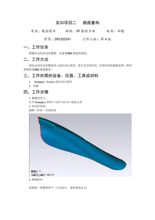
实训项目二曲面重构专业:数控技术班级:09数控3班姓名:郑魁学号:095305341 工作小组:第4组一、工作任务根据给定的多边形数据,完成NURBS曲面的重构。
二、工作方法将给定的多边形数据导入逆向设计软件,进行多边形阶段、形状阶段的数据处理,得到理想的NURBS曲面模型。
三、工作所需的设备、仪器、工具或材料1. Geomagic Studio逆向设计软件2. 电脑四、工作步骤1.数据的导入:打开Geomagic软件--文件--打开--选择文件2.多边形阶段:编辑—阶段—形状阶段3.探测曲率:轮廓线—探测曲率--(自动估计,曲率级别0.2)轮廓线—升级/约束--(调整最高曲率线且与边界相交,修改曲率线偏差部位)5.构造曲面片:曲面片—构造曲面片--(自动估计)6.曲面片调整:曲面片—调整—面板--(编辑,条)(定义,条)7.拟合轮廓线:轮廓线—拟合轮廓线--(选择中线,控制点2)--执行8.曲面片顶点修改:曲面片—编辑曲面片9.松弛轮廓线:轮廓线—松弛所有轮廓线10.松弛曲面片:曲面片—松弛曲面片—直线11.构造格栅:格栅—构造格栅--(分辨率20)12.拟合曲面:NURBS—拟合曲面--(常数,控制点6,默认表面张力0.25)五、思考题1、Geomagic Studio中,曲面重构工作过程可以划分为几个阶段?每个阶段完成的主要工作是什么?答:为3个阶段: 2、形状阶段:通过探测轮廓线和编辑轮廓线将之划分为多个面板;3、曲面片阶段:通过构造曲面片和移动面板等来实现曲面片的处理;4、NURBS曲面阶段:完成的曲面片进行构造栅格处理,拟合曲面后得到NURBS曲面。
2、松弛操作可以使模型表面平滑,如何控制松弛参数达到效果比较好的多边形模型?答:如果图形棱角比较突出,对图形进行松弛处理会使一些特征不明显,为了保留物体的原有轮廓特征,可以通过反选命令来处理,平滑级不应设置过大,强度在30左右3、多边形阶段边界处理对整个模型的质量具有重要作用,如何设置各项参数得到理想的边界(部分或者全部边界)?答:对于一些边界中多出的三角面片,我们选择删除,通过孔填充的方法处理填充,多余的删除,然后进行伸直,最后对整个边界进行松弛处理,小面积的通过砂纸打磨,达到美观边界的效果。
Geomagic系列教程 曲面的建立
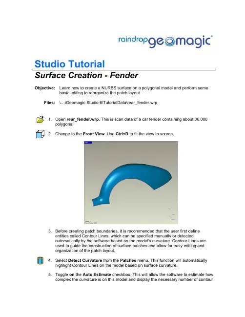
Studio TutorialSurface Creation - FenderObjective:Learn how to create a NURBS surface on a polygonal model and perform some basic editing to reorganize the patch layout.Files:\…\Geomagic Studio 6\TutorialData\rear_fender.wrp1. Open rear_fender.wrp.This is scan data of a car fender containing about 80,000polygons.2.Change to the Front View. Use Ctrl+D to fit the view to screen.3.Before creating patch boundaries, it is recommended that the user first defineentities called Contour Lines, which can be specified manually or detectedautomatically by the software based on the model’s curvature. Contour Lines areused to guide the construction of surface patches and allow for easy editing andorganization of the patch layout.4. Select Detect Curvature from the Patches menu. This function will automaticallyhighlight Contour Lines on the model based on surface curvature.5. Toggle on the Auto Estimate checkbox. This will allow the software to estimate howcomplex the curvature is on this model and display the necessary number of contourlines.6. Leave the Curvature Level set to the default of 0.3 and toggle on the SimplifyContour Lines checkbox. Click Apply.7.The orange line that appears among the black lines represents the line of highestcurvature on the model. This orange contour line is used to guide the softwareduring the next step, which is the automatic construction of rectangular surfacepatches.8. Click OK to exit the command. We will now manually select some of the black linesto turn them into additional contour lines, which will also help organize the patch layout when we get to the Construct Patches command in a few more steps.9. Select Promote/Constrain from the Patches menu. Start by left-clicking the blackentities shown below to promote them to orange contour lines. You model should resemble the image at right when complete. If you accidentally promote a line you did not want, hold down Ctrl and click on the line to demote it.10.Contour Lines are most effective when they form closed loops or start and end at theedge of the polygon model, as shown in the example at right, below. They helporganize the patch layout and result in a higher quality surface. A set of Contour Lines like the one shown below at left do not adequately define the features of the model or create closed loops and are therefore not very useful.Bad set of Contour Lines Good Set of Contour Lines11. Click OK to dismiss the dialog. You should now have a model divided into fivepanels, or regions bordered by contour lines. This will cause the software toconstruct boundaries within these panels.12. Select Construct Patches from the Patches menu. Again toggle on the AutoEstimate checkbox. This allows the software to determine approximately how many surface patches are needed to cover the surface of the polygon model.13. Toggle on Optimize Vertex Degree and click Apply. This function will automaticallyplace approximately 90 four-sided surface patches on the polygonalsurface…something no other software can do! And you can tell the software to place any number of patches on the surface, from 1 to 10,000!14.Notice the well-ordered nature of the patch layout. This is the benefit of usingcontour lines to define panels before using Construct Patches. At this point, the usercould complete the NURBS surfacing in two more easy steps. However, we will use this model to practice some basic editing of the patch layout first.15. Select Shuffle Panels from the Patches menu. Since our contour lines form closedregions, we can easily reshuffle them to create a more organized patch layout.16.Click anywhere on the large panel indicated below. When highlighted in white, clickthe four corners shown. Small red circles will appear after clicking each corner.¾ Quick Tip: It is best to zoom in and click just inside the panel when selecting the corners. This helps guarantee you have selected the right one17.After all four corners are picked, the model will appear as shown above. Thenumbers in red and green indicate the number of patches along each edge of the panel. When the numbers are green that means the number on the opposing side is the same, or balanced. When the numbers are red, they are different, orunbalanced. In order to shuffle this panel, opposing numbers must match. When both pairs of numbers match, the panel is balanced and can be automaticallyreorganized as an array, or grid, of patches.18. Change the Mode to Add 2 Paths. Click 2 times near the edge shown below tomake each side have 12 paths and balance the panel. You should have 4 paths on the short sides and 12 on the long sides of this panel.¾ Quick Tip:If you select the wrong path or corner, hit Ctrl+Z to undo the last pick.19.After adding the paths, both number pairs are balanced and colored green. Thismeans it is ready to be reshuffled. First, change the Type to Grid, if it is not already, which best describes this panel type. Then click Execute. The panel is reorganized in an orderly, grid-like fashion, as seen below. Note that with Auto Distributetoggled on, the vertices are also evenly distributed along each side when you click Execute.20. Click Next to shuffle another panel. Click on the long, skinny panel shown below andrepeat the process of defining corners, adding paths and distributing vertices toachieve the layout shown (2x2, 12x12). This time however, change the Type toStrip, since the Strip type is better suited for narrow, curving panels. Click Execute when the panel is balanced. It should appear as below.21.When satisfied with the layout, click Next to accept the changes and move to thenext panel.22.Continue making changes to the three smaller panels shown below until you havethe patch layout shown.23.When finished, click OK to exit the dialog.24.To straighten out a contour line that may be crooked, we can use tools like FitContour Line, which allow selective editing of contour lines.From the Patchesmenu, select Fit Contour Line.25.Select one of the contour lines, such as the one in the image below. Whenhighlighted, change the number of Control Points to 2. Hit Enter on your keyboard and a preview of the new fitting will be shown. Now click Execute to straighten the line. Results should appear as below, at right.26. Click OK to exit the command.27.You can also move individual vertices around manually. From the Patches menu,select Edit Patches.28.In the dialog, use the default setting, which is Move Vertices, and beginexperimenting with moving some of the control point vertices around by left-clicking one of the green points and dragging it to a new position. Notice that points always project onto the polygon surface. It is impossible to pull them off.29.Continue moving a few points around to get a feel for how easy it is to moveindividual vertices. This is one of the most useful editing tools in Shape Phase.30. Click OK when satisfied that you understand the function.31.It is easy to make changes to a well-ordered patch layout. We can, for example,quickly add or remove rows of patches in order to achieve our desired surfacequality.32. From the Patches menu, select Zip Patch Layers. Click on the line indicated below.A row of patches will become highlighted in white. Click Execute and that row ofpatches is removed, or “zipped”.33.Switch to the Unzip option. Click on the line indicated below. That row of patcheswill become highlighted in white. Click Execute. The selected row of patches is subdivided, or “unzipped”.34. Select OK to exit the dialog. This technique can be very useful if you require higheraccuracy on a particular portion of the model. Simply add one or two new rows of patches to achieve greater definition of the geometry.35. Click the Relax Contour Lines icon on the toolbar. This will help straighten out theContour Lines.36. Click the Relax Boundaries Linear icon, also on the toolbar. This helps evenlyspace the boundaries.37. Select Construct Grids from the Grids menu. Set the Resolution to 20 and clickOK. This operation places a U-V grid network inside each patch. The control points for our NURBS surface will follow these grids.¾ Quick Tip: The range for number of grids is 8-100. The higher the number, the more accurate the surface will be. Conversely, a lower number will tend to yielda smoother surface. A grid count between 20 and 50 is usually optimal. Thisvalue will not affect the file size of the final IGES file.38. Select Fit Surfaces from the NURBS menu. Set the Control Points value to 12 andthe Tension value to 0.25. Click OK. This operation automatically fits a C1continuous NURBS surface onto the grid network. Our surface is complete!39.To export an IGES or STEP surface, simply go to FileÆSave As and specify IGESor STEP as the type to save as.NOTE: IGES and STEP export are not possible with Evaluation versions ofGeomagic Studio. Contact your local Raindrop Geomagic representative if you wish to obtain the fully functional version, which allows the user to save in a wide variety of formats.End of Tutorial。
Geomagic逆向设计之参数化曲面设计
Geomagic Studio 12参数化设计案例之鼠标设计是一件非常愉快的事情,当你完成一个作品的时候,会有那么一点点成就感,但是同时,设计又是一件非常累的事情,一天超过8小时不停的点击鼠标,不仅是脑力劳动,更一个体力活。
那么,有没有什么方法可以更加便捷轻松的完成设计呢?答案当然是有了,我们在使用Proe,UG,CATIA,SOLIDWORKS做逆向设计的时候,可以与几个专业的逆向软件配合进行设计,如Geomagic,Rapdiform,polyworks,Imageware。
有些工作在这几款软件里面完成是比较方便快捷的,可以提高我们的设计效率。
下面就介绍一下使用Geomagic Studio12参数化曲面模块设计一款鼠标的流程。
Geomagic参数化曲面设计模块,如果是设计比较规则的机械零件,优势是不太明显的,但是像这款鼠标的设计,优势便比较明显了,设计效率高于UG、PROE等正向设计软件,简单快速。
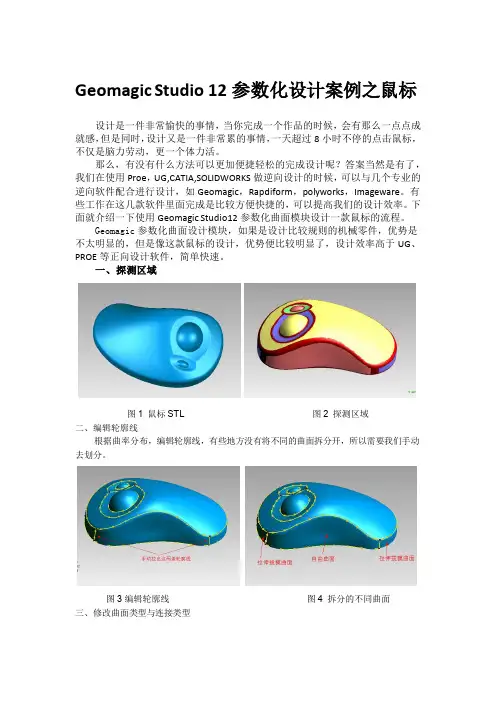
一、探测区域图1 鼠标STL 图2 探测区域二、编辑轮廓线根据曲率分布,编辑轮廓线,有些地方没有将不同的曲面拆分开,所以需要我们手动去划分。
图3 编辑轮廓线图4 拆分的不同曲面三、修改曲面类型与连接类型鼠标曲面大部分为粉红色自由曲面,绿色为球面,侧边由蓝色的拉伸拔模曲面与自由曲面组成。
黄色轮廓线为自由形态连接,蓝色轮廓线为固定半径连接面。
修改好曲面与连接类型后进去曲面拟合阶段。
图5 曲面与连接类型四、拟合曲面首先拟合主曲面,再拟合连接面。
拟合的主曲面出现一个桔红色错误曲面,我们手动编辑一下它的剖面,曲面更新后变为银白色高质量曲面。
图6 桔红色错误曲面图7 剖面线偏差太大图8 修改剖面线图9 主曲面五、拟合连接面拟合连接面后,发现有两个地方的R角存在问题,我们需要手动修改,编辑R角边界,重新生成连接面。
图10 问题R角连接面图11编辑R角边界图12 更新连接面六、拟合裁剪曲面总结:此案例的设计时间约20分钟。
基于Geomagic的摩托车零件海量点数据快速构建曲面的方法研究
利 用Gema i ̄大 的 海 量 点数 据 能 创造 出较 准确 的 o gc
目前 ,逆 向工程 技 术 在 金 城 集 团摩 托 车 、航 空 产 品 等 开发 设计 中愈 来愈 发挥 着重要 的 作用 ,而 逆 向工 程 中最 重要的 环节 仍是 构造 复杂 的 曲面 ,该环 节需要 花 费大量 的 时 间Ⅲ,特 别是 对一 些并 不 需要 产 品开 模 ,只需 要 产 品简
e u ig t e eo ns rn d v lpme t y l f e p o u t ndi r vngt ewo k e c e c . he n ceo n w r d csa mp o i h r f in y c i
Ke o d y w r s: Re e s l ngn ei g Daap o e sn Ra i e o sr c in o u e u fc v r a e ie rn t r c si g p dr c n tu t fc r ds ra e o v Ge m a i ATOS o gc
WuD n h a Yn a i Y n ig X a ag o L a (n hn ru o Ld o gu ig i n B q g a gQn io i u i n J cegG o pC . t. Jn Y i , )
Abs r c : Th e hn l g h tc nsr t ie ty t e c ve u f c p l ng t o l u ft e ta t e t c o o y t a o tucs d r c l h ur d s r a e a p yi he d tc o d o h Ge m a i o t a ep o i e e d sg o i e ai n a d am eh d f rt v lpm e to e p o u t, o g c s fw r r v d sa n w e in c nsd r to n t o o hede e o n fn w r d c s e p ca l rt h e — i e so a e i n oft e pat fc m plt f het r e dm n i n ld sg rso o yo h ee m t r y l p a a c .Fo h s rs rt o epa t ne dng no e d e , nl h i p e t r e dm e so a aa o h o ucsw h c sf rgetn he t o e i tn w i s o y t e sm l h e — i n i n ld t ft e pr d t i h i ti g t w - o d m e so a h c i r wi g , rc nd c ig t ev r la s m b y o t r y l a t o c c h n ef r n e i n i n lc e kngd a n s o o u t h it s e l fmo o c cep rst he k t ei tree c n ua b t e n t e p rswil e e o g o q c y c n tu tt e c m p iae u v d a pe r n e ew e h a l b n u h t uikl o sr c h o t lc t d c r e p a a c ,wh c i p i e h ih sm lf st e i w o k fo a d r ie her s n i e s e ip i g t e i tre e c t e h o o c c epat , h r w n a s st e po sbl pe d ofd s osn h n e fr n e bewe n t e m t r y l rs t us l
Geomagic Studio 11建立基本曲面
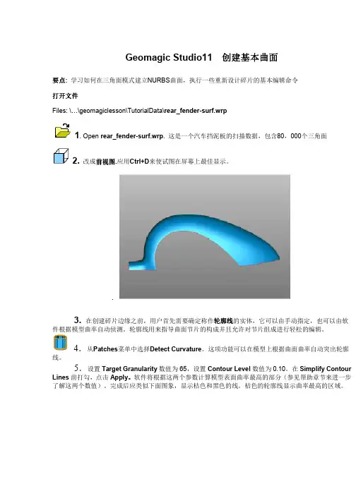
Geomagic Studio11 创建基本曲面创建基本曲面要点: 学习如何在三角面模式建立NURBS曲面,执行一些重新设计碎片的基本编辑命令打开文件Files: \ \geomagiclesson\TutorialData\rear_fender-surf.wrp1. Open rear_fender-surf.wrp. 这是一个汽车挡泥板的扫描数据,包含80,000个三角面2.改成前视图前视图.应用Ctrl+D来使试图在屏幕上最佳显示。
.3. 在创建碎片边缘之前,用户首先需要确定称作轮廓线轮廓线的实体,它可以由手动指定,也可以由软轮廓线件根据模型曲率自动侦测。
轮廓线用来指导曲面节片的构成并且允许对节片组成进行轻松的编辑。
4.从Patches菜单中选择Detect Curvature。
这项功能可以在模型上根据曲面曲率自动突出轮廓线。
5.设置Target Granularity数值为65,设置Contour Level数值为0.10。
在Simplify Contour Lines前打勾,点击Apply。
软件将根据这两个参数计算模型表面曲率最高的部分(参见帮助章节来进一步了解这两个数值)。
完成后应类似下面图象,显示桔色和黑色的线。
桔色的轮廓线显示曲率最高的区域。
6.点击OK关闭对话框。
你会注意到一条连续的桔色轮廓线穿过挡泥板的中心,我们现在手动选择一些黑色实体使他们变成额外的轮廓线。
7.从Patches菜单中选择Promote/Constrain命令。
开始点击下图所示五个黑色实体,使他们变成轮廓线。
完成后模型应如下正确显示。
小技巧::为了更方便选择线,使着用Rectangle或Paintbrush工具小技巧8.如果不小心选到了不想好的线,按住Ctrl并点击此线删除它。
小技巧小技巧::在三角面模型形成闭环或者边界的起终点时,轮廓线是最有效的。
单一的轮廓线不能确定零件形状。
9.点击OK关闭对话框,你现在可以看到模型被分成五部分,或者叫被轮廓线分成五个区域。
基于Geomagic Studio的叶片修复与曲面建模
部 有一 凹坑 , 现利 用 G o ai Sui em g tdo对其进 行 修复 , c 并 创建 曲 面模 型.
作用是获得整齐的划分 网格 , 而拟合成光顺 的曲 从
收稿 日期 : 0 10 —4 2 1— ll
基金项 目: 国家 自然科学基金资助项 目( 0 70 4 5 85 2 ) 广东 省教育部产学研结合项 目( 09 0 0 00 4) 广州 市科 技 5 7 54 ,0 0 0 5 ; 2 0 B 9 30 4 ;
形 阶段 和 曲面 阶段 J 点 阶段 主要 是 对 点 云 进 行 预 .
处理 , 括删 除 噪 点 、 云 采用 等 操 作 , 而 得 到 一 包 点 从 组整 齐 、 有序 的点 云 数据 . 多边 形 阶段 的主要 作 用 是 对 多边 形 网格数 据 进 行 表 面 光 顺 与 优 化 处理 , 以获
基 于 G o ai Su i 叶 片 修 复 与 曲面 建 模 em g tdo的 c
陈裕 芹 , 思源 , 成 邹付群 , 张湘伟
( 广东 工Байду номын сангаас 大学 机 电工程学 院, 广东 广州 50 0 ) 10 6
摘要 : 根据原始叶片扫描的点云数据 , 经过点 阶段 、 多边形 阶段 和曲面阶段 , 生成叶片的 C D模型. 利用 G o ai A 并 em g c
得 光顺 、 整 的三角 面片 网格 , 可 以消除错 误 的三 完 还
G o  ̄cSui ema tdo进行 缺陷 修复 之后 曲面 建模 .
2 叶片 曲面 建 模
如 图 2所 示 的 叶片模 型 , 上角 有一 折边 , 右 上半
角 面片 , 提高 后续 的 曲面重 建质 量 . 面阶段 包 含 两 曲 个模 块 : 状 模 块 和 Fsin模 块 . 状 模 块 的 主 要 形 aho 形
Geomagic Studio 12参数化曲面设计案例之机械零件
Geomagic Studio 12参数化曲面设计案例之机械零件Geomagic Studio 12.0参数化曲面模块擅长设计一些规则的机械零件,而不能设计由非倒圆的连续曲面构成的零件,因为没法处理曲面连续问题,不能设置曲面之间的相切连续与曲率连续,曲面之间的衔接只能使用倒圆处理。
以一标准零件为例,介绍Geomagic Studio 12参数化曲面模块的设计流程。
与精确曲面模块相同,网格数据不能有破洞,不能有锯齿的边界,因为设计出的曲面与stl数据会基本一致。
图 1 标准件(尺寸200mm×100mm×35mm)参数化曲面设计流程:探测区域(编辑轮廓线)——区域分类(编辑区域)——拟合曲面(编辑曲面、约束曲面)——拟合连接(分类连接)——裁剪缝合曲面图2 标准件STL数据详细步骤:1.探测轮廓实际就是拆面的过程,UG,PORE,CATIA的逆向设计都是手动拆面,每个设计师设计同一零件拆面的思路可能都一样,杰魔的拆面是根据零件的曲率拆分,自动计算其轮廓,生成轮廓线。
图3 探测轮廓 图4 提取轮廓线轮廓探测轮廓,抽取曲线以后,还需要对曲线进行编辑,补充或删除曲线,光顺曲线。
2.区域分类通过了探测区域,系统会自动拆面,不同的曲面类型赋予不同的颜色,例如平面为绿色,圆柱为黄色,拉伸为桔黄色等。
当然系统自动赋予的曲面类型不一定是我们需要的,因此当系统将一个拉伸面识别为一个自由曲面的时候,需要我们手动去改变该曲面的类型,这里我们把该曲曲由粉红色自由曲面修改为橘红色拉伸曲面。
要识别曲面是什么类型,需要我们有一定的曲面基础知识,还需要猜测设计者的设计意图。
杰魔里面的曲面可分为平面、圆柱、圆锥、拉伸、拉伸拔模、旋转、球、扫略、放样、自由形态。
图5 曲面分类 图6 修改错误的曲面类型3.拟合曲面修改曲面类型以后,便可以拟合主曲面,ctrl+A选取全部曲面,应用确定后还需要编辑曲面,修改圆柱直径,根据点云自动拟合的圆柱,直径数值一般不是相对整的数,如5.012mm,我们最初在设计的时候,不会出现这么多位的小数的,产生的这种误差来源于零件的加工误差以及点云拟合误差,我们可以根据实际情况保留小数点后1位的数值或直接取整。
Geomagic Studio最新曲面拼接教程
二、Geomagic Studio 11.0曲面拼接技术通过多次测量一个物体得到几块外形点云。
这几块独立点云需要拼接才能体显物体的完整形貌。
在拼接之前需要对单个点云进行一些处理,以保证后面的拼接顺利完成。
1.将测量获取的点云全部导入geomagic studio11.0指令:文件>导入图2-1 导入塑料件点云这是一个塑型工件,一共扫描了四幅,导入后如图所示。
2.删除点云的噪声点1)指令:左键选中第一幅点云,按快捷键“ATL+1”,只显示第一幅点云;2)指令: 点> Repair> 减少噪音结果如下所示:图2-2 删除噪点3.手动拼接指令:选中全部点云,工具>注册>手动注册;结果如下所示:图2-3 手动拼接4.精细拼接指令:选中全部点云,工具>注册>全局注册;图2-4 全局注册图2-5 拼接完成三、Geomagic Qualify11.0色谱比对以减震器质量检测为例,步骤如下:1.导入测试对象和参考对象。
如图3-1示指令:文件>导入图3-1 加载数据图3-2 对齐2.将测试对象和参考对象对齐。
如图3-2所示指令:选中测试对象,单击右键>设置为测试;选中参考对象,单击右键>设置为参考3.色谱误差分析指令:分析>3D比较图3-4 色谱分析4.创建注释指令:结果>创建注释图3-5 注释通过注释的创建可以看出在规定的公差范围内不合格的区域。
该实例中规定公差的范围为0.5mm~-0.5mm,注释中两个红色的区域偏差大于0.5mm,所以状态栏中显示“失败”。
5.GD&T标注指令:分析>GD&T>创建GD&T标注图3-6 GD&T标注GD&T及形位公差,可以标注零件的位置度、圆柱度、面轮廓度等等。
该参数有助于产品的趋势分析。
6.2D比较指令:分析>2D比较图3-7 2D尺寸标注a.YZ截面b.截面色谱图3-8 2D色谱比较7.创建报告指令:报告>创建报告可以创建的报告格式有:HTML,PDF,WORD,EXCEL,CSV。
利用Geomagic软件重建玩具模型过程中的曲面拟合实例①②-最新文档
利用Geomagic软件重建玩具模型过程中的曲面拟合实例①②1 概述逆向工程(Reverse Engineering,简称RE)也称为反向工程或反求工程,它是将实物转换为CAD模型的相关数字化技术、几何模型重建技术以及产品制造技术的总称[1],是缩短产品(尤其是形状复杂或具有自由曲面的产品)开发周期的一种有效途径,逆向工程的基本工作流程主要包括数据采集,数据预处理,数据分块,曲面拟合CAD 模型建立快速成型,其中曲面拟合本文借助玩具模型重点研究复杂曲面的曲面拟合过程。
该文中圣诞老人玩具模型的曲面拟合较为复杂,其研究主要集中在二个方面:一是建立由众多四边形组成的的曲面片模型;另一个是拟合NURBS曲面[2]。
逆向工程中多采用样条曲面对几何模型进行重构,把三角网格模型进一步表达为样条曲面的形式[3]。
该模型属于任意拓扑结构曲面模型,拟合的基本思路是首先重建散乱测量数据的拓扑结构,然后在此基础上对三角网格模型进行自动分片,一般是形成分片连续的四边界区域。
最后对分片区域采样,并根据边界光顺性构造边界条件,生成拟合曲面。
该方法的优点是自动化程度高,拓扑适应性强,生成的样条曲面拟合精度高,适合于该模型的曲面拟合。
2 曲面拟合与误差分析2.1 数据分块2.1.1 探测轮廓线选择菜单:“轮廓线―探测轮廓线”,设置曲率敏感性值为70.0,其他为默认值。
经过区域计算,生成如图1所示的红色曲率线。
从图中可明显观察到,模型生成的轮廓镶边十分不规整,需要在模型上增加或者减少轮廓镶边使其规整,便于后续操作。
经过对曲率线的轮廓镶边进行手动的修整,已基本使其变得规整。
如图2所示。
2.1.2 抽取轮廓线经过对轮廓线的手动修改后,进行下一步的操作:抽取轮廓线。
选中对话框中的“探测延伸轮廓线”多选框,设置“敏感性”为50.0,以便将所有的轮廓线都能变成黄色。
选中“检查路径相交”单选框,以便自动地检查是否有曲线相交。
单击“抽取”按钮,轮廓线被抽取出来。
- 1、下载文档前请自行甄别文档内容的完整性,平台不提供额外的编辑、内容补充、找答案等附加服务。
- 2、"仅部分预览"的文档,不可在线预览部分如存在完整性等问题,可反馈申请退款(可完整预览的文档不适用该条件!)。
- 3、如文档侵犯您的权益,请联系客服反馈,我们会尽快为您处理(人工客服工作时间:9:00-18:30)。
曲面重构处理流程
姓名:
学号:
班级:11材型(卓越)-1班
时间:2014年12月
目录
一、点处理阶段 (2)
二、多边形处理阶段 (7)
三、参数化曲面 (11)
一、点处理阶段
1. 打开素材文件。
启动Geomagic studio12软件后,点击→【打开】选择“swug3-1”文件如图。
图 1
2. 着色。
点击点工具栏的,系统将自动计算点云的法向量,赋予点云颜色。
图 2
3. 断开组件连接。
点击点工具栏的断开组件连接图标,弹出选择非连接选项的对话框,在“分隔”选择“低”,然后点击确定。
图 3
退出对话框后按Delete删除选中的非连接点云。
图 4
4. 选择体外孤点。
点击点工具栏的体外孤点图标,弹出体外孤点对话框,将敏感性设置为100。
图 5
点击应用后确定,按Delete删除选中的红色点云,该命令使用3次。
5. 手动删除。
点击矩形选择工具图标,进入矩形工具的选择状态,改变模型的视图(按住中间旋转),在视窗点击一个点,按住鼠标左键进行拖动框选,如图所示。
图 6
按Delete删除选中的红色杂点。
图 7
6. 减少噪音。
点击点工具栏的减少噪音图标,进入减少噪音对话框,点击应用后确定。
该命令有助于减少在扫描中的噪音点到最小,更好地表现真实的物体形状。
造成噪音点的原因可能是扫描设备轻微震动、物体表面较差、光线变化。
图 8
7. 统一采样。
点击点工具栏的统一采样图标,进入统一采样对话框,在输入中选择绝对间距里输入0.2mm,曲率优先拉到中间,点击应用后确定。
在保留物体原来面貌的同时减少点云数量,便于删除重叠点云、稀释点云。
图 9
8. 封装。
点击点工具栏的封装图标,进入封装对话框,直接点击确定,软件将自动计算。
该命令将点转换成三角面。
图 10
二、多边形处理阶段
1. 打开素材文件
启动Geomagic studio12软件后,点击图标,打开文件”swug4-2”。
图 12
2. 填充孔
点击多边形工具栏的选择填充单个孔图标,右键点击空白处,选择“选择边界”,再点击绿色边界,系统将选中边界并往内扩张(左键点击一次则扩展一次)。
按delete删除翘曲边界,右键选择“填充”,再手动去选择需填充的边界,最后按ESC退出命令。
图 13
3. 去除特征
点击蜡笔选择工具图标,进入蜡笔工具的选择状态,选择有问题的三角面,再点击多边形工具栏的去除特征图标,系统将自动根据红色周围的曲率变化进
行光顺。
4. 用平面进行裁剪
点击下的“用平面进行裁剪”,弹出“用平面进行裁剪“对话框。
定义选择“拾取边界”,选取边界,位置度设为2mm,点击“平面截面“按钮。
图 14
再点击“删除所选择”,删除底座下段区域,再点击“封闭相交面”,最后点击确定退出命令。
图 15
5. 网格医生
点击多边形工具栏下的网格医生图标,软件将自动选中有问题的网格面,点击应用后确定。
图 16
6. 删除钉状物
点击多边形工具栏下的删除钉状物图标,点击应用后确定。
该命令用于检测并展平多边形网格上的单点尖峰。
图 17
7. 松弛多边形
点击多边形工具栏下的松弛图标,将强度拉至第二格,点击应用后确定。
该命令用于最大限度减少单独多边形之间的角度,使多边形网格更加光滑。
图 18
8. 简化多边形
点击多边形工具栏下的简化图标,在减少到百分比栏输入70%,勾中“固定边界”,点击应用后确定。
该命令用于减少三角形数量但不影响其细节,勾中固定边界将在边界区域保留更多三角面。
图 19
9. 增强表面啮合
点击多边形工具栏下的增强表面啮合图标,点击应用后确定。
该命令用于在高曲率区域增加点而不破坏形状。
图 20
10. 保存三角面
保存STL文件,后期建模需要。
在左边管理器面板中右键点击“ Points”,选择“保存”,弹出保存对话框,输入文件名“swug7-2”,保存类型选择STL (binary)后,点击保存按钮。
三、参数化曲面
1. 打开素材文件
启动Geomagic studio12软件后,点击→【打开】选择“canshuhua1”文件。
图 21
2. 构造参数化曲面
点击参数化曲面工具栏下的构造参数化曲面图标,弹出对话框,点确定进行fashion阶段。
图 22
3. 检测区域
击参数化曲面工具栏下的检测区域图标,点击计算
图 23
系统将自动划分分隔符(曲率带),最后点击抽取完成对轮廓线的提取,点击确定退出命令。
若出现分隔符交叉则按住CTRL+蜡笔工具进行清理;若红色分隔符不均匀,必须使用蜡笔工具进行补选,有些未提取出来的高曲率带,可手动进行绘制。
图 24
合并相同的曲面:点击编辑栏的“合并面”图标,按住鼠标左键拖动并联合两块区域。
4. 编辑轮廓线
点击参数化曲面工具栏下的编辑轮廓线图标,勾选显示栏的“曲率图”,
拖动错误点到正确位置(高曲率带),若需增加节点,直接点击轮廓线并按ESC。
点击修改分隔符图标,点击更新分隔符,赋予新建轮廓线的分隔符。
最后点击确定退出命令。
若出现分隔符也参与构面,则重新检测区域,计算时点击“是”持先前的划分,再提取轮廓线,退出后将不会出现分隔符也参与构面。
图 25
5. 区域分类
先选中系统误认的区域,点击参数化曲面工具栏下的区域分类图标,重
新指定其曲面类型。
将中间凹面指定为回转面,部分侧面指定为拔模面,还有一个圆锥面,
6. 拟合曲面
先选中全部区域(全部拟合则Ctrl + A,全部不选则Ctrl + C),再点击参数化曲面工具栏下的拟合曲面图标。
点击“应用”后“确定”,弹出错误对话
框。
表示有些面拟合过程出现问题(误差较大的曲面用橘红色标识、有问题曲面用红色标识)。
图 26
7. 偏差
完成曲面构造后发现有块区域误差较大,点击参数化曲面工具栏的偏差图标,点击橘红色的曲面显示偏差。
图 27
8. 编辑剖面
由于该块区域误差较大,点击参数化曲面工具栏的编辑剖面图标,弹出横截线的拟合程度,黄色线为拟合线,两种蓝色线为点云线。
将线段密度调至最大,点击“应用”,发现曲线拟合的更加精确,但曲面仍显示误差较大,证明点云并非回转体,可能由扫描误差造成,需人为纠正,所以这里我们直接拟合回转球面就好。
9. 拟合连接
先选中需拟合的连接区域(全部拟合则Ctrl + A,全部不选则Ctrl + C),定义连接的类型:点击参数化曲面工具栏下的分类连接图标,指定所有连接为尖
锐角;再点击参数化曲面工具栏下的拟合连接图标,系统将自动拟合面与面之间的连接。
图 28
10. 修复曲面
先选中有问题的曲面(全部选择则Ctrl + A,全部不选则Ctrl + C),点击参数化曲面工具栏下的修复曲面图标,点击全部接受,最后点击确定退出对话框。
先不管倒圆出错的部分,在后续3D软件中进行再优化。
11. 修剪并缝合
选中所有曲面和连接(Ctrl + A),点击参数化曲面工具栏下的修剪并缝合图标,在生成对象中选择缝合曲面,点击应用后确定。
12. 保存文件
在左边管理器面板中右键点击“ point - 缝合模型”(CAD模型),选择“保存”,弹出保存对话框,输入文件名“point”,保存类型选择IGES或STEP文件后,点击保存按钮。