自动控制原理(中英文对照李道根)习题3题解
自动控制原理习题及其解答第三章

第三章例3-1 系统的结构图如图3-1所示。
已知传递函数 )12.0/(10)(+=s s G 。
今欲采用加负反馈的办法,将过渡过程时间t s减小为原来的0.1倍,并保证总放大系数不变。
试确定参数K h 和K 0的数值。
解 首先求出系统的传递函数φ(s ),并整理为标准式,然后与指标、参数的条件对照。
一阶系统的过渡过程时间t s 与其时间常数成正比。
根据要求,总传递函数应为)110/2.0(10)(+=s s φ即HH K s K s G K s G K s R s C 1012.010)(1)()()(00++=+= )()11012.0(101100s s K K K HHφ=+++=比较系数得⎪⎩⎪⎨⎧=+=+1010110101100H HK K K 解之得9.0=H K 、100=K解毕。
例3-10 某系统在输入信号r (t )=(1+t )1(t )作用下,测得输出响应为:t e t t c 109.0)9.0()(--+= (t ≥0)已知初始条件为零,试求系统的传递函数)(s φ。
解 因为22111)(ss s s s R +=+=)10()1(10109.09.01)]([)(22++=+-+==s s s s s s t c L s C 故系统传递函数为11.01)()()(+==s s R s C s φ 解毕。
例3-3 设控制系统如图3-2所示。
试分析参数b 的取值对系统阶跃响应动态性能的影响。
解 由图得闭环传递函数为1)()(++=s bK T Ks φ系统是一阶的。
动态性能指标为)(3)(2.2)(69.0bK T t bK T t bK T t s r d +=+=+= 因此,b 的取值大将会使阶跃响应的延迟时间、上升时间和调节时间都加长。
解毕。
例 3-12 设二阶控制系统的单位阶跃响应曲线如图3-34所示。
试确定系统的传递函数。
解 首先明显看出,在单位阶跃作用下响应的稳态值为3,故此系统的增益不是1,而是3。
自动控制原理课后习题答案

第1章控制系统概述【课后自测】1-1 试列举几个日常生活中的开环控制和闭环控制系统,说明它们的工作原理并比较开环控制和闭环控制的优缺点。
解:开环控制——半自动、全自动洗衣机的洗衣过程。
工作原理:被控制量为衣服的干净度。
洗衣人先观察衣服的脏污程度,根据自己的经验,设定洗涤、漂洗时间,洗衣机按照设定程序完成洗涤漂洗任务。
系统输出量(即衣服的干净度)的信息没有通过任何装置反馈到输入端,对系统的控制不起作用,因此为开环控制。
闭环控制——卫生间蓄水箱的蓄水量控制系统和空调、冰箱的温度控制系统。
工作原理:以卫生间蓄水箱蓄水量控制为例,系统的被控制量(输出量)为蓄水箱水位(反应蓄水量)。
水位由浮子测量,并通过杠杆作用于供水阀门(即反馈至输入端),控制供水量,形成闭环控制。
当水位达到蓄水量上限高度时,阀门全关(按要求事先设计好杠杆比例),系统处于平衡状态。
一旦用水,水位降低,浮子随之下沉,通过杠杆打开供水阀门,下沉越深,阀门开度越大,供水量越大,直到水位升至蓄水量上限高度,阀门全关,系统再次处于平衡状态。
开环控制和闭环控制的优缺点如下表1-2 自动控制系统通常有哪些环节组成?各个环节分别的作用是什么?解:自动控制系统包括被控对象、给定元件、检测反馈元件、比较元件、放大元件和执行元件。
各个基本单元的功能如下:(1)被控对象—又称受控对象或对象,指在控制过程中受到操纵控制的机器设备或过程。
(2)给定元件—可以设置系统控制指令的装置,可用于给出与期望输出量相对应的系统输入量。
(3)检测反馈元件—测量被控量的实际值并将其转换为与输入信号同类的物理量,再反馈到系统输入端作比较,一般为各类传感器。
(4)比较元件—把测量元件检测的被控量实际值与给定元件给出的给定值进行比较,分析计算并产生反应两者差值的偏差信号。
常用的比较元件有差动放大器、机械差动装置和电桥等。
(5)放大元件—当比较元件产生的偏差信号比较微弱不足以驱动执行元件动作时,可通过放大元件将微弱信号作线性放大。
自动控制原理(中英文对照李道根)习题2题解
2C ov
� � R� R � ) s( iVs 1C � )s ( oV� s 1C � � � )s ( A V �� � 1� 1 � )c( � R R R �� � )s ( oV � )s ( A V� s 2 C � �� � 1 1 2 �� ) s ( iV
.5.2P erugiF
) s ( 2 X 2 s 2 M � ]) s ( 2 X � ) s ( 1 X [ K
snቤተ መጻሕፍቲ ባይዱituloS■
�
)s ( F )s( 2 X
3
3 Z 1Z � 3 Z 2 Z � 2 Z 1Z
3Z0 Z
��
)s ( iV )s ( oV
�
�3 2Z 2 1 �� � Z � Z � Z �� ) s ( oV � ) s( A V� � 1 1 1 �� � 1 � )d( 1 0Z� Z � � ) s ( iV � 1 1 � )s ( A V
2 3
�
) s( R )s ( C
evah ew ,yaw emas a nI )b( si noitcnuf refsnart eht ,ecneH
� ) s( R )s ( C
evah ew ,snoitidnoc laitini orez gnimussa ,mrofsnart ecalpaL gnikaT )a( :noituloS
C
)1 � s (s 0K
5X 2K 2N
4X
sT 1
3X
2X
1G
1X
1N
R
.nwohs sa margaid kcolb eht evah ew , redro ni thgir ot tfel morf )s ( C dna )s ( 5 X , ) s ( 4 X , ) s( 3 X , ) s ( 2 X , )s ( 1 X , )s (R selbairav eht gnignarraeR
自动控制原理课后习题答案.docx
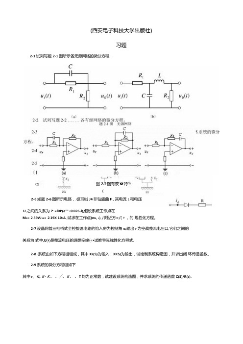
(西安电子科技大学出版社)习题2-1试列写题2-1图所示各无源网络的微分方程.M 0= 2.39VJ 11= 2.19X 10∙A ,试求在工作点(w 0, i 0}附近方=/(〃,的 规性化方程。
2-7设晶网管三相桥式全控整漉电路的怆入房为控制角α,输出r 为空战整流电压口,它们之间的 关系为 式中,U ⑷是整流电压的理想空竣(«•试推导其线性化方程式.2-8 ∙系统由如下方程祖组成,其中Xr(S)为输入,XKS)为输出,试绘制系统构造图,并求出闭 环传递函数。
2-9系统的微分方程组如下其中r 、K l . K- K 、、/、K 、、T 均为正常数,试建设系统构造图,并求系统的传递函数C(S)/R(s).图2-2图有双M 冷 ⑵(W <»U.之间的关系为i* =l0P(e""∕0.026-l),假设系统工作点在 2-6如题2∙6图所示电路,.极耳啦J4非钻盛曲F ,其电流L 和电压2-10试化简即2-10图所示的系统构造图.并求传递函数C(S)11R(S), K(S) C(S)/ C(S) R(S) 筑书规图所材 Gl C(S) G,卡G 5佛与函数 国S) C(S) G) 5 “七; Hl 弟统 £(S) M(S)2-16零初 设某 2-17 g (t) = 7-5e 6f . 咫2∙ 15图求系统 的传速函数, 始条件下的输出响试求该系统的传递 2-18系统的 W'> I 控制系统构造t f 1*1 2-16 W 系统构造图 R(S) ΛU) 2-15 E(S) C (Λ I I - L_rτ∏J ∙13图 系统G:" r ,(5) E(S)凤 F) R ⑸M ⑸松) ⅛4和脉冲响应函数, 单位脉冲响应为。
自动控制原理(中英文对照李道根)习题3.题解
■SolutionsP3.1 The unit step response of a certain system is given by t t e e t c 21)(---+=, 0≥t (a) Determine the impulse response of the system.(b) Determine the transfer function )()(s R s C of the system.Solution:The impulse response is the differential of corresponding step response, i.e.t t e e t tt c t k 22)(d )(d )(--+-==δAs we know that the transfer function is the Laplace transform of corresponding impulse response, i.e.232422111]2)([)()(222++++=+++-=+-=--s s s s s s e e t L s R s C tt δP3.2Consider the system described by the block diagram shown in Fig. P3.2(a). Determinethe polarities of two feedbacks for each of the following step responses shown in Fig. P3.2(b), where “0” indicates that the feedback is open.Solution:In general we have(a) Block diagram.1.1.1.1.1(b) U nit-step resp onses(1)(2)(3)(4)(5)Figure P3.221020221)()(k k s k s k k s R s C ±±=Note that the characteristic polynomial is210202)(k k s k s s ±±=∆where the sign of s k 2is depended on the outer feedback and the sign of 21k k is depended on the inter feedback.Case (1).The response presents a sinusoidal. It means that the system has a pair of pure imaginary roots, i.e. the characteristic polynomial is in the form of 212)(k k s s +=∆. Obviously, the outlet feedback is “–”and the inner feedback is “0”.Case (2).The response presents a diverged oscillation.The system has a pair of complex conjugate roots with positive real parts, i.e. the characteristic polynomial is in the form of 2122)(k k s k s s +-=∆. Obviously, the outlet feedback is “+”and the inner feedback is “–”.Case (3).The response presents a converged oscillation. It means that the system has a pair of complex conjugate roots with negative real parts, i.e. the characteristic polynomial is in the form of 2122)(k k s k s s ++=∆. Obviously,both the outlet and inner feedbacks are “–”.Case (4).In fact this is a ramp response of a first-order system. Hence, the outlet feedback is “0”to produce a ramp signal and the inner feedback is “–”.Case (5).Considering that a parabolic function is the integral of a ramp function, both the outlet and inner feedbacks are “0”.P3.3Consider each of the following closed-loop transfer function. By considering the location of the poles on the complex plane, sketch the unit step response, explaining the results obtained.(a) 201220)(2++=s s s Φ,(b) 61166)(23+++=s s s s Φ(c) 224)(2++=s s s Φ,(d) )5)(52(5.12)(2+++=s s s s ΦSolution:(a) )10)(2(20201220)(2++=++=s s s s s ΦBy inspection, the characteristic roots are 2-, 10-. This is an overdamped second-order system. Therefore, considering that the closed-loop gain is 1=Φk , its unit step response can be sketched as shown.(b) )3)(2)(1(661166)(23+++=+++=s s s s s s s ΦBy inspection, the characteristic roots are 1-, 2-, 3-.Obviously, all three transient components are decayed exponential terms. Therefore, its unit step response, with a closed-loop gain 1=Φk , is sketched as shown..1.1(c) 1)1(4224)(22++=++=s s s s ΦThis is an underdamped second-order system, because its characteristic roots are j ±-1. Hence, transient component is a decayed sinusoid. Noting that the closed-loop gain is 2=Φk , the unit step response can be sketched as shown.(d) )5](21[(5.12)5)(52(5.12)(222++=+++=s s s s s s )+ΦBy inspection, the characteristic roots are 21j ±-, 5-. Since51.0-<<-, there is a pair of dominant poles,21j ±-, for this system. The unit step response, with a closed-loop gain 5.0=Φk , is sketched as shown.P3.4 The open-loop transfer function of a unity negative feedback system is)1(1)(+=s s s G Determine the rise time, peak time, percent overshoot and setting time (using a 5% setting criterion).Solution: Writing he closed-loop transfer function2222211)(nn n s s s s s ωςωωΦ++=++=we get 1=n ω, 5.0=ς. Since this is an underdamped second-order system with 5.0=ς, the system performance can be estimated as follows.Rising time .sec 42.25.0115.0arccos 1arccos 22≈-⋅-=--=πςωςπn r t Peak time .sec 62.35.011122≈-⋅=-=πςωπn p t Percent overshoot %3.16%100%100225.015.01≈⨯=⨯=--πςπςσe e p Setting time .sec 615.033=⨯=≈ns t ςω(using a 5% setting criterion)P3.5 A second-order system gives a unit step response shown in Fig. P3.5. Find the open-loop transfer function if the system is a unit negative-feedback system.Solution:By inspection we have%30%100113.1=⨯-=p σSolving the formula for calculating the overshoot,.1.1Figure P3.5.0.23.021==-ςπςσe p , we have 362.0ln ln 22≈+-=ppσπσςSince .sec 1=p t , solving the formula for calculating the peak time, 21ςωπ-=n p t , we getsec/7.33rad n =ωHence, the open-loop transfer function is)4.24(7.1135)2()(2+=+=s s s s s G n n ςωωP3.6A feedback system is shown in Fig. P3.6(a), and its unit step response curve is shown in Fig. P3.6(b). Determine the values of 1k , 2k ,and a .Solution:The transfer function between the input and output is given by2221)()(k as s k k s R s C ++=The system is stable and we have, from the response curve,21lim )(lim 122210==⋅++⋅=→∞→k sk as s k k s t c s t By inspection we have%9%10000.211.218.2=⨯-=p σSolving the formula for calculating the overshoot, 09.021==-ςπςσe p , we have608.0ln ln 22≈+-=ppσπσςSince .sec 8.0=p t , solving the formula for calculating the peak time, 21ςωπ-=n p t , we getsec/95.4rad n =ωThen, comparing the characteristic polynomial of the system with its standard form, we have.2.2(a)(b)Figure P3.622222n n s s k as s ωςω++=++5.2495.4222===n k ω02.695.4608.022=⨯⨯==n a ςωP3.7A unity negative feedback system has the open-loop transfer function)2()(k s s k s G +=(a) Determine the percent overshoot.(b) For what range of k the setting time less than 0.75 s (using a 5% setting criterion).Solution: (a)For the closed-loop transfer function we have222222)(nn n s s k s k s ks ωςωωΦ++=++=hence, by inspection,we getsec /rad k n =ω, 22=ςThe percent overshoot is%32.4%10021=⨯=-ςπςσe p (b) Since 9.022<=ς, letting.sec 75.025.033<⨯=≈kt ns ςω(using a 5% setting criterion)results in2275.06⎪⎪⎭⎫⎝⎛>k , i.e. 32>k P3.8For the servomechanism system shown in Fig. P3.8,determine the values of k and a that satisfy the following closed-loop system design requirements.(a) Maximum of 40% overshoot.(b) Peak time of 4s.Solution:For the closed-loop transfer function we have22222)(nn n s s k s k s ks ωςωωαΦ++=++=hence, by inspection, we getk n =2ω, αςωk n =2,and n n k ωςςωα22==Taking consideration of %40%10021=⨯=-ςπςσe p results in280.0=ς.In this case, to satisfy the requirement of peak time, 412=-=ςωπn p t , we haveFigure P3.8.sec /818.0rad n =ωHence, the values of k and a are determined as67.02==n k ω, 68.02==nωςαP3.9 The open-loop transfer function of a unity feedback system is)2()(+=s s k s G A step response is specified as:peak time s 1.1=p t , and percent overshoot %5=p σ.(a) Determine whether both specifications can be met simultaneously. (b) If the specifications cannot be met simultaneously, determine a compromise value for k so that the peak time and percent overshoot are relaxed the same percentage.Solution:Writing the closed-loop transfer function222222)(nn n s s k s s ks ωςωωΦ++=++=we get k n =ωand k 1=ς.(a) Assuming that the peak time is satisfiedsec1.1112=-=-=k t n p πςωπwe get 16.9=k . Then, we have 33.0=ςand%5%33%10021>=⨯=-ςπςσe p Obviously, these two specifications cannot be met simultaneously.(b) In order to reduce p σthe gain must be reduced. Choosing sec 2.221==p p t t results in04.31=k , 57.01=ς, %102%3.111=>=p p σσRechoosing sec 31.21.22==p p t t results in85.21=k , 59.01=ς, %10.51.2%0.101=<=p p σσLetting sec 255.205.23==p p t t results in941.23=k , 583.03=ς, %10.2505.2%5.103=≈=p p σσIn this way, a compromise value is obtained as941.2=k P3.10A control system is represented by the transfer function)13.04.0)(56.2(33.0)()(2+++=s s s s R s C Estimate the peak time, percent overshoot, and setting time (%5=∆), using the dominant pole method, if it is possible.Solution:Rewriting the transfer function as]3.0)2.0)[(56.2(33.0)()(22+++=s s s R s C we get the poles of the system: 3.02.021j s ±-=,, 56.23-=s . Then, 21,s can be considered as a pair of dominant poles, because )Re()Re(321s s <<,.Method 1. After reducing to a second-order system,the transfer function becomes13.04.013.0)()(2++=s s s R s C (Note: 1)()(lim 0==→s R s C k s Φ)which results in sec /36.0rad n =ωand 55.0=ς. The specifications can be determined assec 0.42112ςωπ-=n p t , %6.12%10021=⨯=-ςπςσe p sec 67.2011ln 12=⎪⎪⎪⎭⎫⎝⎛-=ς∆ςωn s t Method 2. Taking consideration of the effect of non-dominant pole on the transient components cause by the dominant poles, we havesec0.8411)(231=--∠-=ςωπn p s s t %6.13%10021313=⨯-=-ςπςσe s s s p sec 6.232ln 1313=⎪⎪⎭⎫⎝⎛-⋅=s s s t n s ∆ςωP3.11By means of the algebraic criteria, determine the stability of systems that have thefollowing characteristic equations.(a) 02092023=+++s s s (b) 025103234=++++s s s s (c) 021*******=+++++s s s s s Solution:(a) 02092023=+++s s s . All coefficients of the characteristic equation are positive. Using L-C criterion,1609120202>==D This system is stable.(b) 025103234=++++s s s s . All coefficients of the characteristic equation are positive. Using L-C criterion,15311002531103<-==D This system is unstable.(c) 021*******=+++++s s s s s . (It’s better to use Routh criterion for a higher-order system.)All coefficients of the characteristicequation are positive. Establish the Routh arrayas shown.There are two changes of sign in the first column, this system is unstable.P3.12The characteristic equations for certain systems are given below. In each case,determine the number of characteristic roots in the right-half s -plane and the number of pure imaginary roots.(a) 0233=+-s s (b) 0160161023=+++s s s (c) 04832241232345=+++++s s s s s (d) 0846322345=--+++s s s s s Solution:(a) 0233=+-s s . The Routh array shows that there are two changes of sign in the first column. So that there are two characteristic roots in the right-half s -plane.(b) 0160161023=+++s s s The 1s -row is an all-zero one and an auxiliary equation is made based on 2s -row162=+s Taking derivative with respect to s yields2=s The coefficient of this new equation is inserted in the1s row, and the Routh array is then completed. By inspection, there are no changes of sign in the firstcolumn, and the system has no characteristic roots in the right-half s -plane. The solution of the auxiliary are 4j s ±=, the system has a pair of pure imaginary roots.(c) 04832241232345=+++++s s s s s . The Routh array is established as follows.The 1s -row is an all-zero one and an auxiliary equation based on 2s -row is42=+s Taking derivative with respect to s yields2=s The coefficient of this new equation isinserted in the 1s row, and the Routh array is then completed. By inspection, there are no changes of sign in the first column, and the system has no characteristic roots in the right-half5s 1914s 21023s 402s 1021s -0.800s 23s 1-32s 0 0>⇒ε21s εε23--0s 23s 1162s 101⇒16016⇒1s 02⇒0s 165s 112324s 31⇒248⇒4861⇒3s 41⇒164⇒2s 41⇒164⇒1s 02⇒0s 4s -plane. The solution of the auxiliary are 2j s ±=, the system has a pair of pure imaginaryroots.(d) 0846322345=--+++s s s s s .The Routh array is established as follows.The 3s -row is an all-zero one and an auxiliary equationbased on 4s -row is04324=-+s s Taking derivative with respect to s yields643=+s s The coefficient of this new equation is inserted in the 3s row, and the Routh array is then completed. By inspection, the sign inthe first column is changed one time, and the system has one root in the right-half s -plane. The solution of the auxiliary are 121±=,s 243j s ±=,, the system has one pair of pure imaginary roots.P3.13The characteristic equations for certain systems are given below. In each case, determine the value of k so that the corresponding system is stable. It is assumed that k is positive number.(a) 02102234=++++k s s s s (b) 0504)5.0(23=++++ks s k s Solution: (a) 02102234=++++k s s s s .The system is stable if and only if⎪⎪⎩⎪⎪⎨⎧<⇒>=>9022*********k k D k i.e. the system is stable when 90<<k .(b) 0504)5.0(23=++++ks s k s . The system is stable if and only if⎪⎩⎪⎨⎧>-+⇒>-+⇒>+=>>+0)3.3)(8.34(05024041505.00,05.022k k k k k k D k k i.e. the system is stable when 3.3>k .P3.14The open-loop transfer function of a negative feedback system is given by)12.001.0()(2++=s s s Ks G ςDetermine the range of K and ςin which the closed-loop system is stable.Solution: The characteristic equation is2.001.023=+++K s s s ςThe system is stable if and only if5s 13-44s 21⇒63⇒-84-⇒3s 04⇒06⇒02s 3-8 1s 5000s -8⎪⎩⎪⎨⎧<⇒>-⇒>=>>ςςς200010200101.02.002.0,02K K .ς.K D k The required range is 020>>K ς.P3.15The open-loop transfer function of negative feedback system is given)12)(1()1()()(+++=s Ts s s K s H s G The parameters K and T may be represented in a plane with K as the horizontal axis and T as the vertical axis. Determine the region in which the closed-loop system is stable.Solution:The characteristic equation is)1()2(223=+++++K s K s T Ts Since all coefficients are positive, the system is stable if and only if)1)(2(01222>++⇒>++=K T K T KT D 022>++-T KT K 04)2()2(>+-+-T T K 4)1)(2(<--⇒K T The system is stable in the region 4)1)(2(<--K T , which is plotted as shown. (Letting 2-='T T and 1-='K K results in 4<''K T .)P3.16A unity negative feedback system has an open-loop transfer function)1)(1)(1()(2+++=Ts n nTs Ts Ks G where 10≤≤n , 0>K , T is a positive constant.(a) Determine the range of K and n so that the system is stable.(b) Determine the value of K required for stability for 1=n , 0.5, 0.1, 0.01, and 0.(c) Discuss the stability of the closed-loop system as a function of n for a constant K .Solution:The closed-loop characteristic equation is)1)(1)(1(2=+++K Ts n nTs Ts +i.e. 01)1()(22223333=+++++++K Ts n n s T n n n s T n +(a) The system is stable if and only if)1(1)1(233222>+++++=Tn n Tn K T n n n D i.e.)1(0)1()1(2223322>--++⇒>+-++K n n n n T K T n n n ⎪⎪⎭⎫⎝⎛-++⎪⎪⎭⎫ ⎝⎛+++<⇒-⎪⎪⎭⎫⎝⎛++<1111112222n n n n n n K n n n K ⎪⎭⎫ ⎝⎛++<⇒⎪⎪⎭⎫⎝⎛-+++++<2222211)1(11)1(n n K n n n n n n n K '21hence, the system is stable when ⎪⎭⎫ ⎝⎛++<<2211)1(0n n K .(b) The value of K required for stability for 1=n , 0.5, 0.1, 0.01, and 0are calculated as shown.80<<K for 1=n ,5.110<<K for 5.0=n ,21.1220<<K for 1.0=n ,102020<<K for 01.0=n ,∞<<K 0for 0=n .(c) For a constant K , the stability of the closed-loop system is related to the value of n , the larger the value of n ,the easier the system to be stable. (Stagger principle.)P3.17A unity negative feedback system has an open-loop transfer function)16)(13()(++=s s s Ks G Determine the range of k required so that there are no closed-loop poles to the right of the line 1-=s .Solution:The closed-loop characteristic equation is18)6)(3(0)16)(13(=+++⇒=+++K s s s K ss s i.e. 01818923=+++K s s s Letting 1~-=s s resulting in)1018(~3~6~018)5~)(2~)(1~(23=-+++⇒=+++-K s s s K s s s Using Lienard-Chipart criterion, all closed-loop poles locate in the right-half s ~-plane, i.e. to the right of the line 1-=s , if and only if⎪⎩⎪⎨⎧<⇒>-⇒>-=>⇒>-91408.1820311018695,010182K K K D K K The required range is 91495<<K , or 56.10.56<<K P3.18A system has the characteristic equation291023=+++k s s s Determine the value of k so that the real part of complex roots is 2-, using the algebraiccriterion.Solution:Substituting 2~-=s s into the characteristic equation yields02~292~102~23=+-+-+-k s s s )()()(0)26(~~4~23=-+++k s s s The Routh array is established as shown.If there is a pair of complex roots with real part of 2-, then26=-k 3s 112s 426-k 1s 0si.e. 30=k . In the case of 30=k , we have the solution of the auxiliary equation j s ±=~, i.e. j s ±-=2.P3.19 An automatically guided vehicle is represented by the system in Fig. P3.19.(a) Determine the value of τrequired forstability.(b) Determine the value of τwhen one root of the characteristic equation is 5-=s , and the values of the remainingroots for the selected τ.(c) Find theresponse of the system to a step command for the τselected in (b).Solution:The closed-loop transfer function is10101010)()()(23+++==s s s s R s C s τΦ(a) The closed-loop characteristic equation is 010101023=+++s s s τSince all coefficients are positive, the system is stable if and only if1.0010110102>⇒>=ττD (b) Substituting 5~-=s s into the characteristic equation yields0105~105~105~23=+-+-+-)()()(s s s τ0)50135(~)2510(~5~23=-+-+-ττs s s In the case of 050135=-τ, i.e. 7.2=τ, we have 0~1=s , i.e. 51-=s . Solving the characteristic equation with 7.2=τ, i.e. 0~2~5~23=++-s s s results in 56.4~2=s and 44.0~3=s . Hence the remaining roots are 44.02-=s and 56.43-=s .(c) The closed-loop transfer function for 7.2=τis)5)(56.4)(44.0(10)(+++=s s s s ΦThe unit step response of the system is500.156.421.144.021.111)5)(56.4)(44.0(10)(+--+++-=⋅+++=s s s s s s s s s C tt t e e e t c 556.444.000.121.121.11)(----+-=Or, considering that there is a dominant pole for the system, we have127.2144.044.0)(+=+≈s s s Φte t c 44.01)(--≈P3.20A thermometer is described by the transfer function )11+Ts . It is known that, measuring the water temperature in a container, one minute is required to indicate 98% of the actual water temperature. Evaluate the steady-state indicating error of the thermometer if the container is heated and the water temperature is lineally increased at the rate of C/min 10 .travelFig.P3.19Solution:One minute required to indicate 98% of the actual water temperature means that the setting time is sec 604=≈T t s , i.e. the time constant of the thermometer issec15≈T The indicated error caused by the given ramp input, C/sec)(6010C/min)(10)( ==t t r , is222611611161)()()(sTs Ts s Ts s s C s R s E ⋅+=⋅+-=-=By inspection, a first-order system is always stable. Hence, the steady-state indicating error isC ss s s e s ss 5.26111515lim 20=⋅+⋅=→P3.21 Determine the steady-state error for a unit step input, a unit ramp input, and an acceleration input 22t for the following unit negative feedback systems. The open-loop transfer functions are given by(a) )12)(11.0(50)(++=s s s G ,(b) )5.0)(4(10)()(++=s s s s H s G (c) )11.0()15.0(8)(2++=s s s s G ,(d) )5)(1(10)(2++=s s s s G (e) )2004()(2++=s s s k s G Solution:(a) )12)(11.0(50)(++=s s s G . This is a second-order system and must be stable. Asa 0-type system,0=υ, the corresponding error constants are50=p K , 0=v K , 0=a K Consequently, the corresponding steady-state errors are0196.0501110.=+=+=p r ss K r ε, ∞==v v ss K v 0.ε, ∞==aa a ss K v .εrespectively.(b) )5.0)(4(10)()(++=s s s s H s G . The characteristic polynomial is40209)(23+++=s s s s τ∆Using L-C criterion,01402014092>==D the closed-loop system is stable. By inspection, system type 1=υand open-loop gain 5=K . Hence, the corresponding steady-state errors are0.=r ss ε, 2.01.==Kv ss ε, ∞=a ss .εrespectively.(c) )11.0()15.0(8)(2++=s s s s G . The characteristic polynomial is40209)(23+++=s s s s τ∆Using L-C criterion01402014092>==D the closed-loop system is stable. By inspection, system type 1=υand open-loop gain 5=K . Hence, the corresponding steady-state errors are0.=r ss ε, 2.01.==Kv ss ε, ∞=a ss .εrespectively.(d) )5)(1(10)(2++=s s s s G . The characteristic polynomial is1056)(234+++=s s s s ∆By inspection, this system is unstable (due to constructional instability).(e) )2004()(2++=s s s k s G . The characteristic polynomial isks s s s +++=2004)(23∆Using L-C criterionkkD -==800200142the closed-loop system is stable if and only if 8000<<k . This is a 1-type system with a open-loop gain 200k K =. In the case of 8000<<k , i.e. 40<<K ,the corresponding steady-state errors are0.=r ss ε, kK v ss 2001.==ε, ∞=a ss .εrespectively.P3.22 The open-loop transfer function of a unity negative feedback system is given by)1)(1()(21++=s T s T s Ks G Determine the values of K , 1T , and 2T so that the steady-state error for the input, bt a t r +=)(, is less than 0ε. It is assumed that K , 1T , and 2T are positive, a and b are constants.Solution:The characteristic polynomial is Ks s T T s T T s ++++=221321)()(∆Using L-C criterion, the system is stable if and only if2121212121212001T T T T K T KT T T T T K T T D +<⇒>-+⇒>+=Considering that this is a 1-type system with a open-loop gain K , in the case of 2121T T T T K +<, we have0..εεεεεbK Kbv ss r ss ss >⇒<=+=Hence, the required range for K is21210T T T T K b+<<εP3.23 The open-loop transfer function of a unity negative system is given by)1()(+=Ts s K s G Determine the values of K and T so that the following specifications are satisfied:(a) The steady-state error for the unit ramp input is less than 02.0.(b) The percent overshoot is less than %30and the setting time is less s 3.0.Solution:Assuming that both K and T are positive, the system must be stable. To meet the requirement on steady-state error, we have5002.010≥⇒≤==k KK v v ss εTo meet the second requirement, we have358.0%3021≥⇒≤=-ςσςπςe p and%)2(,10sec3.03=≥⇒≤≈∆ςωςωn ns t Considering that KT21=ςand TKn =ω, we get 95.1358.021≤⇒≥=KT KTς05.02010≤⇒=≥=T KT T K n ςωFinally, to met all specifications, the required ranges K and T are⎪⎩⎪⎨⎧≤≤≤T K T 95.15005.0P3.24 The block diagram of a control system is shown in Fig. P3.24, where)()()(s C s R s E -=. Select the values of τand b so that the steady-state error for a ramp input is zero.Figure P3.24Solution:Assuming that all parameters are positive, the system must be stable. Then, the error response is)()1)(1()(1)()()(21s R K s T s T b s K s C s R s E ⎥⎦⎤⎢⎣⎡++++-=-=τ)()1)(1()1()(2121221s R Ks T s T Kb s K T T s T T ⋅+++-+-++=τLetting the steady-state error for a ramp input to be zero, we get221212210.)1)(1()1()(lim )(lim sv Ks T s T Kb s K T T s T T s s sE s s r ss ⋅+++-+-++⋅==→→τεwhich results in⎩⎨⎧=-+=-00121τK T T Kb I.e. K T T 21+=τ, Kb 1=.P3.25 The block diagram of a compound system is shown in Fig. P3.25.Select the values ofa andb so that the steady-state error for a parabolic input is zero.Solution: The characteristic polynomial is 1012.0002.0)(23+++=s s s s ∆Using L-C criterion,1.01002.01012.02>==D the system is stable. The transfer function between error and input is given by10)102.0)(11.0()(10)102.0)(11.0()102.0)(11.0(101)102.0)(11.0()(101)()()(22++++-++=++++++-=-=s s s bs as s s s s s s s s s bs as s C s R s E 10)102.0)(11.0()101()101.0(002.023+++-+-+=s s s s b s a s Letting the steady-state error for a parabolic input to be zero yields010)102.0)(11.0()101()101.0(002.0lim 30230.=⋅+++-+-+⋅=→sa s s s sb s a s s s ass εwhich results inFigure P3.25⎩⎨⎧=-=-01012.00101a b i.e. 012.0=a , 1.0=b .P3.26 The block diagram of a system is shown in Fig. P3.26. In each case, determine the steady-state error for a unit step disturbance and a unit ramp disturbance, respectively.(a) 11)(K s G =, )1()(222+=s T s K s G (b) ss T K s G )1()(111+=, )1()(222+=s T s K s G , 21T T >Solution: (a) In this case the system is of second-order and must be stable. The transferfunction from disturbance to error is given by212212.)1(1)(K K Ts s K G G G s d e ++-=+-=ΦThe corresponding steady-state errors are12120.11)1(lim K s K K Ts s K s s p ss -=⋅++-⋅=→ε∞→⋅++-⋅=→22120.1)1(lim sK K Ts s K s s a ss ε(b) Now, the transfer function from disturbance to error is given by)1()1()(121222.+++-=s T K K s T s sK s d e Φand the characteristic polynomial is21121232)(K K s T K K s s T s +++=∆Using L-C criterion,)(121211212212>-==T T K K T K K T K K D the system is stable. The corresponding steady-state errors are01)1()1(lim 1212220.=⋅+++-⋅=→s s T K K s T s sK s s p ss ε121212220.11)1()1(lim K s s T K K s T s sK s s a ss -=⋅+++-⋅=→εFigure P3.26P3.27 The block diagram of a compound system is shown in Fig. P3.26, where1)(111+=s T K s G , )1()(222+=s T s K s G ,233)(K K s G =Determine the feedforward block transfer function )(s G d so that the steady-state error due tounit step disturbance is zero.Solution: the characteristic equation is 0121=+G G , i.e.21221321)(K K s s T T s T T ++++Using L-C criterion, the system is stable if and only if002121212121212>-+=+=T T K K T T T T K K T T D hence, the system is stable if212121T T T T K K +<The transfer function from disturbance to error is given by111)(1)1(1)(2211112322212123.+⋅++⎥⎦⎤⎢⎣⎡⋅+++-=+--=s T K s T K s G s T K K K s T s K G G G G G G G s dd de Φ21212113)1)(1()()1(K K s T s T s s G K K s T K d +++++-=When the system is stable, letting the steady-state error to be zero yields0)1)(1()()1(lim 0212121130=⋅⎥⎦⎤⎢⎣⎡+++++-⋅=→s d K K s T s T s s G K K s T K s d s ss ε[]0)()1(lim 21130=++→s G K K s T K d s i.e.213)(K K K s G d -=The feedforward block function is 213)(K K K s G d -=, where 212121T T TT K K +<.Figure P3.27。
自动控制原理习题及解答
dt 2
dt
(2-1)
此方程为二阶非线性齐次方程。
(5)线性化
由前可知,在θ =0 的附近,非线性函数 sinθ ≈θ ,故代入式(2-1)可得线
性化方程为
ml d 2θ + al dθ + mgθ = 0
dt 2
dt
例 2-3 已知机械旋转系统如图 2-3 所示,试列出系统运动方程。
图 2-3 机械旋转系统
U (s) = Z(s) I (s)
如果二端元件是电阻 R、电容 C 或电感 L,则复阻抗 Z(s)分别是 R、1/C s 或 L s。
(2) 用复阻抗写电路方程式:
I1
(S)
=
[U
r
(S
)
−
U
C1
(S )]
⋅
1 R1
U
c1
(S)
=
[I1(S
)
−
I
2
(S )]
⋅
1 C1s
I
2
(S
)
=
[U
c1
(S)
=1−
(L1
+
L2
+
L3 )
−
L1 L2
=1+
1 R1C1S
+
1 R2C2 S
+
1 R2 C1 S
(2-2)
式中,J 为摆杆围绕重心 A 的转动惯量。
摆杆重心 A 沿 X 轴方向运动方程为:
m d 2xA = H dt 2
即
m d 2 (x + l sinθ ) = H
(2
dt 2
-3)
摆杆重心 A 沿 y 轴方向运动方程为:
自控原理习题解答
②R(s)和N(s)同时作用时系统的输出
∴ C(s) = CR (s) + CN (s)
=
G1G2 + G1G3 + G1G2G3H1
R(s) +
1+ G1G3 + G2H1 + G1G2 + G1G2G3H1
+ 1+ G2H1 + G1G2G4 + G1G3G4 + G1G2G3G4H1 N (s) 1+ G1G3 + G2H1 + G1G2 + G1G2G3H1
s(s + 1)
Kts
1.试分析速度反馈系数Kt对系统稳定性的影响。 2.试求KP、Kv、Ka并说明内反馈对稳态误差的影响。 解: 1.如果没有内反馈,系统的开环和闭环传递函数为
解:将系统开环传递函数与二阶系统典型开环传递函
数比较: 所以:
G(s) =
ωn2
s(s + 2ζωn )
ωn = 10K
2ζωn = 10 ζωn = 5
ζ= 5
10K
−πζ
σ = e 1−ζ 2 ×100%
tp
=π ωd
=
ωn
π 1−ζ 2
tS
(5%)
≈
3
ζωn
分别将K=10 ,K=20代入计算,结果如下:
10K1 = 10 1 + 10 K 2
解之得:K2=0.9 K1=10
Ø 3-4 单位反馈系统的开环传递函数为
G(s) = K = 10K s(0.1s + 1) s(s +10)
试分别求出K=10s–1和K=20s–1时,系统的阻尼比ζ 和
自动控制原理英文版课后全部_答案
Module3Problem 3.1(a) When the input variable is the force F. The input variable F and the output variable y are related by the equation obtained by equating the moment on the stick:2.233y dylF lk c l dt=+Taking Laplace transforms, assuming initial conditions to be zero,433k F Y csY =+leading to the transfer function31(4)Y k F c k s=+ where the time constant τ is given by4c kτ=(b) When F = 0The input variable is x, the displacement of the top point of the upper spring. The input variable x and the output variable y are related by the equation obtained by the moment on the stick:2().2333y y dy k x l kl c l dt-=+Taking Laplace transforms, assuming initial conditions to be zero,3(24)kX k cs Y =+leading to the transfer function321(2)Y X c k s=+ where the time constant τ is given by2c kτ=Problem 3.2 P 54Determine the output of the open-loop systemG(s) = 1asT+to the inputr(t) = tSketch both input and output as functions of time, and determine the steady-state error between the input and output. Compare the result with that given by Fig3.7 . Solution :While the input r(t) = t , use Laplace transforms, Input r(s)=21sOutput c(s) = r(s) G(s) = 2(1)aTs s ⋅+ = 211T T a s s Ts ⎛⎫ ⎪-+ ⎪ ⎪+⎝⎭the time-domain response becomes c(t) = ()1t Tat aT e ---Problem 3.33.3 The massless bar shown in Fig.P3.3 has been displaced a distance 0x and is subjected to a unit impulse δ in the direction shown. Find the response of the system for t>0 and sketch the result as a function of time. Confirm the steady-state response using the final-value theorem. Solution :The equation obtained by equating the force:00()kx cxt δ+=Taking Laplace transforms, assuming initial condition to be zero,K 0X +Cs 0X =1leading to the transfer function()XF s =1K Cs +=1C1K s C+The time-domain response becomesx(t)=1CC tK e -The steady-state response using the final-value theorem:lim ()t x t →∞=0lim s →s 1K Cs +1s =1K00000()()()1;11111()K t CK x x Cx t Kx X K Cs Kx Kx X C Cs K K s KKx x t eCδ-++=⇒++=--∴==⋅++-=⋅According to the final-value theorem:0001lim ()lim lim 01t s s Kx sx t s X C K s K→∞→→-=⋅=⋅=+ Problem 3.4 Solution:1.If the input is a unit step, then1()R s s=()()11R s C s sτ−−−→−−−→+ leading to,1()(1)C s s sτ=+taking the inverse Laplace transform gives,()1tc t e τ-=-as the steady-state output is said to have been achieved once it is within 1% of the final value, we can solute ―t‖ like this,()199%1tc t e τ-=-=⨯ (the final value is 1) hence,0.014.60546.05te t sττ-==⨯=(the time constant τ=10s)2.the numerical value of the numerator of the transfer function doesn’t affect the answer. See this equation, If ()()()1C s AG s R s sτ==+ then()(1)A C s s sτ=+giving the time-domain response()(1)tc t A e τ-=-as the final value is A, the steady-state output is achieved when,()(1)99%tc t A e A τ-=-=⨯solute the equation, t=4.605τ=46.05sthe result make no different from that above, so we said that the numerical value of the numerator of the transfer function doesn’t affect the answer.If a<1, as the time increase, the two lines won`t cross. In the steady state the output lags the input by a time by more than the time constant T. The steady error will be negative infinite.R(t)C(t)Fig 3.7 tR(t)C(t)tIf a=1, as the time increase, the two lines will be parallel. It is as same as Fig 3.7.R(t)C(t)tIf a>1, as the time increase, the two lines will cross. In the steady state the output lags the input by a time by less than the time constant T.The steady error will be positive infinite.Problem 3.5 Solution: R(s)=261s s+, Y(s)=26(51)s s s +⋅+=229614551s s s -+++ /5()62929t y t t e -∴=-+so the steady-state error is 29(-30). To conform the result:5lim ()lim(62929);tt t y t t -→∞→∞=-+=∞6lim ()lim ()lim ()lim(51)t s s s s y t y s Y s s s →∞→→→+====∞+.20lim ()lim ()lim [()()]161lim [()1]()lim (1)()5130ss t s s s s e e t S E S S Y S R S S G S R S S S S S→∞→→→→==⋅=⋅-=⋅-=⋅-⋅++=- Therefore, the solution is basically correct.Problem 3.623yy x += since input is of constant amplitude and variable frequency , it can be represented as:j tX eA ω=as we know ,the output should be a sinusoidal signal with the same frequency of the input ,it can also be represented as:R(t)C(t)t0j t y y e ω=hence23j tj tj tj yyeeeA ωωωω+=00132j y Aω=+ 0294Ayω=+ 2tan3w ϕ=- Its DC(w→0) value is 003Ay ω==Requirement 01122w yy==21123294AA ω=⨯+ →32w = while phase lag of the input:1tan 14πϕ-=-=-Problem 3.7One definition of the bandwidth of a system is the frequency range over which the amplitude of the output signal is greater than 70% of the input signal amplitude when a system is subjected to a harmonic input. Find a relationship between the bandwidth and the time constant of a first-order system. What is the phase angle at the bandwidth frequency ? Solution :From the equation 3.41000.71r A r ωτ22=≥+ (1)and ω≥0 (2) so 1.020ωτ≤≤so the bandwidth 1.02B ωτ=from the equation 3.43the phase angle 110tan tan 1.024c πωτ--∠=-=-=Problem 3.8 3.8 SolutionAccording to generalized transfer function of First-Order Feedback Systems11C KG K RKGHK sτ==+++the steady state of the output of this system is 2.5V .∴if s →0, 2.51104C R→=. From this ,we can get the value of K, that is 13K =.Since we know that the step input is 10V , taking Laplace transforms,the input is 10S.Then the output is followed1103()113C s S s τ=⨯++Taking reverse Laplace transforms,4/4332.5 2.5 2.5(1)t t C e eττ--=-=-From the figure, we can see that when the time reached 3s,the value of output is 86% of the steady state. So we can know34823(2)*4393τττ-=-⇒-=-⇒=, 4/3310.8642t t e ττ-=-=⇒=The transfer function is3128s +146s+Let 12+8s=0, we can get the pole, that is 1.5s =-2/3- Problem 3.9 Page 55 Solution:The transfer function can be represented,()()()()()()()o o m i m i v s v s v s G s v s v s v s ==⋅While,()1()111//()()11//o m m i v s v s sRCR v s sC sC v s R R sC sC =+⎛⎫+ ⎪⎝⎭=⎡⎤⎛⎫++ ⎪⎢⎥⎝⎭⎣⎦Leading to the final transfer function,21()13()G s sRC sRC =++ And the reason:the second simple lag compensation network can be regarded as the load of the first one, and according to Load Effect , the load affects the primary relationship; so the transfer function of the comb ination doesn’t equal the product of the two individual lag transfer functio nModule4Problem4.14.1The closed-loop transfer function is10(6)102(6)101610S S S S C RS s +++++==Comparing with the generalized second-order system,we getProblem4.34.3Considering the spring rise x and the mass rise y. Using Newton ’s second law of motion..()()d x y m y K x y c dt-=-+Taking Laplace transforms, assuming zero initial conditions2mYs KX KY csX csY =-+-resulting in the transfer funcition where2Y cs K X ms cs K +=++ And521.26*10cmkc ζ== Problem4.4 Solution:The closed-loop transfer function is210263101011n n d n W EW E W W E ====-=2121212K C K S S K R S S K S S ∙+==+++∙+Comparing the closed-loop transfer function with the generalized form,2222n n nCR s s ωξωω=++ it is seen that2n K ω= And that22n ξω= ; 1Kξ=The percentage overshoot is therefore21100PO eξπξ--=11100k keπ-∙-=Where 10%PO ≤When solved, gives 1.2K ≤(2.86)When K takes the value 1.2, the poles of the system are given by22 1.20s s ++=Which gives10.45s j =-±±s=-1 1.36jProblem4.5ReIm0.45-0.45-14.5 A unity-feedback control system has the forward-path transfer functionG (s) =10)S(s K+Find the closed-loop transfer function, and develop expressions for the damping ratio And damped natural frequency in term of K Plot the closed-loop poles on the complex Plane for K = 0,10,25,50,100.For each value of K calculate the corresponding damping ratio and damped natural frequency. What conclusions can you draw from the plot?Solution: Substitute G(s)=(10)K s s + into the feedback formula : Φ(s)=()1()G S HG S +.And in unitfeedback system H=1. Result in: Φ(s)=210Ks s K++ So the damped natural frequencyn ω=K ,damping ratio ζ=102k =5k.The characteristic equation is 2s +10S+K=0. When K ≤25,s=525K -±-; While K>25,s=525i K -±-; The value ofn ω and ζ corresponding to K are listed as follows.K 0 10 25 50 100 Pole 1 1S 0 515-+ -5 -5+5i 553i -+Pole 2 2S -10 515-- -5 -5-5i553i --n ω 010 5 52 10 ζ ∞2.51 0.5 0.5Plot the complex plane for each value of K:We can conclude from the plot.When k ≤25,poles distribute on the real axis. The smaller value of K is, the farther poles is away from point –5. The larger value of K is, the nearer poles is away from point –5.When k>25,poles distribute away from the real axis. The smaller value of K is, the further (nearer) poles is away from point –5. The larger value of K is, the nearer (farther) poles is away from point –5.And all the poles distribute on a line parallels imaginary axis, intersect real axis on the pole –5.Problem4.61tb b R L C b o v dv i i i i v dt C R L dt=++=++⎰Taking Laplace transforms, assuming zero initial conditions, reduces this equation to011b I Cs V R Ls ⎛⎫=++ ⎪⎝⎭20b V RLs I Ls R RLCs =++ Since the input is a constant current i 0, so01I s=then,()2b RLC s V Ls R RLCs==++ Applying the final-value theorem yields ()()0lim lim 0t s c t sC s →∞→==indicating that the steady-state voltage across the capacitor C eventually reaches the zero ,resulting in full error.Problem4.74.7 Prove that for an underdamped second-order system subject to a step input, thepercentage overshoot above the steady-state output is a function only of the damping ratio .Fig .4.7SolutionThe output can be given by222222()(2)21()(1)n n n n n n C s s s s s s s ωζωωζωζωωζ=+++=-++- (1)the damped natural frequencyd ω can be defined asd ω=21n ωζ- (2)substituting above results in22221()()()n n n d n d s C s s s s ζωζωζωωζωω+=--++++ (3) taking the inverse transform yields22()1sin()11tan n t d e c t t where ζωωφζζφζ-=-+--=(4)the maximum output is22()1sin()11n t p d p p d n e c t t t ζωωφζππωωζ-=-+-==-(5)so the maximum is2/1()1p c t eπζζ--=+the percentage overshoot is therefore2/1100PO eπζζ--=Problem4.8 Solution to 4.8:Considering the mass m displaced a distance x from its equilibrium position, the free-body diagram of the mass will be as shown as follows.aP cdx kxkxmUsing Newton ’s second law of motion,22p k x c x mx m x c x k x p--=++=Taking Laplace transforms, assuming zero initial conditions,2(2)X ms cs k P ++= results in the transfer function2/(1/)/((/)2/)X P m s c m s k m =++ 2(2/)(2/)((/)2/)k k m s c m s k m =++As we see2(2)X m s c s k P++= As P is constantSo X ∝212ms cs k ++ . When 56.25102cs m-=-=-⨯ ()25min210mscs k ++=4max5100.110X == This is a second-order transfer function where 22/n k m ω= and/2/22n c w m c k m ζ== The damped natural frequency is given by 2212/1/8d n k m c km ωωζ=-=-22/(/2)k m c m =- Using the given data,462510/2100.050.2236n ω=⨯⨯⨯== 462502.79501022100.05ζ-==⨯⨯⨯⨯ ()240.22361 2.7950100.2236d ω-=⨯-⨯= With these data we can draw a picture14.0501160004.673600p de s e T T πωτζωτ======222222112/1222()22,,,428sin (sin cos )0tan 7.030.02n n pp dd n dd n ntd d t t t n d p d d p ddd p p p nX k m c k P ms cs k k m s s s m m k c k c cm m m m km p x e tm p xe t t m t t x m ζωζωωωζωωωωζζωωωζωωωωωωωζω--===⋅=⋅++++++=-===∴==-+=∴=⇒=⇒= 其中Problem4.10 4.10 solution:The system is similar to the one in the book on PAGE 58 to PAGE 63. The difference is the connection of the spring. So the transfer function is2222l n d n n w s w s w θθζ=++222(),;p a m ld a m p m l m l l m mm l lk k k N RJs RCs R k k N k J N J J C N c c N N N θθωθωθ=+++=+=+===p a mn K K K w NJ R='damping ratio 2p a m c NRK K K J ζ='But the value of J is different, because there is a spring connected.122s m J J J J N N '=++Because of final-value theorem,2l nd w θθζ=Module5Problem5.45.4 The closed-loop transfer function of the system may be written as2221010(1)610101*********CR K K K S S K K S S K S S +++==+++++++ The closed-loop poles are the solutions of the characteristic equation6364(1010)3110210(1)n K S K JW K -±-+==-±+=+ 210(1)6310(1)E K E K +==+In order to study the stability of the system, the behavior of the closed-loop poles when the gain K increases from zero to infinte will be observed. So when12K = 3010E =321S J =-± 210K = 3110110E =3101S J =-± 320K = 21070E =3201S J =-±双击下面可以看到原图ReProblem5.5SolutionThe closed-loop transfer function is2222(1)1(1)KC K KsKR s K as s aKs Kass===+++++∙+Comparing the closed-loop transfer function with the generalized form, 2222nn nCR s sωξωω=++Leading to2nKa Kωξ==The percentage overshoot is therefore2110040%PO eξπξ--==Producing the result0.869ξ=(0.28)And the peak time241PnT sπωξ==-Leading to1.586nω=(0.82)Problem5.75.7 Prove that the rise time T r of a second-order system with a unit step input is given byT r = d ω1 tan -1n dζωω = d ω1 tan -1d ωζ21--Plot the rise against the damping ratio.Solution:According to (4.33):c(t)=1-2(cos sin )1n t d d e t t ζωζωωζ-+-. 4.33When t=r T ,c(t)=1.substitue c(t)= 1 into (4.33) Producing the resultr T =d ω1 tan -1n dζωω = d ω1 tan -112ζζ--Plot the rise time against the damping ratio:Problem5.9Solution to 5.9:As we know that the system is the open-loop transfer function of a unity-feedback control system.So ()()GH S G S = Given as()()()425KGH s s s =-+The close-loop transfer function of the system may be written as()()()()()41254G s C Ks R GH s s s K ==+-++ The characteristic equation is()()2254034100s s K s s K -++=⇒++-=According to the Routh ’s method, the Routh ’s array must be formed as follow20141030410s K s s K -- For there is no closed-loop poles to the right of the imaginary axis4100 2.5K K -≥⇒≥ Given that 0.5ζ=4103 4.752410n K K K ωζ=-=⇒=- When K=0, the root are s=+2,-5According to the characteristic equation, the solutions are349424s K =-±-while 3.0625K ≤, we have one or two solutions, all are integral number.Or we will have solutions with imaginary number. So we can drawK=102 -5 K=0K=3.0625K=2.5 K=10Open-loop polesClosed-loop polesProblem5.10 5.10 solution:0.62/n w rad sζ==according to()211sin()21n w t d e c w t ζφζ-=-+=- 1.2sin(1.6)0.4t e t φ-⋅+= 4t a n3φ= finally, t is delay time:1.23t s ≈(0.67)Module6Problem 6.3First we assume the disturbance D to be zero:e R C =-1011C K e s s =⋅⋅⋅+Hence:(1)10(1)e s s R K s s +=++ Then we set the input R to be zero:10()(1)C K e D e s s =⋅+⋅=-+ ⇒ 1010(1)e D K s s =-++Adding these two results together:(1)1010(1)10(1)s s e R D K s s K s s +=⋅-⋅++++21()R s s =; 1()D s s= ∴222110910(1)10(1)100(1)s s e Ks s s Ks s s s s s +-=-=++++++ the steady-state error:232200099lim lim lim 0.09100100ss s s s s s s e s e s s s s s →→→--=⋅===-++++Problem 6.4Determine the disturbance rejection ratio(DRR) for the system shown in Fig P.6.4+fig.P.6.4 solution :from the diagram we can know :0.210.05mv K RK c === so we can get that()0.21115()0.05v m m OL n CL K K DRR cR ωω∆⨯==+=+=∆210.10.050.050.025s s =++, so c=0.025, DRR=9Problem 6.5 6.5 SolutionFor the purposes of determining the steady-state error of the system, we should get to know the effect of the input and the disturbance along when the other will be assumed to be zero.First to simplify the block diagram to the following patter:110s +2021Js Tddθoθ0.220.10.05s ++__+d T—Allowing the transfer function from the input to the output position to be written as01220220d Js s θθ=++ 012222020240*220220(220)dJs s Js s s Js s sθθ===++++++ According to the equation E=R-C:022*******(2)()lim[()()]lim[(1)]lim 0.2220220ssr d s s s Js e s s s s Js s Js s δδδθθ→→→+=-=-==++++问题;1. 系统型为2,对于阶跃输入,稳态误差为0.2. 终值定理写的不对。
自动控制原理课后习题答案
第一章引论1-1 试描述自动控制系统基本组成,并比较开环控制系统和闭环控制系统的特点。
答:自动控制系统一般都是反馈控制系统,主要由控制装置、被控部分、测量元件组成。
控制装置是由具有一定职能的各种基本元件组成的,按其职能分,主要有给定元件、比较元件、校正元件和放大元件。
如下图所示为自动控制系统的基本组成。
开环控制系统是指控制器与被控对象之间只有顺向作用,而没有反向联系的控制过程。
此时,系统构成没有传感器对输出信号的检测部分。
开环控制的特点是:输出不影响输入,结构简单,通常容易实现;系统的精度与组成的元器件精度密切相关;系统的稳定性不是主要问题;系统的控制精度取决于系统事先的调整精度,对于工作过程中受到的扰动或特性参数的变化无法自动补偿。
闭环控制的特点是:输出影响输入,即通过传感器检测输出信号,然后将此信号与输入信号比较,再将其偏差送入控制器,所以能削弱或抑制干扰;可由低精度元件组成高精度系统。
闭环系统与开环系统比较的关键,是在于其结构有无反馈环节。
1-2 请说明自动控制系统的基本性能要求。
答:、自动控制系统的基本要求概括来讲,就是要求系统具有稳定性、快速性和准确性。
稳定性是对系统的基本要求,不稳定的系统不能实现预定任务。
稳定性通常由系统的结构决定与外界因素无关。
对恒值系统,要求当系统受到扰动后,经过一定时间的调整能够回到原来的期望值(例如恒温控制系统)。
对随动系统,被控制量始终跟踪参量的变化(例如炮轰飞机装置)。
快速性是对过渡过程的形式和快慢提出要求,因此快速性一般也称为动态特性。
在系统稳定的前提下,希望过渡过程进行得越快越好,但如果要求过渡过程时间很短,可能使动态误差过大,合理的设计应该兼顾这两方面的要求。
准确性用稳态误差来衡量。
在给定输入信号作用下,当系统达到稳态后,其实际输出与所期望的输出之差叫做给定稳态误差。
显然,这种误差越小,表示系统的精度越高,准确性越好。
当准确性与快速性有矛盾时,应兼顾这两方面的要求。
自动控制原理-课后习题及答案
第一章 绪论1-1 试比较开环控制系统和闭环控制系统的优缺点.解答:1开环系统(1) 优点:结构简单,成本低,工作稳定。
用于系统输入信号及扰动作用能预先知道时,可得到满意的效果。
(2) 缺点:不能自动调节被控量的偏差。
因此系统元器件参数变化,外来未知扰动存在时,控制精度差。
2 闭环系统⑴优点:不管由于干扰或由于系统本身结构参数变化所引起的被控量偏离给定值,都会产生控制作用去清除此偏差,所以控制精度较高。
它是一种按偏差调节的控制系统。
在实际中应用广泛。
⑵缺点:主要缺点是被控量可能出现波动,严重时系统无法工作。
>1-2 什么叫反馈为什么闭环控制系统常采用负反馈试举例说明之。
解答:将系统输出信号引回输入端并对系统产生控制作用的控制方式叫反馈。
闭环控制系统常采用负反馈。
由1-1中的描述的闭环系统的优点所证明。
例如,一个温度控制系统通过热电阻(或热电偶)检测出当前炉子的温度,再与温度值相比较,去控制加热系统,以达到设定值。
1-3 试判断下列微分方程所描述的系统属于何种类型(线性,非线性,定常,时变)(1)22()()()234()56()d y t dy t du t y t u t dt dt dt ++=+(2)()2()y t u t =+(3)()()2()4()dy t du t ty t u t dt dt +=+ (4)()2()()sin dy t y t u t tdt ω+=(5)22()()()2()3()d y t dy t y t y t u t dt dt ++=—(6)2()()2()dy t y t u t dt +=(7)()()2()35()du t y t u t u t dtdt =++⎰解答: (1)线性定常 (2)非线性定常 (3)线性时变(4)线性时变 (5)非线性定常 (6)非线性定常 (7)线性定常1-4 如图1-4是水位自动控制系统的示意图,图中Q1,Q2分别为进水流量和出水流量。
- 1、下载文档前请自行甄别文档内容的完整性,平台不提供额外的编辑、内容补充、找答案等附加服务。
- 2、"仅部分预览"的文档,不可在线预览部分如存在完整性等问题,可反馈申请退款(可完整预览的文档不适用该条件!)。
- 3、如文档侵犯您的权益,请联系客服反馈,我们会尽快为您处理(人工客服工作时间:9:00-18:30)。
(d) (s)
12.5
(s 2 2s 5)(s 5)
Solution: (a) (s)
■Solutions
■Solutions
P3.1 The unit step response of a certain system is given by c(t) 1 e t e2t , t 0
(a) Determine the impulse response of the system. (b) Determine the transfer function C(s) R(s) of the system.
R (s)
k1
s
0
k2
s
0
C (s )
(a) Block diagram
c (t)
c (t)
c(t)
1.0
1.0
1.0
t
t
t
0
0
0
(1)
(2)
(3)
c (t)
c(t) Asy mp totic
Parabolic
line
1.0
1.0
t 0
(4 )
t
0
(5 )
(b) Unit-step resp onses
response, i.e.
C(s) L[ (t) e t 2e2t ] 1 1 2 s 2 4s 2
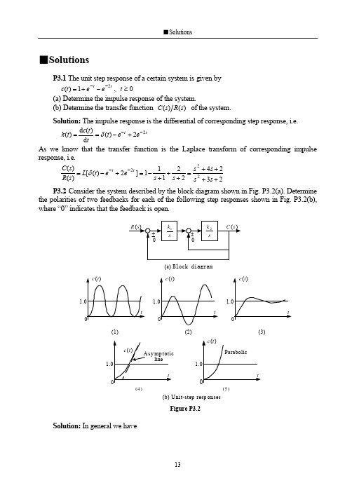
P3.2 Consider the system described by the block diagram shown in Fig. P3.2(a). Determine the polarities of two feedbacks for each of the following step responses shown in Fig. P3.2(b), where “0” indicates that the feedback is open.
location of the poles on the complex plane, sketch the unit step response, explaining the results
obtained.
(a)
(s)
s2
20 12s
20
,
(b)
(s)
s3
6 6s2 11s
6
(c) (s) 4 , s2 2s 2
Case (2). The response presents a diverged oscillation. The system has a pair of complex conjugate roots with positive real parts, i.e. the characteristic polynomial is in the form of (s) s 2 k2 s k1k2 . Obviously, the outlet feedback is “+” and the inner feedback is “–”.
Case (4). In fact this is a ramp response of a first-order system. Hence, the outlet feedback is “0” to produce a ramp signal and the inner feedback is “–”.
Case (3). The response presents a converged oscillation. It means that the system has a pair of complex conjugate roots with negative real parts, i.e. the characteristic polynomial is in the form of (s) s 2 k2 s k1k2 . Obviously, both the outlet and inner feedbacks are “–”.
Figure P3.2
Solution: In general we have
13
■Solutions
C(s)
k1 k 2
R(s)
s2
0
k
2
s
0
k1 k 2
Note that the characteristic polynomial is
(s)
s2
0
k2
s
0
k1 k 2
where the sign of k2 s is depended on the outer feedback and the sign of k1k2 is depended on
the inter feedback.
Case (1). The response presents a sinusoidal. It means that the system has a pair of pure imaginary roots, i.e. the characteristic polynomial is in the form of (s) s 2 k1k2 . Obviously, the outlet feedback is “–”and the inner feedback is “0”.
Solution: The impulse response is the differential of corresponding step response, i.e.
k(t) dc(t) (t) et 2e 2t dt
As we know that the transfer function is the Laplace transform of corresponding impulse
Case (5). Considering that a parabolic function is the integral of a ramp function, both the outlet and inner feedbacks are “0”.
P3.3 Consider each of the following closed-loop transfer function. By considering the