R语言 House Price 预测房价数据挖掘分析报告 附代码数据
房地产数据R语言分析

-Exclude the Order, PID, and of course SalesPrice variables from your predictors.在变量中要去除Order, PID, 当然SalesPrice也要去掉。
AmesHousing=AmesHousing[,-c(1,2 )]一个class是大于USD 200,000,另一类小于USD 20,000>=200000 :1<200000 :0AmesHousing$SalePrice <-ifelse(AmesHousing$SalePrice>200000,1,0)看看线性关系如何,如果不够好那么就要做变换(transformation)head(AmesHousing2)MS.SubClass Lot.Frontage Lot.Area Overall.Qual Overall.Cond Year.Bui lt1 20 141 31770 6 5 19 602 20 80 11622 5 6 19 613 20 81 14267 6 6 19 584 20 93 11160 75 19 685 60 74 13830 5 5 19 976 60 78 9978 6 6 19 98Year.Remod.Add Mas.Vnr.Area BsmtFin.SF.1 BsmtFin.SF.2 Bsmt.Unf.SF1 1960 112 639 0 4412 1961 0 468 144 2703 1958 108 923 0 4064 1968 0 1065 0 10455 1998 0 791 0 1376 1998 20 602 0 324Total.Bsmt.SF X1st.Flr.SF X2nd.Flr.SF Low.Qual.Fin.SF Gr.Liv.Area1 1080 1656 0 0 16562 882 896 0 0 8963 1329 1329 0 0 13294 2110 2110 0 0 21105 928 928 701 0 16296 926 926 678 0 1604Bsmt.Full.Bath Bsmt.Half.Bath Full.Bath Half.Bath Bedroom.AbvGr1 1 0 1 0 32 0 0 1 0 23 0 0 1 1 34 1 0 2 1 35 0 0 2 1 36 0 0 2 1 3Kitchen.AbvGr TotRms.AbvGrd Fireplaces Garage.Yr.Blt Garage.Cars1 1 72 1960 22 1 5 0 1961 13 1 6 0 1958 14 1 8 2 1968 25 16 1 1997 26 17 1 1998 2Garage.Area Wood.Deck.SF Open.Porch.SF Enclosed.Porch X3Ssn.Porch1 528 210 62 0 02 730 140 0 0 03 312 393 36 0 04 522 0 0 0 05 482 212 34 0 06 470 360 36 0 0Screen.Porch Pool.Area Misc.Val Mo.Sold Yr.Sold SalePrice1 0 0 0 5 2010 12 120 0 0 6 2010 03 0 0 12500 6 2010 04 0 0 0 4 2010 15 0 0 0 3 2010 06 0 0 0 6 2010 0有一些变量可能需要整合合并关键词"Flr","Porch","Bath","Overall","Sold",SF","Year","AbvGr","Garag e","Area"MS.SubClass Lot.Frontage Fireplaces Misc.Val SalePrice Flr Porch Ba th1 20 1412 0 1 1656 62 22 20 80 0 0 0 896 120 13 20 81 0 12500 0 1329 36 24 20 93 2 0 1 2110 0 45 60 74 1 0 0 1629 34 36 60 78 1 0 0 1604 36 3Overall Sold SF Year AbvGr Garage Area1 11 2015 2370 3920 11 2490 335382 11 2016 1904 3922 8 2692 125183 12 2016 3051 3916 10 2271 157044 12 2014 4220 3936 12 2492 132705 10 2013 2068 3995 10 2481 154596 12 2016 2212 3996 11 2470 11602plot(AmesHousing2)4.跑logistic regression, GAM, LDA, KNN这几个模型logistic regressionprint(paste('Accuracy',1-misClasificError))[1] "Accuracy 0.932166301969365"library("mgcv")gam建模misClasificError <-mean(fitted.results !=Ames.test$SalePrice,na.rm=T) print(paste('Accuracy',1-misClasificError))[1] "Accuracy 0.911062906724512"Knnlibrary(kknn)print(paste('Accuracy',1-misClasificError))[1] "Accuracy 0.585284280936455"LDAmisClasificError <-mean(fitted.results !=Ames.test$SalePrice,na.rm=T) print(paste('Accuracy',1-misClasificError))[1] "Accuracy 0.923413566739606"。
【原创】R语言数据挖掘统计预测模型课件教案讲义(附代码数据)

Class 8
Jeff Webb
Jeff Webb
IS 6489: Statistics and Predictive Analytics
1 / report expectations Homework discussion Class 8 topics:
Jeff Webb
IS 6489: Statistics and Predictive Analytics
7 / 51
Logistic regression: the model
The logistic regression model can be written in terms of log odds: log Pr(yi = 1|xi ) Pr(yi = 0|xi ) = Xi β
2 / 51
Final Report Expectations
Jeff Webb
IS 6489: Statistics and Predictive Analytics
3 / 51
Final report
PDF of the project assignment is available at Canvas Length: 5 pages of text plus additional pages, if necessary, for relevant plots and tables. Expectation: a client-ready report using best practices of technical writing and statistical communication, using graphs when possible, labeling and explaining them, and interpreting statistical results using language and quantities that non-statisticians can understand. Elements:
R语言房价回归预测案例报告 附代码数据
【原创】R语言报告论文(附代码数据)
有问题到淘宝找“大数据部落”就可以了
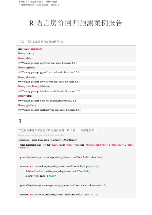
R语言房价回归预测案例报告首先,我们加载数据和必要的软件包:
1
1.
上面绘制的房屋年龄分布是非常正确的。
2.我们看到三个峰值,表明分布是多模态的。
这个数据集中的大部分房子(约140个)都是
10-15岁。
第二类房屋(约80人)年龄在55-60岁之间,分布右边的第三类房屋(约37户)的年龄在90-95岁之间。
这可能表示指定期间房地产业务的繁荣。
3.分配表明,超过45%的房屋建于不到45年前。
2
【原创】R语言报告论文(附代码数据)
有问题到淘宝找“大数据部落”就可以了
##计算由邻居分组并存储在数据框中的所有中央和传播统计数据。
ames_stats<-ames_train%>%group_by(Neighborhood)%>%summarise(Min=min(price, na.rm=TRUE), Mean=me。
用R语言进行数据挖掘与分析

用R语言进行数据挖掘与分析
一、前言
数据挖掘和分析是当今社会中非常重要的研究方向,因为大量的数据产生和存储已经成为我们的日常,而如何从这些数据中获取有益信息和规律是非常重要的。
而R语言作为数据科学领域中最重要的编程语言之一,受到了广泛的认可,并在越来越多的领域中应用起来。
本文就用R语言来进行数据挖掘和分析。
二、数据的获取
数据的获取是进行数据分析和挖掘的第一步。
这里我们选择了一个房价数据集来进行分析。
数据集包括了所统计城市的房屋信息、售价、建筑面积、交通情况、商业情况、房间数量和面积等信息。
我们可以使用R语言中的read.csv函数读取该csv格式的数据集,并将其存储在一个变量中。
```
house_data <- read.csv(\。
r语言 去除极值并统计

r语言去除极值并统计R语言是一种用于数据分析和统计的编程语言。
在进行数据分析时,经常需要处理极值(outliers),即远离其他数据点的异常值。
去除极值可以帮助我们更准确地分析数据,避免异常值对结果的影响。
本文将介绍如何使用R语言去除极值,并对去除后的数据进行统计分析。
我们需要导入数据。
假设我们有一组表示某城市房价的数据集,并存储在一个名为"house_price"的数据框中。
我们可以使用read.csv()函数从CSV文件中导入数据,也可以使用其他类似的函数导入其他类型的数据文件。
接下来,我们可以使用summary()函数对数据进行初步的统计分析。
该函数会输出数据的最小值、最大值、均值、中位数等统计量,帮助我们对数据的整体情况有一个初步的了解。
然后,我们需要判断数据中是否存在极值。
常用的一种方法是使用箱线图(boxplot)来可视化数据分布。
箱线图可以显示数据的中位数、上下四分位数以及可能的极值点。
通过观察箱线图,我们可以判断数据中是否存在离群点。
如果数据中存在极值,我们可以使用R语言的一些函数来去除这些异常值。
一种常用的方法是使用Z-score(标准化分数)来判断数据点是否为离群点。
Z-score表示一个数据点与均值的偏差程度,如果Z-score超过一个阈值(通常为3),则被认为是离群点。
我们可以使用scale()函数对数据进行标准化,然后使用abs()函数计算Z-score,最后使用which()函数找出Z-score大于阈值的数据点的索引,即离群点的位置。
可以使用这些索引来删除离群点。
另一种常用的方法是使用四分位距(IQR)来判断数据点是否为离群点。
IQR是上四分位数与下四分位数之差,它可以衡量数据的离散程度。
通常将低于下四分位数减去1.5倍IQR或高于上四分位数加上1.5倍IQR的数据点视为离群点。
我们可以使用quantile()函数计算四分位数,然后根据公式计算离群点的位置,并使用which()函数找出这些位置,最后删除这些离群点。
r语言回归分析案例

r语言回归分析案例R语言回归分析案例。
回归分析是统计学中常用的一种方法,它用于探究变量之间的关系,并对未来的变量进行预测。
R语言作为一种强大的统计分析工具,被广泛应用于回归分析中。
本文将通过一个实际案例,介绍如何使用R语言进行回归分析。
首先,我们需要准备一些数据。
假设我们有一个数据集,包括了房屋的面积、房龄和售价。
我们想要分析房屋的售价与其面积、房龄之间的关系。
接下来,我们将使用R语言进行回归分析。
在R语言中,我们可以使用lm()函数来进行线性回归分析。
首先,我们需要加载我们的数据集,并创建一个线性模型。
代码如下:```R。
# 加载数据集。
data <read.csv("house_data.csv")。
# 创建线性模型。
model <lm(price ~ area + age, data = data)。
```。
在上面的代码中,我们使用lm()函数创建了一个线性模型,其中price是我们要预测的变量,而area和age是我们用来预测的自变量。
接下来,我们可以使用summary()函数来查看我们的线性回归模型的结果。
```R。
# 查看回归分析结果。
summary(model)。
```。
summary()函数将输出我们线性回归模型的各项统计指标,包括回归系数、残差标准差、R平方等。
通过这些指标,我们可以评估我们的回归模型的拟合程度和预测能力。
除了线性回归分析,R语言还支持其他类型的回归分析,如多元回归、逻辑回归等。
对于不同类型的回归分析,我们可以使用不同的函数来创建模型,并使用不同的方法来评估模型的拟合程度。
总之,R语言是一种强大的统计分析工具,它提供了丰富的函数和包,支持各种类型的回归分析。
通过本文介绍的案例,我们可以看到R语言在回归分析中的应用,希望对大家有所帮助。
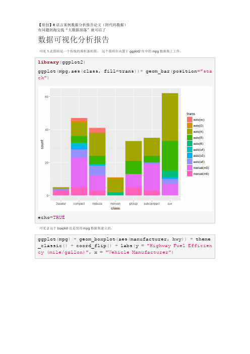
【原创】R语言数据可视化分析报告(附代码数据)
Vis 3这个图形是用另一个数据集菱形建立的,也是内置在ggplot2包中的数据集。
library(ggthemes)
ggplot(diamonds)+geom_density(aes(price,fill=cut,color=cut),alpha=0.4,size=0.5)+labs(title='Diamond Price Density',x='Diamond Price (USD)',y='Density')+theme_economist()
library(ggplot2)
ggplot(mpg,aes(class,fill=trans))+geom_bar(position="stack")
echo=TRUE
可见2这个boxplot也是使用mpg数据集建立的。
ggplot(mpg)+geom_boxplot(aes(manufacturer,hwy))+theme_classic()+coord_flip()+labs(y="Highway Fuel Efficiency (mile/gallon)",x="Vehicle Manufacturer")
echo=TRUE
另外,我正在使用ggplot2软件包来将线性模型拟合到框架内的所有数据上。
ggplot(iris,aes(Sepal.Length,Petal.Length))+geom_point()+geom_smooth(method=lm)+theme_minimal()+theme(panel.grid.major=element_line(size=1),panel.grid.minor=element_line(size=0.7))+labs(title='relationship between Petal and Sepal Length',x='Iris Sepal Length',y='Iris Petal Length')
【原创】r语言房价回归分析代码
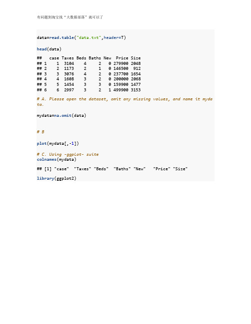
data=read.table("data.txt",header=T)head(data)## case Taxes Beds Baths New Price Size## 1 1 3104 4 2 0 279900 2048## 2 2 1173 2 1 0 146500 912## 3 3 3076 4 2 0 237700 1654## 4 4 1608 3 2 0 200000 2068## 5 5 1454 3 3 0 159900 1477## 6 6 2997 3 2 1 499900 3153# A. Please open the dataset, omit any missing values, and name it myda ta.mydata=na.omit(data)# Bplot(mydata[,-1])# C. Using -ggplot- suitecolnames(mydata)## [1] "case""Taxes""Beds""Baths""New""Price""Size"library(ggplot2)ggplot(mydata, aes(x = Size, y = Price)) + geom_point(aes( )) +geom_smooth()ggplot(mydata, aes(x = Taxes, y = Price)) +geom_point(aes( )) +geom_smooth()# D. Do your visualizations show a positive, negative,# or no relationship?# E. Is there evidence that you may need to transform any of your varia bles? Why? Motivate# your answer by showing any relevant statistics or graphsggplot(mydata, aes(x =(Size) , y =log(Price))) +geom_point(aes( )) +geom_smooth()ggplot(mydata, aes(x = (Taxes), y =log(Price))) + geom_point(aes( )) +geom_smooth()attach(mydata)cor(Taxes,Price)## [1] 0.8419802cor( (Taxes)^2 , (Price))## [1] 0.856277# F. Transform any variables as necessary. Explain your decisions. If y ou transformed any# of the variables, make additional visualizations of the relationship between the new# variable and the dependent variableggplot(mydata, aes(x = (Taxes^2), y =log(Price))) +geom_point(aes( )) +geom_smooth()# G. Estimate the correlation between any continuous independent variab les and the dependent variable.# What do they mean?cor(data[,-1])## Taxes Beds Baths New Price Size ## Taxes 1.0000000 0.47392873 0.5948543 0.38087410 0.8419802 0.8187958 ## Beds 0.4739287 1.00000000 0.4922224 0.04931556 0.3939570 0.5447831## Baths 0.5948543 0.49222235 1.0000000 0.25148095 0.5582533 0.6582247 ## New 0.3808741 0.04931556 0.2514810 1.00000000 0.4732608 0.3843277 ## Price 0.8419802 0.39395702 0.5582533 0.47326080 1.0000000 0.8337848 ## Size 0.8187958 0.54478311 0.6582247 0.38432773 0.8337848 1.0000000 # H. Fit a multiple regression to the data. Notice that your coefficien ts are really large, as# the dependent variable is measured in dollars. The norm is to rescale such dependent# variables (divide price by 1000), so that the coefficients are smalle r.summary(lm(Price~.,data=data[,-1]))#### Call:## lm(formula = Price ~ ., data = data[, -1])#### Residuals:## Min 1Q Median 3Q Max## -182112 -24377 -2046 21306 161870#### Coefficients:## Estimate Std. Error t value Pr(>|t|)## (Intercept) 4525.753 24474.054 0.185 0.8537## Taxes 38.135 6.815 5.596 2.16e-07 ***## Beds -11259.061 9115.003 -1.235 0.2198## Baths -2114.372 11465.113 -0.184 0.8541## New 41711.428 16887.196 2.470 0.0153 *## Size 68.350 13.936 4.904 3.92e-06 ***## ---## Signif. codes: 0 '***' 0.001 '**' 0.01 '*' 0.05 '.' 0.1 ' ' 1#### Residual standard error: 47240 on 94 degrees of freedom## Multiple R-squared: 0.7934, Adjusted R-squared: 0.7824## F-statistic: 72.19 on 5 and 94 DF, p-value: < 2.2e-16summary(lm(Price/1000~.,data=data[,-1]))#### Call:## lm(formula = Price/1000 ~ ., data = data[, -1])#### Residuals:## Min 1Q Median 3Q Max## -182.112 -24.377 -2.046 21.306 161.870#### Coefficients:## Estimate Std. Error t value Pr(>|t|)## (Intercept) 4.525753 24.474054 0.185 0.8537## Taxes 0.038135 0.006815 5.596 2.16e-07 ***## Beds -11.259061 9.115003 -1.235 0.2198## Baths -2.114372 11.465113 -0.184 0.8541## New 41.711428 16.887196 2.470 0.0153 *## Size 0.068350 0.013936 4.904 3.92e-06 ***## ---## Signif. codes: 0 '***' 0.001 '**' 0.01 '*' 0.05 '.' 0.1 ' ' 1#### Residual standard error: 47.24 on 94 degrees of freedom## Multiple R-squared: 0.7934, Adjusted R-squared: 0.7824## F-statistic: 72.19 on 5 and 94 DF, p-value: < 2.2e-16# I. Interpret the intercept and each of the coefficients.# J. Do the results make sense theoretically? Why or why not? If you fi nd that some of the# result do not make sense theoretically# K. Regress Price on Beds and Newsummary(mk<-lm(Price~Baths +New,data=data[,-1]))#### Call:## lm(formula = Price ~ Baths + New, data = data[, -1])#### Residuals:## Min 1Q Median 3Q Max## -154619 -52868 -9093 29513 287907#### Coefficients:## Estimate Std. Error t value Pr(>|t|)## (Intercept) -21355 28228 -0.757 0.451## Baths 83724 14143 5.920 4.87e-08 ***## New 114425 25506 4.486 1.99e-05 ***## ---## Signif. codes: 0 '***' 0.001 '**' 0.01 '*' 0.05 '.' 0.1 ' ' 1#### Residual standard error: 77240 on 97 degrees of freedom## Multiple R-squared: 0.4299, Adjusted R-squared: 0.4182## F-statistic: 36.58 on 2 and 97 DF, p-value: 1.454e-12predict(mk,data.frame(Baths=1:5,New=1),interval="confidence",level =0.9 )## fit lwr upr## 1 176794.4 126578.3 227010.5## 2 260518.5 220910.7 300126.4## 3 344242.6 302778.9 385706.3## 4 427966.7 373441.3 482492.2## 5 511690.8 438683.0 584698.6predict(mk,data.frame(Baths=1:5,New=0),interval="confidence",level =0.9 )## fit lwr upr## 1 62369.07 37034.79 87703.35## 2 146093.18 132333.24 159853.11## 3 229817.28 200831.47 258803.10## 4 313541.39 262606.62 364476.16## 5 397265.50 323428.81 471102.19# L. Repeat the steps in the previous answer to make a graph of predict ed values and the# 90% confidence interval around them for each number of bedrooms, assu ming that the# house is an old construction.# M. Put the two graphs side-by-side in your text document. What do the y tell you?preds=predict(mk,data.frame(Baths=1:5,New=1),interval="confidence", level =0.9 )plot( 1:5, preds[ ,1],xlab="Baths",type="l",main="Predicted Prices for New Consruction")# intervalslines(1:5, preds[ ,3], lty ='dashed', col ='red')lines(1:5, preds[ ,2], lty ='dashed', col ='red')preds=predict(mk,data.frame(Baths=1:5,New=0),interval="confidence", level =0.9 )# plotplot( 1:5, preds[ ,1],xlab="Baths",type="l",main="Predicted Prices for Old Consruction")# model# intervalslines(1:5, preds[ ,3], lty ='dashed', col ='red')lines(1:5, preds[ ,2], lty ='dashed', col ='red')# N. Make graphs that look exactly like the ones presented in Figure 1.。
- 1、下载文档前请自行甄别文档内容的完整性,平台不提供额外的编辑、内容补充、找答案等附加服务。
- 2、"仅部分预览"的文档,不可在线预览部分如存在完整性等问题,可反馈申请退款(可完整预览的文档不适用该条件!)。
- 3、如文档侵犯您的权益,请联系客服反馈,我们会尽快为您处理(人工客服工作时间:9:00-18:30)。
## BsmtFinType1 MasVnrType MasVnrArea MSZoning Utilities
## 79 24 23 4 2
## BsmtFullBath BsmtHalfBath Functional Exterior1st Exterior2nd
## Loaded glmnet 2.0-13
library(xgboost)
##
## Attaching package: 'xgboost'
## The following object is masked from 'package:dplyr':
##
## slice
Import the data and create a combined data set.
PoolQC
PoolQC中缺少2909个。 我们推断的原因是大多数家庭没有泳池。 所以我们将看到是否有任何PoolArea不是0与NA池QC。 然后我们根据PoolArea填充三个PoolQC,另一个填充没有。
poolna=which(is.na(full$PoolQC))
full[(full$PoolArea)>0&is.na(full$PoolQC),c("PoolArea","PoolQC")]
## # A tibble: 4 x 3
## PoolQC mean count
## <chr> <dbl> <int>
## 1 Ex 359.7500000 4
## 2 Fa 583.5000000 2
## 3 Gd 648.5000000 4
## 4 <NA> 0.4719835 2909
full$PoolQC[c(2421,2504)]="Ex";full$PoolQC[2600]="Fa"
## The following objects are masked from 'package:stats':
##
## filter, lag
## The following objects are masked from 'package:base':
##
## intersect, setdiff, setequal, union
## 2909 2814 2721 2348 1420
## LotFrontage GarageYrBlt GarageFinish GarageQual GarageCond
## 486 159 159 159 159
## GarageType BsmtCond BsmtExposure BsmtQual BsmtFinType2
misna=which(is.na(full$MiscFeature))
full[full$MiscVal>0&is.na(full$MiscFeature),c("MiscFeature","MiscVal")]
## MiscFeature MiscVal
## 2550 <NA> 17000
head(full[order(-full$MiscVal),c("MiscFeature","MiscVal")],10)
library(ggplot2)
library(mice)
library(e1071)
library(caret)
## Loading required package: lattice
library(glmnet)
## Loading required package: Matrix
## Loading required package: foreach
full$PoolQC[is.na(full$PoolQC)]="None"
MiscFeature
当我们谈论MiscFeature时,只有一个MiscVal> 0与NA MiscFeature。 通过MiscVal对数据进行排序,我们发现最广泛的MiscVal来自第二个车库。 所以我们用“Gar2”填写了丢失的MiscFeature。
## MiscFeature MiscVal
## 2550 <NA> 17000
## 347 Gar2 15500
## 1462 Gar2 12500
## 1231 Gar2 8300
## 2074 Othr 6500
## 2170 Shed 4500
## 2791 Gar2 4500
## 706 Othr 3500
## 2195 Gar2 3000
## 2698 Othr 3000
full$MiscFeature[2550]="Gar2"
## PoolArea PoolQC
## 2421 368 <NA>
## 2504 444 <NA>
## 2600 561 <NA>
full%>%select(PoolArea,PoolQC)%>%group_by(PoolQC)%>%summarise(mean=mean(PoolArea),count=n())
R语言House Price预测房价分析报告
在这个分析中,我们将尝试预测房子的交易价格。 因为有这么多变量,一些收缩回归可能是很好的选择。 以下是分析过程
数据概述
填补费用
虚拟变量
正规化和标准化
建模与预测模型
Datbrary(dplyr)
##
## Attaching package: 'dplyr'
Browse the data
sort(names(full))
str(full)
nacol=which(colSums(is.na(full))>0)
sort(colSums(sapply(full[nacol],is.na)),decreasing=T)
## PoolQC MiscFeature Alley Fence FireplaceQu
## 2 2 2 1 1
## BsmtFinSF1 BsmtFinSF2 BsmtUnfSF TotalBsmtSF Electrical
## 1 1 1 1 1
## KitchenQual GarageCars GarageArea SaleType
## 1 1 1 1
Missing Value缺失值