Eta invariants as sliceness obstructions and their relation to Casson-Gordon invariants
BrainVoyager 处理retinotopic mapping的过程

BrainVoyager 处理retinotopic mapping的过程
实验设计
ring 79个TR(前10后5个TR为灰屏,中间是八种大小的圆环依次出现)
流程(忘了删除掉前几个文件了)
1.生成实验设计
生成.prt文件
有八种大小的圆环,我就建了8个条件,加上灰屏的条件(感觉条件太多啦是不是只选择其中几个圆环就行)
2.建立功能像工程FMR
3.FMR预处理
预处理之后出现的参数图
4.建立结构像工程VMR
分辨率被转换为1mm×1mm×1mm,生成了*_ISO*文件,下面的分析都是用3D_struct_ISO.vmr文件
5.结构像与功能像匹配
6.结构像坐标转换到TAL空间
AC点(下面AC-PC这一步没有做好,AC和PC点都选的不准确)
AC-PC plane(这一步我不会做,我在下面绿色线的图上用鼠标点,XYZ的坐标没有任何变化,不知道怎么设置XYZ的值)
PC点
AP(指导手册上说,AP的线索是当COR图刚刚要出现时,这个刚刚出现的程度我不明白,下面这几个点找的感觉都不准确)
PP
SP
IP
RP
LP
Save.TAL
ACPC->TAL
7.分割
分割之后的图像好奇怪,上面这幅图中正确的应该是显示人脑的吧?感觉不应该是空的,导致下面出现的图中都是空的
8.将分割后的皮层进行展开。
Shift invariant wavelet packet bases
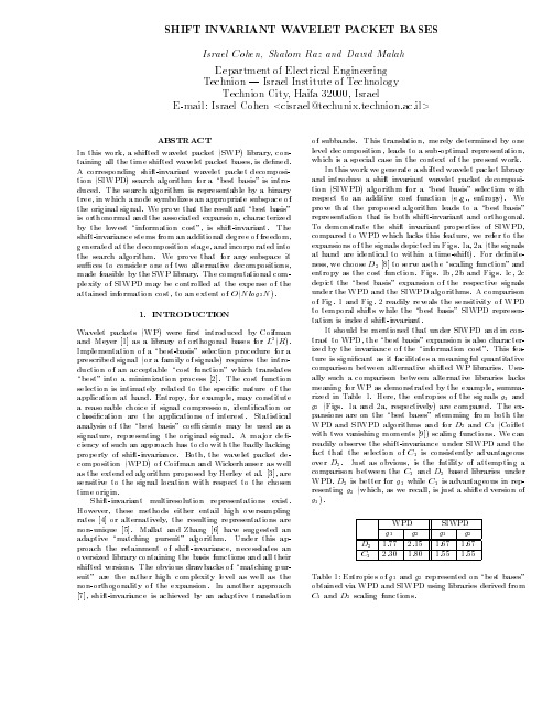
ABSTRACT
1. INTRODUCTION
Wavelet packets (WP) were rst introduced by Coifman and Meyer 1] as a library of orthogonal bases for L2 (R). Implementation of a \best-basis" selection procedure for a prescribed signal (or a family of signals) requires the introduction of an acceptable \cost function" which translates \best" into a minimization process 2]. The cost function selection is intimately related to the speci c nature of the application at hand. Entropy, for example, may constitute a reasonable choice if signal compression, identi cation or classi cation are the applications of interest. Statistical analysis of the \best basis" coe cients may be used as a signature, representing the original signal. A major de ciency of such an approach has to do with the badly lacking property of shift-invariance. Both, the wavelet packet decomposition (WPD) of Coifman and Wickerhauser as well as the extended algorithm proposed by Herley et al. 3], are sensitive to the signal location with respect to the chosen time origin. Shift-invariant multiresolution representations exist. However, these methods either entail high oversampling rates 4] or alternatively, the resulting representations are non-unique 5]. Mallat and Zhang 6] have suggested an adaptive \matching pursuit" algorithm. Under this approach the retainment of shift-invariance, necessitates an oversized library containing the basis functions and all their shifted versions. The obvious drawbacks of \matching pursuit" are the rather high complexity level as well as the non-orthogonality of the expansion. In another approach 7], shift-invariance is achieved by an adaptive translation
A New Approach of Image Denoising Based on Discrete Wavelet Transfer
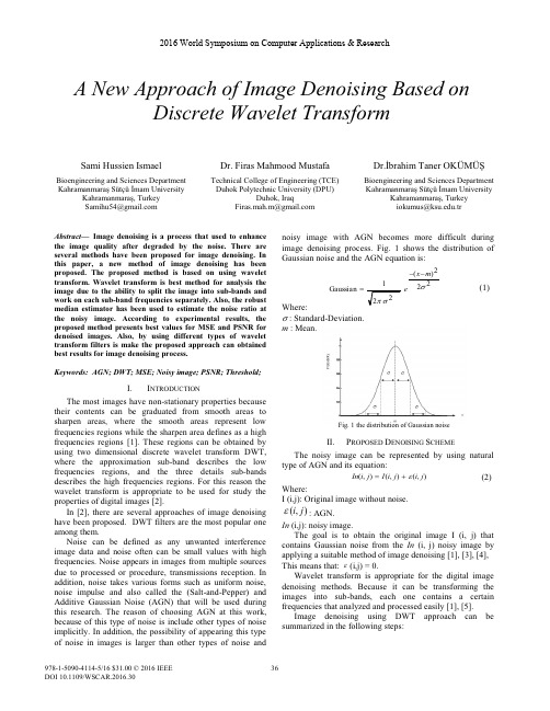
222)(2 21Gaussian V V S m x eA New Approach of Image Denoising Based onDiscrete Wavelet TransformSami Hussien IsmaelDr. Firas Mahmood MustafaDr.İbrahim Taner OKÜMÜŞBioengineering and Sciences Department Technical College of Engineering (TCE)Bioengineering and Sciences Department Kahramanmaraş Sütçü İmam UniversityDuhok Polytechnic University (DPU)Kahramanmaraş Sütçü İmam UniversityKahramanmaraş, Turkey Duhok, IraqKahramanmaraş, Turkey Samihu54@Firas.mah.m@iokumus@.trAbstract —Image denoising is a process that used to enhance the image quality after degraded by the noise. There are several methods have been proposed for image denoising. In this paper, a new method of image denoising has been proposed. The proposed method is based on using wavelet transform.W avelet transform is best method for analysis the image due to the ability to split the image into sub-bands and work on each sub-band frequencies separately. Also, the robust median estimator has been used to estimate the noise ratio at the noisy image. According to experimental results, the proposed method presents best values for MSE and PSNR for denoised images. Also, by using different types of wavelet transform filters is make the proposed approach can obtained best results for image denoising process.Keywords: AGN; DWT; MSE; Noisy image; PSNR; Threshold;I.I NTRODUCTIONThe most images have non-stationary properties because their contents can be graduated from smooth areas to sharpen areas, where the smooth areas represent low frequencies regions while the sharpen area defines as a high frequencies regions [1]. These regions can be obtained by using two dimensional discrete wavelet transform DWT,where the approximation sub-band describes the low frequencies regions, and the three details sub-bands describes the high frequencies regions. For this reason the wavelet transform is appropriate to be used for study the properties of digital images [2].In [2], there are several approaches of image denoising have been proposed. DWT filters are the most popular one among them.Noise can be defined as any unwanted interference image data and noise often can be small values with high frequencies. Noise appears in images from multiple sources due to processed or procedure, transmissions reception. In addition, noise takes various forms such as uniform noise, noise impulse and also called the (Salt-and-Pepper) and Additive Gaussian Noise (AGN) that will be used during this research. The reason of choosing AGN at this work, because of this type of noise is include other types of noise implicitly. In addition, the possibility of appearing this type of noise in images is larger than other types of noise andnoisy image with AGN becomes more difficult during image denoising process. Fig. 1 shows the distribution of Gaussian noise and the AGN equation is:(1) Where:V :Standard-Deviation. m :Mean.Fig. 1 the distribution of Gaussian noiseII.P ROPOSED D ENOISING S CHEMEThe noisy image can be represented by using natural type of AGN and its equation:),(),(),(j i j i I j i In H (2) Where:I (i,j): Original image without noise.),(j i H :AGN.In (i,j): noisy image.The goal is to obtain the original image I (i, j) that contains Gaussian noise from the In (i, j) noisy image by applying a suitable method of image denoising [1],[3],[4], This means that: H (i,j) = 0.Wavelet transform is appropriate for the digital image denoising methods. Because it can be transforming the images into sub-bands, each one contains a certain frequencies that analyzed and processed easily [1],[5].Image denoising using DWT approach can be summarized in the following steps:2016 World Symposium on Computer Applications & Research),(j i xc 1.Apply one level 2-dim DWT on noisy image (the noisy image divided into four sub-bands (Low-low LL, Low-high LH, High-low HL and High-high HH sub-bands). 2.Find the threshold value for each sub-band (LH, HL and HH).pare the threshold value of each sub-band with all pixel values of selected sub-band. If the pixel value less than threshold value, then set the pixel value to be zero. Otherwise, leave it and select the next pixel value. This step repeated until the last pixel value of selected sub-band.4.Apply one level inverse 2-dim DWT on the sub-bands to obtain a new image without noise.5.Find the values of mean square error (M SE) and peak signal-to-noise ratio (PSNR) for new image and original image to evaluate the proposed image denoising method. To compute the values of MSE and PSNR, the following equation is used:>@2101),(),(.1¦¦ M i N j j i I j i F N M MSE (3)MSEPSNR 2)255(log.10 (4)Where:I (i, j): Original image. F (i, j): New image M and N: size of image255: Max pixel value of grayscale image.The selection of the threshold value is important factor in decision making to delete or keep the pixel values of selected image sub-band [6]. Therefore, the threshold value must be high for denoising purpose and small value to maintain properties of the image. The threshold value can be found by applying the following equation [1].x Thx V V 2(5)Where:Thx : Threshold value.2V :Noise value of noisy image.x V :Standard deviation for one of these sub-bands (LH,HL and HH), and can be calculated by equation:NN i m i x ¦102)(V(6)The standard deviation value for each sub-band gives a uniform threshold value for its properties. TheVThthreshold value has an inverse relationship with thestandard deviation of the sub-band and it has positiverelationship with the standard deviation value of the noisyimage. In case (1 xV V) that means the pixel values of sub-band greater than the noise value. Therefore, the VThvalue must be select with minimum value to maintain the several properties of the pixel values of sub-band and denoise some pixel values of sub-band. While, in case (1!!xV V ) that means the pixel values of sub-band has a high value of noise. Therefore, the VTh must be select withmaximum value to denoise a several pixel values of sub-band and this can be lead to loss many properties of the pixel values of sub-band [1] .The noise power (2V ) can be computed by the estimation method that called (Robust Median Estimator) and applying the following formula [1].6745.0/),(j i x MedianV (7)Where x (i, j): represent analysis of diagonal sub-band for the first stage (HH or HL).In this paper, a new algorithm of image denoising has been proposed based on using DWT with two-stage of analysis. During the algorithm implementation, two grayscale images with sizes (256 × 256) that shown in Fig. 2 and noise type is additive Gaussian noise with zero rate (m = 0) and the standard deviation values (V =10, V =15, V =25). The four (LL, LH, HL and HH) sub-bands of the selected noisy image can be obtained by applying the 2-dim DWT.(a) Camera man (b) LenaFig. 2 the original imagesThe block diagram that shown in Fig. 3 is describe the image denoising process of the proposed method.The image denoising method not has any information about the amount of additive noise in contents of the noisy image. For this reason, the estimation method is used to estimate the amount of noise by using Robust M edian Estimator [1].After computing the noise value, 2-dim DWT with two stages is applied on the noisy image to obtain the (LH, HL, HH, LH1, HL1 and HH1) sub-bands. Then, the standard deviation for each sub-band is computed to use it in the equation (5) to calculate the threshold value for each sub-band and equation (8) is used for comparison process.°¿°¾½°¯°®t c otherwise Thx x j i x j i x ,0),,(),( (8)Where,),(j i x : The pixel values of noisy image sub-band. :The pixel value of denoised image.Finally, 2-dim inverse DWT with two stages is applied on these sub-bands to obtain denoised image.According to analysis of these sub-bands, the image denoising algorithm works on the following states:State 1: Apply one level 2-dim DWT on noisy image and compute Thx for these (LH, HL and HH) sub-bands. Then, the equation (8) is applied on all pixelvalues of these sub-bands. An inverse 2-dim DWTis applied on all sub-bands to construct a denoisedimage. Calculate M SE and PSNR between thedenoised image and original image.State 2: Obtain a (LL) sub-band by applying one level 2-dim DWT on the noisy image. And then apply 2-dim DWT on (LL) sub-band to obtain (LH1, HL1and HH1) sub-bands and calculate Thx for thesesub-bands. Then, equation (8) is applied on allpixel values of these sub-bands. To obtain thedenoised image an inverse 2-dim DWT is appliedon all pute M SE and PSNRbetween the denoised image and the original image. State 3: Apply one level 2-dim DWT on noisy image to obtain these (LH and HL) sub-bands, find their thxvalue by applying threshold method and set thepixel values of HH sub-band to be all zero values.Equation (8) is applied on (LH and HL) sub-bands.Then, apply an inverse 2-dim DWT for all sub-bands to construct a denoised image. CalculateM SE and PSNR between the denoised image andoriginal image.State 4: Obtain (LH)sub-band by applying one level 2-dim DWT on the noisy image, find its thx value byapplying threshold method and set the pixel valuesof (HL and HH) sub-bands to be all zero values.Equation (8) is applied on (LH) sub-band. Then, adenoised image can be obtained by applying aninverse 2-dim DWT on all sub-bands. Find M SEand PSNR values for the denoised image andoriginal image.State 5: Divide the noisy image into (LL, HL, LH and HH) sub-bands by applying one level 2-dim DWT.Then, compute thx value for (HL)sub-bands andset the pixel values of (LH and HH) sub-bands tobe all zero values. Equation (8) is applied on (HL)sub-band. Then, apply an inverse 2-dim DWT onall sub-bands to construct a denoised image.Compare between the denoised image and originalimage according to their MSE and PSNR values. State 6: One level 2-dim DWT is applied on noisy image to obtain (LL, HL, LH and HH) sub-bands. And then,set (HL, LH and HH) sub-bands to be all zerovalues.An inverse 2-dim DWT is applied on allsub-bands to construct a denoised image. CalculateM SE and PSNR between the denoised image andoriginal image.Fig. 3 the proposed method block diagramIII.E XPERIMENTAL R ESULTSM atlab technical programming language has been used to implement the proposed method. AGN is added to testoriginal image and the quantity of this noise must be notmore than a half amount of the standard deviation of theseoriginal images. Otherwise, if the noise amount is great thatmeans the denoising process will be remove more pixel values of the original image.The implementation results of proposed algorithm onCamera man image shows in Fig. 4 with the standard deviation is the (62.341). After AGN with values (V=10, V=15 and V=25) is added to it, the value of standard deviation has been became (62.928,63.459 and 65.211).Then, 2-dim DWT with one stage is applied on noisy imageto obtain high frequency sub-bands (HH, HL and LH). Toestimate the value of noise, equation (7) has been applied on (HH) sub-band and the estimation values of additive Gaussian noise for Camera man and Lena images tabulated in Table (1). By applying the equation (6) to obtain the threshold value Thx for each sub-band.Table 1: Standard deviation Std values for Camera man and Lenaimages using HH sub-bandImageStdoriginalimageStdNoise=10StdNoise=15StdNoise=25Stdestimation noise=10Stdestimation noise=15Stdestimation noise=25Cameraman62.34162.92863.45965.21111.02515.56624.723Lena52.29153.12454.19957.07010.71715.59024.416 According to experimental results for Camera man image that shown in Table (2), the proposed method at state (one sub-band deletion (HH) sub-band) has been achieved best results at noise ratio (V=10) and type of DWT filter is Rbior. While, in the state (all sub-band deletion), the proposed method has been achieved best results at the noise ratio (V=15 and V=25) and type of DWT filter is Sym.Fig. 4 Camera man image (a) Image with noise 10 (b)Denoised image without deleting level one (c)Denoised image without deleting level two (d)Denoised Image with HH sub-band deletion (e) Denoised image with HH and HL sub-bands deletion (f) Denoised image with HH, HL and LH sub-band deletion.Also, the proposed method is presented best values of PSNR for Camera man image with V =10 in state HH sub-band deletion among other states as shown in Fig. 5. While, in state all sub-bands deletion with V =15 and V =25, the proposed method presents best PSNR values for Camera man image as shown in Fig. 6 and Fig. 7.Fig .5 PSNR values for camera man image at V =10Table 3. shows the comparison of PSNR and M SEvalues for camera man image at two levels of DWT with V=10 between the proposed method and methods thatproposed in [7]. According to results, the proposed method is presented best PSNR and MSE values than methods thatproposed in [7].Table 2:MSE and PSNR values for Camera man image at different waveletfiltersImage Denoising MethodsOne analysis level Two analysis levelDelete HHDelete HH and HLDelete HH, HL and LH Filter NameMSE 88.24287.86281.71299.308104.782CoifPSNR 28.67428.69329.00828.16127.928MSE74.32374.32275.98594.347101.248BiorPSNR 29.42029.42029.32428.38428.077MSE 74.93174.76068.23294.37498.715RbioPSNR 29.38429.39429.79128.38228.187MSE 88.08287.88780.37389.94098.189dbPSNR 28.68228.69229.08028.59128.210MSE 87.49387.14480.42289.94096.324SymPSNR 28.71128.72829.07728.59128.293MSE 135.265140.929105.967118.99389.694HaarPSNR 26.81926.64127.87927.37628.603MSE167.161173.368104.085151.99788.546DmeyPSNR25.89925.74127.95726.31228.659Table 3. Comparison of PSNR and MSE values for Camera man image attwo levels of DWT with V =10.Also, Fig. 8 shows Lena image after the proposedmethod has been applied on it. Depending on the experimental results that shown in table 4,the proposed method at state (two sub-bands deletion (HH and LH) sub-bands has been achieved best results at noise ratio (V =10) and type of DWT filter is Bior 5.5 , While, in the state (all sub-band deletion), the proposed method has been achieved best results at the noise ratio (V =15) and type of DWT filter is Sym4, While, in the state (all sub-band deletion), the proposed method has been achieved best results at the noise ratio (V =25) and type of DWT filter is Sym5.Fig. 8 Lena image (a) Image with noise 10 (b) Denoised image without deleting level one (c) Denoised image without deleting level two (d)DWT LevelUniversal Threshold Visu Shrink Proposed Method MSEPSNRMSEPSNRMSEPSNR1st Level 564.92720.610548.29720.74074.32329.4202nd Level813.40319.027742.40319.42474.32229.420(a) (b) (c)(d) (e) (f)(a) (b) (c)(d) (e) (f)Denoised Image with HH sub-band deletion (e) Denoised image with HH and LH sub-bands deletion (f) Denoised image with HH, HL and LH sub-band deletion.In addition, the proposed algorithm is achieved best values of PSNR for Lena image with V =10 in state HH and LH sub-band deletion among other states as shown in Fig. 9. While, in state all sub-bands deletion with V =15 and V =25, the proposed method presents best PSNR values for Camera man image as shown in Fig. 10 and Fig. 11.Fig .9 PSNR values for Lena image at V =10Fig .10 PSNR values for Lena image at V =15Fig .11 PSNR values for Lena image at V =25IV.C ONCLUSIONIn this research, a new method of image denoising hasbeen proposed. The proposed method based on DWT that represents a best method for analysis the image due to the ability to split the image into sub-bands and work on each sub-band frequency separately. Also, the robust median estimator has been used to estimate the noise ratio in the noisy image. According to experimental results, the proposed method presents best values of MSE and PSNR for denoised images.Also, by using different types of wavelet transform filters is make the proposed approach can obtained best results for image denoising process.In future, the proposed method can be modified by more accurate estimation function to enhance its ability at image denoising process.Table 4: MSE and PSNR values for Lena image at different wavelet filtersImage Denoising MethodsOne analysis levelTwo analysis levelDelete HHDelete HH and LHDelete HH, HL and LHFilter NameMSE 94.26093.95482.27070.90971.284CoifPSNR 28.38828.40228.97829.62429.601MSE 82.60782.60472.92366.05069.927BiorPSNR 28.96128.96129.50229.93229.684MSE 82.09982.39767.25266.35571.962RbioPSNR28.98728.97229.85429.91229.560MSE 93.94693.77480.89468.56669.473dbPSNR 28.40228.41029.05229.77029.713MSE 93.89693.72280.89468.56669.712SymPSNR28.40428.41229.05229.77029.698MSE 94.450106.30977.64784.97096.829HaarPSNR28.37927.86529.23028.83828.271MSE 81.00692.72174.01582.61894.359DmeyPSNR29.04628.45929.43828.96028.383R EFERENCES[1]S. G. Chang, B. Yu, and M. Vetterli, “Adaptive Wavelet Thresholding for Image Denoising and Compression”, IEEE Transactions on Image Processing, vol. 9, no. 9, September 2000.[2]R. K. Rai, J. Asnani and T. R. Sontakke, “Review of Shrinkage Techniques for Image Denoising”, International Journal of Computer Applications (0975 – 8887), vol. 42, no.19, March 2012, pp. 13-16[3]P. Moulin, “Multiscale Image Decompositions and Wavelets”,Handbook of Image and Video Processing, 2nd edition, Academic Press, 2005[4] C.S. Burrus, R.A. Gopinath and H. GUO , “Introduction to Wavelets and Wavelet Transforms: A Primer ”. Prentice Hall, 1998.[5]A. Hamza and H. Krim, “Image Denoising: A Nonlinear Rob ust Statistical Approach”, IEEE Transactions on Signal Proce ssing, vol. 49, no. 12, pp. 3045-3054, December 2001.[6]A. Al Jumah, “Denoising of an Image Using Discrete Stationary Wavelet Transform and Various Thresholding Techniques”, Journal of Signal and Information Processing, vol. 4, pp.33-41, February 2013.[7]Anuta m and Rajni, “Performance Analysis of Image Denoising with Wavelet Thresholding M ethods For Different Levels of Decomposition”, The International Journal of Multimedia & Its Applications (IJMA) vol.6, no.3, pp.35-46, June 2014.P S NR。
a comparsion of affine region detectors

International Journal of Computer Vision 65(1/2), 43–72, 2005c 2005Springer Science +Business Media, Inc. Manufactured in The Netherlands.DOI:10.1007/s11263-005-3848-xA Comparison of Affine Region DetectorsK.MIKOLAJCZYKUniversity of Oxford,OX13PJ,Oxford,United Kingdomkm@T.TUYTELAARSUniversity of Leuven,Kasteelpark Arenberg10,3001Leuven,Belgiumtuytelaa@esat.kuleuven.beC.SCHMIDINRIA,GRAVIR-CNRS,655,av.de l’Europe,38330,Montbonnot,Franceschmid@inrialpes.frA.ZISSERMANUniversity of Oxford,OX13PJ,Oxford,United Kingdomaz@J.MATASCzech Technical University,Karlovo Namesti13,12135,Prague,Czech Republicmatas@cmp.felk.cvut.czF.SCHAFFALITZKY AND T.KADIRUniversity of Oxford,OX13PJ,Oxford,United Kingdomfsm@tk@L.V AN GOOLUniversity of Leuven,Kasteelpark Arenberg10,3001Leuven,Belgiumvangool@esat.kuleuven.beReceived August20,2004;Revised May3,2005;Accepted May11,2005First online version published in January,2006Abstract.The paper gives a snapshot of the state of the art in affine covariant region detectors,and compares their performance on a set of test images under varying imaging conditions.Six types of detectors are included: detectors based on affine normalization around Harris(Mikolajczyk and Schmid,2002;Schaffalitzky and Zisserman,2002)and Hessian points(Mikolajczyk and Schmid,2002),a detector of‘maximally stable extremal regions’,proposed by Matas et al.(2002);an edge-based region detector(Tuytelaars and Van Gool,1999) and a detector based on intensity extrema(Tuytelaars and Van Gool,2000),and a detector of‘salient regions’,44Mikolajczyk et al.proposed by Kadir,Zisserman and Brady(2004).The performance is measured against changes in viewpoint,scale, illumination,defocus and image compression.The objective of this paper is also to establish a reference test set of images and performance software,so that future detectors can be evaluated in the same framework.Keywords:affine region detectors,invariant image description,local features,performance evaluation1.IntroductionDetecting regions covariant with a class of transforma-tions has now reached some maturity in the computer vision literature.These regions have been used in quite varied applications including:wide baseline matching for stereo pairs(Baumberg,2000;Matas et al.,2002;Pritchett and Zisserman,1998;Tuytelaars and Van Gool,2000),reconstructing cameras for sets of disparate views(Schaffalitzky and Zisserman, 2002),image retrieval from large databases(Schmid and Mohr,1997;Tuytelaars and Van Gool,1999), model based recognition(Ferrari et al.,2004;Lowe, 1999;Obdrˇz´a lek and Matas,2002;Rothganger et al., 2003),object retrieval in video(Sivic and Zisserman, 2003;Sivic et al.,2004),visual data mining(Sivic and Zisserman,2004),texture recognition(Lazebnik et al.,2003a,b),shot location(Schaffalitzky and Zisserman,2003),robot localization(Se et al.,2002) and servoing(Tuytelaars et al.,1999),building panoramas(Brown and Lowe,2003),symmetry detection(Turina et al.,2001),and object categoriza-tion(Csurka et al.,2004;Dorko and Schmid,2003; Fergus et al.,2003;Opelt et al.,2004).The requirement for these regions is that they should correspond to the same pre-image for dif-ferent viewpoints,i.e.,their shape is notfixed but automatically adapts,based on the underlying image intensities,so that they are the projection of the same 3D surface patch.In particular,consider images from two viewpoints and the geometric transformation between the images induced by the viewpoint change. Regions detected after the viewpoint change should be the same,modulo noise,as the transformed versions of the regions detected in the original image–image transformation and region detection commute.As such,even though they have often been called invariant regions in the literature(e.g.,Dorko and Schmid,2003;Lazebnik et al.,2003a;Sivic and Zisserman,2004;Tuytelaars and Van Gool,1999),in principle they should be termed covariant regions since they change covariantly with the transformation. The confusion probably arises from the fact that,even though the regions themselves are covariant,the nor-malized image pattern they cover and the feature de-scriptors derived from them are typically invariant. Note,our use of the term‘region’simply refers to a set of pixels,i.e.any subset of the image.This differs from classical segmentation since the region bound-aries do not have to correspond to changes in image appearance such as colour or texture.All the detectors presented here produce simply connected regions,but in general this need not be the case.For viewpoint changes,the transformation of most interest is an affinity.This is illustrated in Fig.1. Clearly,a region withfixed shape(a circular exam-ple is shown in Fig.1(a)and(b))cannot cope with the geometric deformations caused by the change in view-point.We can observe that the circle does not cover the same image content,i.e.,the same physical surface. Instead,the shape of the region has to be adaptive,or covariant with respect to affinities(Fig.1(c)–close-ups shown in Fig.1(d)–(f)).Indeed,an affinity is suffi-cient to locally model image distortions arising from viewpoint changes,provided that(1)the scene sur-face can be locally approximated by a plane or in case of a rotating camera,and(2)perspective effects are ignored,which are typically small on a local scale any-way.Aside from the geometric deformations,also pho-tometric deformations need to be taken into account. These can be modeled by a linear transformation of the intensities.To further illustrate these issues,and how affine covariant regions can be exploited to cope with the geometric and photometric deformation between wide baseline images,consider the example shown in Fig.2.Unlike the example of Fig.1(where a circular region was chosen for one viewpoint)the elliptical image regions here are detected independently in each viewpoint.As is evident,the pre-images of these affineA Comparison of Affine Region Detectors45Figure 1.Class of transformations needed to cope with viewpoint changes.(a)First viewpoint;(b,c)second viewpoint.Fixed size circular patches (a,b)clearly do not suffice to deal with general viewpoint changes.What is needed is an anisotropic rescaling,i.e.,an affinity (c).Bottom row shows close-up of the images of the toprow.Figure 2.Affine covariant regions offer a solution to viewpoint and illumination changes.First row:one viewpoint;second row:other viewpoint.(a)Original images,(b)detected affine covariant regions,(c)close-up of the detected regions.(d)Geometric normalization to circles.The regions are the same up to rotation.(e)Photometric and geometric normalization.The slight residual difference in rotation is due to an estimation error.covariant regions correspond to the same surface region.Given such an affine covariant region,it is then possible to normalize against the geometric and photometric deformations (shown in Fig.2(d),(e))and to obtain a viewpoint and illumination invariant description of the intensity pattern within the region.In a typical matching application,the regions are used as follows.First,a set of covariant regions is46Mikolajczyk et al.detected in an image.Often a large number,perhaps hundreds or thousands,of possibly overlapping regions are obtained.A vector descriptor is then asso-ciated with each region,computed from the intensity pattern within the region.This descriptor is chosen to be invariant to viewpoint changes and,to some extent, illumination changes,and to discriminate between the regions.Correspondences may then be established with another image of the same scene,byfirst detect-ing and representing regions(independently)in the new image;and then matching the regions based on their descriptors.By design the regions commute with viewpoint change,so by design,corresponding regions in the two images will have similar(ideally identical) vector descriptors.The benefits are that correspon-dences can then be easily established and,since there are multiple regions,the method is robust to partial occlusions.This paper gives a snapshot of the state of the art in affine covariant region detection.We will describe and compare six methods of detecting these regions on images.These detectors have been designed and implemented by a number of researchers and the comparison is carried out using binaries supplied by the authors.The detectors are:(i)the ‘Harris-Affine’detector(Mikolajczyk and Schmid, 2002,2004;Schaffalitzky and Zisserman,2002); (ii)the‘Hessian-Affine’detector(Mikolajczyk and Schmid,2002,2004);(iii)the‘maximally stable extremal region’detector(or MSER,for short)(Matas et al.,2002,2004);(iv)an edge-based region detec-tor(Tuytelaars and Van Gool,1999,2004)(referred to as EBR);(v)an intensity extrema-based region detector(Tuytelaars and Van Gool,2000,2004) (referred to as IBR);and(vi)an entropy-based region detector(Kadir et al.,2004)(referred to as salient regions).To limit the scope of the paper we have not included methods for detecting regions which are covariant only to similarity transformations(i.e.,in particular scale), such as(Lowe,1999,2004;Mikolajczyk and Schmid, 2001;Mikolajczyk et al.,2003),or other methods of computing affine invariant descriptors,such as image lines connecting interest points(Matas et al.,2000; Tell and Carlson,2000,2002),or invariant vertical line segments(Goedeme et al.,2004).Also the detectors proposed by Lindeberg and G˚a rding(1997)and Baum-berg(2000)have not been included,as they come very close to the Harris-Affine and Hessian-Affine detectors.The six detectors are described in Section2.They are compared on the data set shown in Fig.9.This data set includes structured and textured scenes as well as different types of transformations:viewpoint changes,scale changes,illumination changes,blur and JPEG compression.It is described in more detail in Section3.Two types of comparisons are carried out. First,in Section10,the repeatability of the detector is measured:how well does the detector determine cor-responding scene regions?This is measured by com-paring the overlap between the ground truth and de-tected regions,in a manner similar to the evaluation test used in Mikolajczyk and Schmid(2002),but with special attention paid to the effect of the different scales (region sizes)of the various detectors’output.Here, we also measure the accuracy of the regions’shape, scale and localization.Second,the distinctiveness of the detected regions is assessed:how distinguishable are the regions detected?Following(Mikolajczyk and Schmid,2003,2005),we use the SIFT descriptor de-veloped by Lowe(1999),which is an128-dimensional vector,to describe the intensity pattern within the im-age regions.This descriptor has been demonstrated to be superior to others used in literature on a number of measures(Mikolajczyk and Schmid,2003).Our intention is that the images and tests de-scribed here will be a benchmark against which fu-ture affine covariant region detectors can be assessed. The images,Matlab code to carry out the performance tests,and binaries of the detectors are available from /∼vgg/research/affine. 2.Affine Covariant DetectorsIn this section we give a brief description of the six re-gion detectors used in the comparison.Section2.1de-scribes the related methods Harris-Affine and Hessian-Affine.Sections2.2and2.3describe methods for detecting edge-based regions and intensity extrema-based regions.Finally,Sections2.4and2.5describe MSER and salient regions.For the purpose of the comparisons the output re-gion of all detector types are represented by a common shape,which is an ellipse.Figures3and4show the el-lipses for all detectors on one pair of images.In order not to overload the images,only some of the corre-sponding regions that were actually detected in both images have been shown.This selection is obtained by increasing the threshold.A Comparison of Affine Region Detectors47Figure3.Regions generated by different detectors on corresponding sub-parts of thefirst and third graffiti images of Fig.9(a).The ellipses show the original detection size.In fact,for most of the detectors the output shape is an ellipse.However,for two of the de-tectors(edge-based regions and MSER)it is not, and information is lost by this representation,as ellipses can only be matched up to a rotational degree of freedom.Examples of the original re-gions detected by these two methods are given in Fig.5.These are parallelogram-shaped regions for the edge-based region detector,and arbitrarily shaped regions for the MSER detector.In the following the representing ellipse is chosen to have the same first and second moments as the originally detected region,which is an affine covariant construction method.48Mikolajczyk etal.Figure 4.Regions generated by different detectors continued.2.1.Detectors Based on Affine Normalization—Harris-Affine &Hessian-AffineWe describe here two related methods which detect interest points in scale-space,and then determine an elliptical region for each point.Interest points are either detected with the Harris detector or with a detector based on the Hessian matrix.In both casesscale-selection is based on the Laplacian,and the shape of the elliptical region is determined with the second moment matrix of the intensity gradient (Baumberg,2000;Lindeberg and G˚a rding,1997).The second moment matrix,also called the auto-correlation matrix,is often used for feature detection or for describing local image structures.Here it is used both in the Harris detector and the ellipticalA Comparison of Affine Region Detectors49Figure5.Originally detected region shapes for the regions shown in Figs.3(c)and4(b). shape estimation.This matrix describes the gradientdistribution in a local neighbourhood of a point:M=µ(x,σI,σD)= µ11µ12µ21µ22=σ2D g(σI)∗I2x(x,σD)I x I y(x,σD)I x I y(x,σD)I2y(x,σD)(1)The local image derivatives are computed with Gaussian kernels of scaleσD(differentiation scale). The derivatives are then averaged in the neighbourhood of the point by smoothing with a Gaussian window of scaleσI(integration scale).The eigenvalues of this matrix represent two principal signal changes in a neighbourhood of the point.This property enables the extraction of points,for which both curvatures are significant,that is the signal change is significant in orthogonal directions.Such points are stable in arbitrary lighting conditions and are representative of an image.One of the most reliable interest point detectors,the Harris detector(Harris and Stephens, 1988),is based on this principle.A similar idea is explored in the detector based on the Hessian matrix:H=H(x,σD)=h11h12h21h22=I xx(x,σD)I xy(x,σD)I xy(x,σD)I yy(x,σD)(2)The second derivatives,which are used in this matrix give strong responses on blobs and ridges.The regions are similar to those detected by a Laplacian operator (trace)(Lindeberg,1998;Lowe,1999)but a function based on the determinant of the Hessian matrix penal-izes very long structures for which the second deriva-tive in one particular orientation is very small.A local maximum of the determinant indicates the presence of a blob structure.To deal with scale changes a scale selection method(Lindeberg,1998)is applied.The idea is to select the characteristic scale of a local structure, for which a given function attains an extremum over scales(see Fig.6).The selected scale is characteristic in the quantitative sense,since it measures the scale50Mikolajczyk etal.Figure 6.Example of characteristic scales.Top row shows images taken with different zoom.Bottom row shows the responses of the Laplacian over scales.The characteristic scales are 10.1and 3.9for the left and right image,respectively.The ratio of scales corresponds to the scale factor (2.5)between the two images.The radius of displayed regions in the top row is equal to 3times the selected scales.at which there is maximum similarity between the feature detection operator and the local image struc-tures.The size of the region is therefore selected in-dependently of image resolution for each point.The Laplacian operator is used for scale selection in both detectors since it gave the best results in the ex-perimental comparison in Mikolajczyk and Schmid (2001).Given the set of initial points extracted at their char-acteristic scales we can apply the iterative estimation of elliptical affine region (Lindeberg and G˚a rding,1997).The eigenvalues of the second moment matrix are used to measure the affine shape of the point neighbourhood.To determine the affine shape,we find the transforma-tion that projects the affine pattern to the one with equal eigenvalues.This transformation is given by the square root of the second moment matrix M 1/2.If the neigh-bourhood of points x R and x L are normalized by trans-formations x R =M 1/2R x R and x L =M 1/2L x L ,respec-tively,the normalized regions are related by a simple rotation x L =R x R (Baumberg,2000;Lindeberg andG˚a rding,1997).The matrices M Land M R computed in the normalized frames are equal to a rotation matrix (see Fig.7).Note that rotation preserves the eigen-value ratio for an image patch,therefore,the affine deformation can be determined up to a rotation fac-tor.This factor can be recovered by other methods,for example normalization based on the dominant gradi-ent orientation (Lowe,1999;Mikolajczyk and Schmid,2002).The estimation of affine shape can be applied to any initial point given that the determinant of the second moment matrix is larger than zero and the signal to noise ratio is insignificant for this point.We can there-fore use this technique to estimate the shape of initial regions provided by the Harris and Hessian based de-tector.The outline of the iterative region estimation:1.Detect initial region with Harris or Hessian detector and select the scale.2.Estimate the shape with the second moment matrix3.Normalize the affine region to the circular one4.Go to step 2if the eigenvalues of the second moment matrix for new point are not equal.Examples of Harris-Affine and Hessian-Affine re-gions are displayed on Fig.3(a)and (b).2.2.An Edge-Based Region DetectorWe describe here a method to detect affine covariant regions in an image by exploiting the edges present in the image.The rationale behind this is that edges are typically rather stable features,that can be detected over a range of viewpoints,scales and/or illumination changes.Moreover,by exploiting the edge geometry,the dimensionality of the problem can be significantly reduced.Indeed,as will be shown next,the 6D search problem over all possible affinities (or 4D,once theA Comparison of Affine Region Detectors51Figure 7.Diagram illustrating the affine normalization using the second moment matrices.Image coordinates are transformed with matrices M −1/2L and M −1/2R .center point is fixed)can further be reduced to a one-dimensional problem by exploiting the nearby edges geometry.In practice,we start from a Harris corner point p (Harris and Stephens,1988)and a nearby edge,extracted with the Canny edge detector (Canny,1986).To increase the robustness to scale changes,these basic features are extracted at multiple scales.Two points p 1and p 2move away from the corner in both directions along the edge,as shown in Fig.8(a).Their relative speed is coupled through the equality of relative affine invariant parameters l 1and l 2:l i =absp i (1)(s i )p −p i (s i ) ds i (3)with s i an arbitrary curve parameter (in both direc-tions),p i (1)(s i )the first derivative of p i (s i )with respectto s i ,abs()the absolute value and |...|the determi-nant.This condition prescribes that the areas between the joint p ,p 1 and the edge and between the joint p ,p 2 and the edge remain identical.This is an affine invariant criterion indeed.From now on,we simply use l when referring to l 1=l 2.For each value l ,the two points p 1(1)and p 2(1)together with the corner p define a parallelogram (l ):the parallelogram spanned by the vectors p 1(l )−p and p 2(l )−p .This yields a one dimensional family of parallelogram-shaped regions as a function of l .From this 1D family we select one (or a few)parallelogram for which the following photometric quantities of the texture go through an extremum.Inv 1=abs|p 1−p g p 2−p g ||p −p 1p −p 2| M 100 M 200M 000−(M 100)2Inv 2=abs|p −p g q −p g |1p −p 2 M 100 M 200M 000−(M 100)2Figure 8.Construction methods for EBR and IBR.(a)The edge-based region detector starts from a corner point p and exploits nearby edgeinformation;(b)The intensity extrema-based region detector starts from an intensity extremum and studies the intensity pattern along rays emanating from this point.52Mikolajczyk et al.with M n pq =I n (x ,y )x p y q dxdy(4)p g = M 110M 100,M 101M 100with M n pq the n th order ,(p +q )th degree momentcomputed over the region (l ),p g the center of gravity of the region,weighted with intensity I (x ,y ),and q the corner of the parallelogram opposite to the corner point p (see Fig.8(a)).The second factor in these formula has been added to ensure invariance under an intensity offset.In the case of straight edges,the method described above cannot be applied,since l =0along the entire edge.Since intersections of two straight edges occur quite often,we cannot simply neglect this case.To cir-cumvent this problem,the two photometric quantities given in Eq.(4)are combined and locations where both functions reach a minimum value are taken to fix the parameters s 1and s 2along the straight edges.Moreover,instead of relying on the correct detection of the Harris corner point,we can simply use the straight lines intersection point instead.A more detailed expla-nation of this method can be found in Tuytelaars and Van Gool (1999,2004).Examples of detected regions are displayed in Fig.5(b).For easy comparison in the context of this paper,the parallelograms representing the invariant regions are replaced by the enclosed ellipses,as shown in Fig.4(b).However,in this way the orientation-information is lost,so it should be avoided in a practical application,as discussed in the beginning of Section 2.2.3.Intensity Extrema-Based Region DetectorHere we describe a method to detect affine covariant regions that starts from intensity extrema (detected at multiple scales),and explores the image around them in a radial way,delineating regions of arbitrary shape,which are then replaced by ellipses.More precisely,given a local extremum in inten-sity,the intensity function along rays emanating from the extremum is studied,as shown in Fig.8(b).The following function is evaluated along each ray:f I (t )=abs (I (t )−I 0)max t 0abs (I (t )−I 0)dt t,d with t an arbitrary parameter along the ray,I (t )the intensity at position t ,I 0the intensity value at the ex-tremum and d a small number which has been added to prevent a division by zero.The point for which this function reaches an extremum is invariant under affine geometric and linear photometric transforma-tions (given the ray).Typically,a maximum is reached at positions where the intensity suddenly increases or decreases.The function f I (t )is in itself already in-variant.Nevertheless,we select the points where this function reaches an extremum to make a robust selec-tion.Next,all points corresponding to maxima of f I (t )along rays originating from the same local extremum are linked to enclose an affine covariant region (see Fig.8(b)).This often irregularly-shaped region is re-placed by an ellipse having the same shape moments up to the second order.This ellipse-fitting is again an affine covariant construction.Examples of detected re-gions are displayed in Fig.4(a).More details about this method can be found in Tuytelaars and Van Gool (2000,2004).2.4.Maximally Stable Extremal Region DetectorA Maximally Stable Extremal Region (MSER)is aconnected component of an appropriately thresholded image.The word ‘extremal’refers to the property that all pixels inside the MSER have either higher (bright extremal regions)or lower (dark extremal regions)intensity than all the pixels on its outer boundary.The ‘maximally stable’in MSER describes the property optimized in the threshold selection process.The set of extremal regions E ,i.e.,the set of all connected components obtained by thresholding,has a number of desirable properties.Firstly,a mono-tonic change of image intensities leaves E unchanged,since it depends only on the ordering of pixel intensi-ties which is preserved under monotonic transforma-tion.This ensures that common photometric changes modelled locally as linear or affine leave E unaffected,even if the camera is non-linear (gamma-corrected).Secondly,continuous geometric transformations pre-serve topology–pixels from a single connected compo-nent are transformed to a single connected component.Thus after a geometric change locally approximated by an affine transform,homography or even continuous non-linear warping,a matching extremal region will be in the transformed set E .Finally,there are no more extremal regions than there are pixels in the image.SoA Comparison of Affine Region Detectors53a set of regions was defined that is preserved under a broad class of geometric and photometric changes and yet has the same cardinality as e.g.the set offixed-sized square windows commonly used in narrow-baseline matching.Implementation Details.The enumeration of the set of extremal regions E is very efficient,almost linear in the number of image pixels.The enumeration pro-ceeds as follows.First,pixels are sorted by intensity. After sorting,pixels are marked in the image(either in decreasing or increasing order)and the list of growing and merging connected components and their areas is maintained using the union-find algorithm(Sedgewick, 1988).During the enumeration process,the area of each connected component as a function of intensity is stored.Among the extremal regions,the‘maximally stable’ones are those corresponding to thresholds were the relative area change as a function of relative change of threshold is at a local minimum.In other words, the MSER are the parts of the image where local bi-narization is stable over a large range of thresholds. The definition of MSER stability based on relative area change is only affine invariant(both photomet-rically and geometrically).Consequently,the process of MSER detection is affine covariant.Detection of MSER is related to thresholding,since every extremal region is a connected component of a thresholded image.However,no global or‘optimal’threshold is sought,all thresholds are tested and the stability of the connected components evaluated.The output of the MSER detector is not a binarized image. For some parts of the image,multiple stable thresholds exist and a system of nested subsets is output in this case.Finally we remark that the different sets of extremal regions can be defined just by changing the ordering function.The MSER described in this section and used in the experiments should be more precisely called intensity induced MSERs.2.5.Salient Region DetectorThis detector is based on the pdf of intensity values computed over an elliptical region.Detection proceeds in two steps:first,at each pixel the entropy of the pdf is evaluated over the three parameter family of el-lipses centred on that pixel.The set of entropy extrema over scale and the corresponding ellipse parameters are recorded.These are candidate salient regions.Second,the candidate salient regions over the entire image are ranked using the magnitude of the derivative of the pdf with respect to scale.The top P ranked regions are retained.In more detail,the elliptical region E centred on a pixel x is parameterized by its scale s(which specifies the major axis),its orientationθ(of the major axis), and the ratio of major to minor axesλ.The pdf of intensities p(I)is computed over E.The entropy H is then given byH=−Ip(I)log p(I)The set of extrema over scale in H is computed for the parameters s,θ,λfor each pixel of the image.For each extrema the derivative of the pdf p(I;s,θ,λ)with s is computed asW=s22s−1I∂p(I;s,θ,λ)∂s,and the saliency Y of the elliptical region is com-puted as Y=HW.The regions are ranked by their saliency Y.Examples of detected regions are displayed in Fig.4(c).More details about this method can be found in Kadir et al.(2004).3.The Image Data SetFigure9shows examples from the image sets used to evaluate the detectors.Five different changes in imag-ing conditions are evaluated:viewpoint changes(a) &(b);scale changes(c)&(d);image blur(e)&(f); JPEG compression(g);and illumination(h).In the cases of viewpoint change,scale change and blur,the same change in imaging conditions is applied to two different scene types.This means that the effect of changing the image conditions can be separated from the effect of changing the scene type.One scene type contains homogeneous regions with distinctive edge boundaries(e.g.graffiti,buildings),and the other con-tains repeated textures of different forms.These will be referred to as structured versus textured scenes re-spectively.In the viewpoint change test the camera varies from a fronto-parallel view to one with significant fore-shortening at approximately60degrees to the camera. The scale change and blur sequences are acquired by varying the camera zoom and focus respectively.。
A Discriminatively Trained, Multiscale, Deformable Part Model
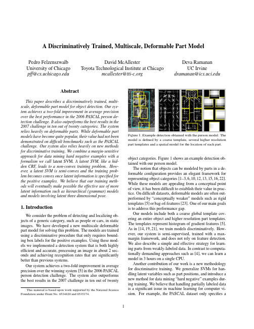
A Discriminatively Trained,Multiscale,Deformable Part ModelPedro Felzenszwalb University of Chicago pff@David McAllesterToyota Technological Institute at Chicagomcallester@Deva RamananUC Irvinedramanan@AbstractThis paper describes a discriminatively trained,multi-scale,deformable part model for object detection.Our sys-tem achieves a two-fold improvement in average precision over the best performance in the2006PASCAL person de-tection challenge.It also outperforms the best results in the 2007challenge in ten out of twenty categories.The system relies heavily on deformable parts.While deformable part models have become quite popular,their value had not been demonstrated on difficult benchmarks such as the PASCAL challenge.Our system also relies heavily on new methods for discriminative training.We combine a margin-sensitive approach for data mining hard negative examples with a formalism we call latent SVM.A latent SVM,like a hid-den CRF,leads to a non-convex training problem.How-ever,a latent SVM is semi-convex and the training prob-lem becomes convex once latent information is specified for the positive examples.We believe that our training meth-ods will eventually make possible the effective use of more latent information such as hierarchical(grammar)models and models involving latent three dimensional pose.1.IntroductionWe consider the problem of detecting and localizing ob-jects of a generic category,such as people or cars,in static images.We have developed a new multiscale deformable part model for solving this problem.The models are trained using a discriminative procedure that only requires bound-ing box labels for the positive ing these mod-els we implemented a detection system that is both highly efficient and accurate,processing an image in about2sec-onds and achieving recognition rates that are significantly better than previous systems.Our system achieves a two-fold improvement in average precision over the winning system[5]in the2006PASCAL person detection challenge.The system also outperforms the best results in the2007challenge in ten out of twenty This material is based upon work supported by the National Science Foundation under Grant No.0534820and0535174.Figure1.Example detection obtained with the person model.The model is defined by a coarse template,several higher resolution part templates and a spatial model for the location of each part. object categories.Figure1shows an example detection ob-tained with our person model.The notion that objects can be modeled by parts in a de-formable configuration provides an elegant framework for representing object categories[1–3,6,10,12,13,15,16,22]. While these models are appealing from a conceptual point of view,it has been difficult to establish their value in prac-tice.On difficult datasets,deformable models are often out-performed by“conceptually weaker”models such as rigid templates[5]or bag-of-features[23].One of our main goals is to address this performance gap.Our models include both a coarse global template cov-ering an entire object and higher resolution part templates. The templates represent histogram of gradient features[5]. As in[14,19,21],we train models discriminatively.How-ever,our system is semi-supervised,trained with a max-margin framework,and does not rely on feature detection. We also describe a simple and effective strategy for learn-ing parts from weakly-labeled data.In contrast to computa-tionally demanding approaches such as[4],we can learn a model in3hours on a single CPU.Another contribution of our work is a new methodology for discriminative training.We generalize SVMs for han-dling latent variables such as part positions,and introduce a new method for data mining“hard negative”examples dur-ing training.We believe that handling partially labeled data is a significant issue in machine learning for computer vi-sion.For example,the PASCAL dataset only specifies abounding box for each positive example of an object.We treat the position of each object part as a latent variable.We also treat the exact location of the object as a latent vari-able,requiring only that our classifier select a window that has large overlap with the labeled bounding box.A latent SVM,like a hidden CRF[19],leads to a non-convex training problem.However,unlike a hidden CRF, a latent SVM is semi-convex and the training problem be-comes convex once latent information is specified for thepositive training examples.This leads to a general coordi-nate descent algorithm for latent SVMs.System Overview Our system uses a scanning window approach.A model for an object consists of a global“root”filter and several part models.Each part model specifies a spatial model and a partfilter.The spatial model defines a set of allowed placements for a part relative to a detection window,and a deformation cost for each placement.The score of a detection window is the score of the root filter on the window plus the sum over parts,of the maxi-mum over placements of that part,of the partfilter score on the resulting subwindow minus the deformation cost.This is similar to classical part-based models[10,13].Both root and partfilters are scored by computing the dot product be-tween a set of weights and histogram of gradient(HOG) features within a window.The rootfilter is equivalent to a Dalal-Triggs model[5].The features for the partfilters are computed at twice the spatial resolution of the rootfilter. Our model is defined at afixed scale,and we detect objects by searching over an image pyramid.In training we are given a set of images annotated with bounding boxes around each instance of an object.We re-duce the detection problem to a binary classification prob-lem.Each example x is scored by a function of the form, fβ(x)=max zβ·Φ(x,z).Hereβis a vector of model pa-rameters and z are latent values(e.g.the part placements). To learn a model we define a generalization of SVMs that we call latent variable SVM(LSVM).An important prop-erty of LSVMs is that the training problem becomes convex if wefix the latent values for positive examples.This can be used in a coordinate descent algorithm.In practice we iteratively apply classical SVM training to triples( x1,z1,y1 ,..., x n,z n,y n )where z i is selected to be the best scoring latent label for x i under the model learned in the previous iteration.An initial rootfilter is generated from the bounding boxes in the PASCAL dataset. The parts are initialized from this rootfilter.2.ModelThe underlying building blocks for our models are the Histogram of Oriented Gradient(HOG)features from[5]. We represent HOG features at two different scales.Coarse features are captured by a rigid template covering anentireImage pyramidFigure2.The HOG feature pyramid and an object hypothesis de-fined in terms of a placement of the rootfilter(near the top of the pyramid)and the partfilters(near the bottom of the pyramid). detection window.Finer scale features are captured by part templates that can be moved with respect to the detection window.The spatial model for the part locations is equiv-alent to a star graph or1-fan[3]where the coarse template serves as a reference position.2.1.HOG RepresentationWe follow the construction in[5]to define a dense repre-sentation of an image at a particular resolution.The image isfirst divided into8x8non-overlapping pixel regions,or cells.For each cell we accumulate a1D histogram of gra-dient orientations over pixels in that cell.These histograms capture local shape properties but are also somewhat invari-ant to small deformations.The gradient at each pixel is discretized into one of nine orientation bins,and each pixel“votes”for the orientation of its gradient,with a strength that depends on the gradient magnitude.For color images,we compute the gradient of each color channel and pick the channel with highest gradi-ent magnitude at each pixel.Finally,the histogram of each cell is normalized with respect to the gradient energy in a neighborhood around it.We look at the four2×2blocks of cells that contain a particular cell and normalize the his-togram of the given cell with respect to the total energy in each of these blocks.This leads to a vector of length9×4 representing the local gradient information inside a cell.We define a HOG feature pyramid by computing HOG features of each level of a standard image pyramid(see Fig-ure2).Features at the top of this pyramid capture coarse gradients histogrammed over fairly large areas of the input image while features at the bottom of the pyramid capture finer gradients histogrammed over small areas.2.2.FiltersFilters are rectangular templates specifying weights for subwindows of a HOG pyramid.A w by hfilter F is a vector with w×h×9×4weights.The score of afilter is defined by taking the dot product of the weight vector and the features in a w×h subwindow of a HOG pyramid.The system in[5]uses a singlefilter to define an object model.That system detects objects from a particular class by scoring every w×h subwindow of a HOG pyramid and thresholding the scores.Let H be a HOG pyramid and p=(x,y,l)be a cell in the l-th level of the pyramid.Letφ(H,p,w,h)denote the vector obtained by concatenating the HOG features in the w×h subwindow of H with top-left corner at p.The score of F on this detection window is F·φ(H,p,w,h).Below we useφ(H,p)to denoteφ(H,p,w,h)when the dimensions are clear from context.2.3.Deformable PartsHere we consider models defined by a coarse rootfilter that covers the entire object and higher resolution partfilters covering smaller parts of the object.Figure2illustrates a placement of such a model in a HOG pyramid.The rootfil-ter location defines the detection window(the pixels inside the cells covered by thefilter).The partfilters are placed several levels down in the pyramid,so the HOG cells at that level have half the size of cells in the rootfilter level.We have found that using higher resolution features for defining partfilters is essential for obtaining high recogni-tion performance.With this approach the partfilters repre-sentfiner resolution edges that are localized to greater ac-curacy when compared to the edges represented in the root filter.For example,consider building a model for a face. The rootfilter could capture coarse resolution edges such as the face boundary while the partfilters could capture details such as eyes,nose and mouth.The model for an object with n parts is formally defined by a rootfilter F0and a set of part models(P1,...,P n) where P i=(F i,v i,s i,a i,b i).Here F i is afilter for the i-th part,v i is a two-dimensional vector specifying the center for a box of possible positions for part i relative to the root po-sition,s i gives the size of this box,while a i and b i are two-dimensional vectors specifying coefficients of a quadratic function measuring a score for each possible placement of the i-th part.Figure1illustrates a person model.A placement of a model in a HOG pyramid is given by z=(p0,...,p n),where p i=(x i,y i,l i)is the location of the rootfilter when i=0and the location of the i-th part when i>0.We assume the level of each part is such that a HOG cell at that level has half the size of a HOG cell at the root level.The score of a placement is given by the scores of eachfilter(the data term)plus a score of the placement of each part relative to the root(the spatial term), ni=0F i·φ(H,p i)+ni=1a i·(˜x i,˜y i)+b i·(˜x2i,˜y2i),(1)where(˜x i,˜y i)=((x i,y i)−2(x,y)+v i)/s i gives the lo-cation of the i-th part relative to the root location.Both˜x i and˜y i should be between−1and1.There is a large(exponential)number of placements for a model in a HOG pyramid.We use dynamic programming and distance transforms techniques[9,10]to compute the best location for the parts of a model as a function of the root location.This takes O(nk)time,where n is the number of parts in the model and k is the number of cells in the HOG pyramid.To detect objects in an image we score root locations according to the best possible placement of the parts and threshold this score.The score of a placement z can be expressed in terms of the dot product,β·ψ(H,z),between a vector of model parametersβand a vectorψ(H,z),β=(F0,...,F n,a1,b1...,a n,b n).ψ(H,z)=(φ(H,p0),φ(H,p1),...φ(H,p n),˜x1,˜y1,˜x21,˜y21,...,˜x n,˜y n,˜x2n,˜y2n,). We use this representation for learning the model parame-ters as it makes a connection between our deformable mod-els and linear classifiers.On interesting aspect of the spatial models defined here is that we allow for the coefficients(a i,b i)to be negative. This is more general than the quadratic“spring”cost that has been used in previous work.3.LearningThe PASCAL training data consists of a large set of im-ages with bounding boxes around each instance of an ob-ject.We reduce the problem of learning a deformable part model with this data to a binary classification problem.Let D=( x1,y1 ,..., x n,y n )be a set of labeled exam-ples where y i∈{−1,1}and x i specifies a HOG pyramid, H(x i),together with a range,Z(x i),of valid placements for the root and partfilters.We construct a positive exam-ple from each bounding box in the training set.For these ex-amples we define Z(x i)so the rootfilter must be placed to overlap the bounding box by at least50%.Negative exam-ples come from images that do not contain the target object. Each placement of the rootfilter in such an image yields a negative training example.Note that for the positive examples we treat both the part locations and the exact location of the rootfilter as latent variables.We have found that allowing uncertainty in the root location during training significantly improves the per-formance of the system(see Section4).tent SVMsA latent SVM is defined as follows.We assume that each example x is scored by a function of the form,fβ(x)=maxz∈Z(x)β·Φ(x,z),(2)whereβis a vector of model parameters and z is a set of latent values.For our deformable models we define Φ(x,z)=ψ(H(x),z)so thatβ·Φ(x,z)is the score of placing the model according to z.In analogy to classical SVMs we would like to trainβfrom labeled examples D=( x1,y1 ,..., x n,y n )by optimizing the following objective function,β∗(D)=argminβλ||β||2+ni=1max(0,1−y i fβ(x i)).(3)By restricting the latent domains Z(x i)to a single choice, fβbecomes linear inβ,and we obtain linear SVMs as a special case of latent tent SVMs are instances of the general class of energy-based models[18].3.2.Semi-ConvexityNote that fβ(x)as defined in(2)is a maximum of func-tions each of which is linear inβ.Hence fβ(x)is convex inβ.This implies that the hinge loss max(0,1−y i fβ(x i)) is convex inβwhen y i=−1.That is,the loss function is convex inβfor negative examples.We call this property of the loss function semi-convexity.Consider an LSVM where the latent domains Z(x i)for the positive examples are restricted to a single choice.The loss due to each positive example is now bined with the semi-convexity property,(3)becomes convex inβ.If the labels for the positive examples are notfixed we can compute a local optimum of(3)using a coordinate de-scent algorithm:1.Holdingβfixed,optimize the latent values for the pos-itive examples z i=argmax z∈Z(xi )β·Φ(x,z).2.Holding{z i}fixed for positive examples,optimizeβby solving the convex problem defined above.It can be shown that both steps always improve or maintain the value of the objective function in(3).If both steps main-tain the value we have a strong local optimum of(3),in the sense that Step1searches over an exponentially large space of latent labels for positive examples while Step2simulta-neously searches over weight vectors and an exponentially large space of latent labels for negative examples.3.3.Data Mining Hard NegativesIn object detection the vast majority of training exam-ples are negative.This makes it infeasible to consider all negative examples at a time.Instead,it is common to con-struct training data consisting of the positive instances and “hard negative”instances,where the hard negatives are data mined from the very large set of possible negative examples.Here we describe a general method for data mining ex-amples for SVMs and latent SVMs.The method iteratively solves subproblems using only hard instances.The innova-tion of our approach is a theoretical guarantee that it leads to the exact solution of the training problem defined using the complete training set.Our results require the use of a margin-sensitive definition of hard examples.The results described here apply both to classical SVMs and to the problem defined by Step2of the coordinate de-scent algorithm for latent SVMs.We omit the proofs of the theorems due to lack of space.These results are related to working set methods[17].We define the hard instances of D relative toβas,M(β,D)={ x,y ∈D|yfβ(x)≤1}.(4)That is,M(β,D)are training examples that are incorrectly classified or near the margin of the classifier defined byβ. We can show thatβ∗(D)only depends on hard instances. Theorem1.Let C be a subset of the examples in D.If M(β∗(D),D)⊆C thenβ∗(C)=β∗(D).This implies that in principle we could train a model us-ing a small set of examples.However,this set is defined in terms of the optimal modelβ∗(D).Given afixedβwe can use M(β,D)to approximate M(β∗(D),D).This suggests an iterative algorithm where we repeatedly compute a model from the hard instances de-fined by the model from the last iteration.This is further justified by the followingfixed-point theorem.Theorem2.Ifβ∗(M(β,D))=βthenβ=β∗(D).Let C be an initial“cache”of examples.In practice we can take the positive examples together with random nega-tive examples.Consider the following iterative algorithm: 1.Letβ:=β∗(C).2.Shrink C by letting C:=M(β,C).3.Grow C by adding examples from M(β,D)up to amemory limit L.Theorem3.If|C|<L after each iteration of Step2,the algorithm will converge toβ=β∗(D)infinite time.3.4.Implementation detailsMany of the ideas discussed here are only approximately implemented in our current system.In practice,when train-ing a latent SVM we iteratively apply classical SVM train-ing to triples x1,z1,y1 ,..., x n,z n,y n where z i is se-lected to be the best scoring latent label for x i under themodel trained in the previous iteration.Each of these triples leads to an example Φ(x i,z i),y i for training a linear clas-sifier.This allows us to use a highly optimized SVM pack-age(SVMLight[17]).On a single CPU,the entire training process takes3to4hours per object class in the PASCAL datasets,including initialization of the parts.Root Filter Initialization:For each category,we auto-matically select the dimensions of the rootfilter by looking at statistics of the bounding boxes in the training data.1We train an initial rootfilter F0using an SVM with no latent variables.The positive examples are constructed from the unoccluded training examples(as labeled in the PASCAL data).These examples are anisotropically scaled to the size and aspect ratio of thefilter.We use random subwindows from negative images to generate negative examples.Root Filter Update:Given the initial rootfilter trained as above,for each bounding box in the training set wefind the best-scoring placement for thefilter that significantly overlaps with the bounding box.We do this using the orig-inal,un-scaled images.We retrain F0with the new positive set and the original random negative set,iterating twice.Part Initialization:We employ a simple heuristic to ini-tialize six parts from the rootfilter trained above.First,we select an area a such that6a equals80%of the area of the rootfilter.We greedily select the rectangular region of area a from the rootfilter that has the most positive energy.We zero out the weights in this region and repeat until six parts are selected.The partfilters are initialized from the rootfil-ter values in the subwindow selected for the part,butfilled in to handle the higher spatial resolution of the part.The initial deformation costs measure the squared norm of a dis-placement with a i=(0,0)and b i=−(1,1).Model Update:To update a model we construct new training data triples.For each positive bounding box in the training data,we apply the existing detector at all positions and scales with at least a50%overlap with the given bound-ing box.Among these we select the highest scoring place-ment as the positive example corresponding to this training bounding box(Figure3).Negative examples are selected byfinding high scoring detections in images not containing the target object.We add negative examples to a cache un-til we encounterfile size limits.A new model is trained by running SVMLight on the positive and negative examples, each labeled with part placements.We update the model10 times using the cache scheme described above.In each it-eration we keep the hard instances from the previous cache and add as many new hard instances as possible within the memory limit.Toward thefinal iterations,we are able to include all hard instances,M(β,D),in the cache.1We picked a simple heuristic by cross-validating over5object classes. We set the model aspect to be the most common(mode)aspect in the data. We set the model size to be the largest size not larger than80%of thedata.Figure3.The image on the left shows the optimization of the la-tent variables for a positive example.The dotted box is the bound-ing box label provided in the PASCAL training set.The large solid box shows the placement of the detection window while the smaller solid boxes show the placements of the parts.The image on the right shows a hard-negative example.4.ResultsWe evaluated our system using the PASCAL VOC2006 and2007comp3challenge datasets and protocol.We refer to[7,8]for details,but emphasize that both challenges are widely acknowledged as difficult testbeds for object detec-tion.Each dataset contains several thousand images of real-world scenes.The datasets specify ground-truth bounding boxes for several object classes,and a detection is consid-ered correct when it overlaps more than50%with a ground-truth bounding box.One scores a system by the average precision(AP)of its precision-recall curve across a testset.Recent work in pedestrian detection has tended to report detection rates versus false positives per window,measured with cropped positive examples and negative images with-out objects of interest.These scores are tied to the reso-lution of the scanning window search and ignore effects of non-maximum suppression,making it difficult to compare different systems.We believe the PASCAL scoring method gives a more reliable measure of performance.The2007challenge has20object categories.We entered a preliminary version of our system in the official competi-tion,and obtained the best score in6categories.Our current system obtains the highest score in10categories,and the second highest score in6categories.Table1summarizes the results.Our system performs well on rigid objects such as cars and sofas as well as highly deformable objects such as per-sons and horses.We also note that our system is successful when given a large or small amount of training data.There are roughly4700positive training examples in the person category but only250in the sofa category.Figure4shows some of the models we learned.Figure5shows some ex-ample detections.We evaluated different components of our system on the longer-established2006person dataset.The top AP scoreaero bike bird boat bottle bus car cat chair cow table dog horse mbike person plant sheep sofa train tvOur rank 31211224111422112141Our score .180.411.092.098.249.349.396.110.155.165.110.062.301.337.267.140.141.156.206.336Darmstadt .301INRIA Normal .092.246.012.002.068.197.265.018.097.039.017.016.225.153.121.093.002.102.157.242INRIA Plus.136.287.041.025.077.279.294.132.106.127.067.071.335.249.092.072.011.092.242.275IRISA .281.318.026.097.119.289.227.221.175.253MPI Center .060.110.028.031.000.164.172.208.002.044.049.141.198.170.091.004.091.034.237.051MPI ESSOL.152.157.098.016.001.186.120.240.007.061.098.162.034.208.117.002.046.147.110.054Oxford .262.409.393.432.375.334TKK .186.078.043.072.002.116.184.050.028.100.086.126.186.135.061.019.036.058.067.090Table 1.PASCAL VOC 2007results.Average precision scores of our system and other systems that entered the competition [7].Empty boxes indicate that a method was not tested in the corresponding class.The best score in each class is shown in bold.Our current system ranks first in 10out of 20classes.A preliminary version of our system ranked first in 6classes in the official competition.BottleCarBicycleSofaFigure 4.Some models learned from the PASCAL VOC 2007dataset.We show the total energy in each orientation of the HOG cells in the root and part filters,with the part filters placed at the center of the allowable displacements.We also show the spatial model for each part,where bright values represent “cheap”placements,and dark values represent “expensive”placements.in the PASCAL competition was .16,obtained using a rigid template model of HOG features [5].The best previous re-sult of.19adds a segmentation-based verification step [20].Figure 6summarizes the performance of several models we trained.Our root-only model is equivalent to the model from [5]and it scores slightly higher at .18.Performance jumps to .24when the model is trained with a LSVM that selects a latent position and scale for each positive example.This suggests LSVMs are useful even for rigid templates because they allow for self-adjustment of the detection win-dow in the training examples.Adding deformable parts in-creases performance to .34AP —a factor of two above the best previous score.Finally,we trained a model with partsbut no root filter and obtained .29AP.This illustrates the advantage of using a multiscale representation.We also investigated the effect of the spatial model and allowable deformations on the 2006person dataset.Recall that s i is the allowable displacement of a part,measured in HOG cells.We trained a rigid model with high-resolution parts by setting s i to 0.This model outperforms the root-only system by .27to .24.If we increase the amount of allowable displacements without using a deformation cost,we start to approach a bag-of-features.Performance peaks at s i =1,suggesting it is useful to constrain the part dis-placements.The optimal strategy allows for larger displace-ments while using an explicit deformation cost.The follow-Figure 5.Some results from the PASCAL 2007dataset.Each row shows detections using a model for a specific class (Person,Bottle,Car,Sofa,Bicycle,Horse).The first three columns show correct detections while the last column shows false positives.Our system is able to detect objects over a wide range of scales (such as the cars)and poses (such as the horses).The system can also detect partially occluded objects such as a person behind a bush.Note how the false detections are often quite reasonable,for example detecting a bus with the car model,a bicycle sign with the bicycle model,or a dog with the horse model.In general the part filters represent meaningful object parts that are well localized in each detection such as the head in the person model.Figure6.Evaluation of our system on the PASCAL VOC2006 person dataset.Root uses only a rootfilter and no latent place-ment of the detection windows on positive examples.Root+Latent uses a rootfilter with latent placement of the detection windows. Parts+Latent is a part-based system with latent detection windows but no rootfilter.Root+Parts+Latent includes both root and part filters,and latent placement of the detection windows.ing table shows AP as a function of freely allowable defor-mation in thefirst three columns.The last column gives the performance when using a quadratic deformation cost and an allowable displacement of2HOG cells.s i01232+quadratic costAP.27.33.31.31.345.DiscussionWe introduced a general framework for training SVMs with latent structure.We used it to build a recognition sys-tem based on multiscale,deformable models.Experimental results on difficult benchmark data suggests our system is the current state-of-the-art in object detection.LSVMs allow for exploration of additional latent struc-ture for recognition.One can consider deeper part hierar-chies(parts with parts),mixture models(frontal vs.side cars),and three-dimensional pose.We would like to train and detect multiple classes together using a shared vocab-ulary of parts(perhaps visual words).We also plan to use A*search[11]to efficiently search over latent parameters during detection.References[1]Y.Amit and A.Trouve.POP:Patchwork of parts models forobject recognition.IJCV,75(2):267–282,November2007.[2]M.Burl,M.Weber,and P.Perona.A probabilistic approachto object recognition using local photometry and global ge-ometry.In ECCV,pages II:628–641,1998.[3] D.Crandall,P.Felzenszwalb,and D.Huttenlocher.Spatialpriors for part-based recognition using statistical models.In CVPR,pages10–17,2005.[4] D.Crandall and D.Huttenlocher.Weakly supervised learn-ing of part-based spatial models for visual object recognition.In ECCV,pages I:16–29,2006.[5]N.Dalal and B.Triggs.Histograms of oriented gradients forhuman detection.In CVPR,pages I:886–893,2005.[6] B.Epshtein and S.Ullman.Semantic hierarchies for recog-nizing objects and parts.In CVPR,2007.[7]M.Everingham,L.Van Gool,C.K.I.Williams,J.Winn,and A.Zisserman.The PASCAL Visual Object Classes Challenge2007(VOC2007)Results./challenges/VOC/voc2007/workshop.[8]M.Everingham, A.Zisserman, C.K.I.Williams,andL.Van Gool.The PASCAL Visual Object Classes Challenge2006(VOC2006)Results./challenges/VOC/voc2006/results.pdf.[9]P.Felzenszwalb and D.Huttenlocher.Distance transformsof sampled functions.Cornell Computing and Information Science Technical Report TR2004-1963,September2004.[10]P.Felzenszwalb and D.Huttenlocher.Pictorial structures forobject recognition.IJCV,61(1),2005.[11]P.Felzenszwalb and D.McAllester.The generalized A*ar-chitecture.JAIR,29:153–190,2007.[12]R.Fergus,P.Perona,and A.Zisserman.Object class recog-nition by unsupervised scale-invariant learning.In CVPR, 2003.[13]M.Fischler and R.Elschlager.The representation andmatching of pictorial structures.IEEE Transactions on Com-puter,22(1):67–92,January1973.[14] A.Holub and P.Perona.A discriminative framework formodelling object classes.In CVPR,pages I:664–671,2005.[15]S.Ioffe and D.Forsyth.Probabilistic methods forfindingpeople.IJCV,43(1):45–68,June2001.[16]Y.Jin and S.Geman.Context and hierarchy in a probabilisticimage model.In CVPR,pages II:2145–2152,2006.[17]T.Joachims.Making large-scale svm learning practical.InB.Sch¨o lkopf,C.Burges,and A.Smola,editors,Advances inKernel Methods-Support Vector Learning.MIT Press,1999.[18]Y.LeCun,S.Chopra,R.Hadsell,R.Marc’Aurelio,andF.Huang.A tutorial on energy-based learning.InG.Bakir,T.Hofman,B.Sch¨o lkopf,A.Smola,and B.Taskar,editors, Predicting Structured Data.MIT Press,2006.[19] A.Quattoni,S.Wang,L.Morency,M.Collins,and T.Dar-rell.Hidden conditional randomfields.PAMI,29(10):1848–1852,October2007.[20] ing segmentation to verify object hypothe-ses.In CVPR,pages1–8,2007.[21] D.Ramanan and C.Sminchisescu.Training deformablemodels for localization.In CVPR,pages I:206–213,2006.[22]H.Schneiderman and T.Kanade.Object detection using thestatistics of parts.IJCV,56(3):151–177,February2004. [23]J.Zhang,M.Marszalek,zebnik,and C.Schmid.Localfeatures and kernels for classification of texture and object categories:A comprehensive study.IJCV,73(2):213–238, June2007.。
二维巴特沃斯滤波器c语言

二维巴特沃斯滤波器1. 简介二维巴特沃斯滤波器是一种常用的图像处理方法,用于对图像进行频域滤波。
它基于巴特沃斯滤波器的原理,在频域中对图像进行平滑或增强。
本文将详细介绍二维巴特沃斯滤波器的原理、实现步骤以及应用案例。
2. 巴特沃斯滤波器原理巴特沃斯滤波器是一种频率域滤波器,通过调整截止频率和阶数来控制信号的频率响应。
其传输函数可以表示为:H (u,v )=11+(D (u,v )D 0)2n其中,D (u,v ) 是图像中每个点到中心点的距离,D 0 是截止频率,n 是阶数。
当 n 取不同值时,巴特沃斯滤波器可以实现不同程度的平滑或增强效果。
当 n >1 时,增加了阶数可以使得低频信号更加平坦;当 n <1 时,减小了阶数可以使得低频信号更加突出。
3. 实现步骤二维巴特沃斯滤波器的实现步骤如下:步骤 1:读取图像首先,需要从文件中读取待处理的图像。
可以使用 C 语言中的图像处理库,如 OpenCV ,来实现图像读取功能。
#include <opencv2/opencv.hpp>int main() {// 读取图像cv::Mat image = cv::imread("input.jpg", cv::IMREAD_GRAYSCALE);// 其他处理步骤...return 0;}步骤 2:进行傅里叶变换将读取的图像进行傅里叶变换,得到频域表示。
可以使用 OpenCV 提供的函数dft 来实现傅里叶变换。
#include <opencv2/opencv.hpp>int main() {// 读取图像cv::Mat image = cv::imread("input.jpg", cv::IMREAD_GRAYSCALE);// 进行傅里叶变换cv::Mat frequencyDomain;cv::dft(image, frequencyDomain, cv::DFT_COMPLEX_OUTPUT);// 其他处理步骤...return 0;}步骤 3:生成巴特沃斯滤波器根据巴特沃斯滤波器的传输函数公式,可以生成巴特沃斯滤波器的频域表示。
中心切片定理证明
中心切片定理证明中心切片定理(Central Slice Theorem)是计算机断层扫描图像重建(CT重建)的基础理论之一。
它是由托马斯·费博迪(Thomas S. Furry)于1948年首次提出的,也被称为费氏切片定理(Fubini's Slice Theorem)或费博迪切片定理(Fubini's Slice Theorem)。
中心切片定理是计算机断层扫描技术成像的核心原理之一,对于医学影像学、计算机辅助设计与制造等领域具有重要应用价值。
中心切片定理的基本思想是:在二维平面上对一个物体进行扫描,可以得到一组平行于扫描平面的切片图像。
这些切片图像包含了物体在不同位置上的信息,但由于切片之间的间隔较大,无法获得物体某些区域的细节信息。
而中心切片定理则提供了一种通过限制扫描角度范围来增加切片图像数量和密度的方法,从而实现对物体的更准确重建。
为了简化问题,我们首先讨论在二维平面上的情况。
假设有一个二维物体位于平面上,我们可以通过不同的角度进行扫描,得到一系列投影数据。
为了方便起见,我们假设物体在平面上是完全透明的,即完全没有吸收或衰减。
根据光学的等效原理,如果我们将透明平板放在投影数据中,它将产生与原始物体相同的投影数据。
现在,我们将考虑在一个固定角度上进行的扫描,并使用一个探测器来测量通过物体的平行光束的强度。
我们假设我们进行的扫描是从正上方进行的,即探测器位于物体的上方,光源位于物体的下方。
我们可以将探测器上各个点的强度测量数据连接起来,得到一个探测器的强度图。
现在,我们将探测器的位置旋转一定角度,并记录相应的探测器强度图。
通过不同角度的扫描,我们可以得到一系列探测器强度图,这些图像对应于不同的切片位置。
根据中心切片定理,我们可以通过这些探测器强度图来重建物体的密度分布。
中心切片定理的数学推导需要引入一些复杂的数学工具和方法,例如傅里叶变换和Radon变换等。
这超出了本文的讨论范围,我们只简单介绍一下中心切片定理的基本原理。
T.W. ANDERSON (1971). The Statistical Analysis of Time Series. Series in Probability and Ma
425 BibliographyH.A KAIKE(1974).Markovian representation of stochastic processes and its application to the analysis of autoregressive moving average processes.Annals Institute Statistical Mathematics,vol.26,pp.363-387. B.D.O.A NDERSON and J.B.M OORE(1979).Optimal rmation and System Sciences Series, Prentice Hall,Englewood Cliffs,NJ.T.W.A NDERSON(1971).The Statistical Analysis of Time Series.Series in Probability and Mathematical Statistics,Wiley,New York.R.A NDRE-O BRECHT(1988).A new statistical approach for the automatic segmentation of continuous speech signals.IEEE Trans.Acoustics,Speech,Signal Processing,vol.ASSP-36,no1,pp.29-40.R.A NDRE-O BRECHT(1990).Reconnaissance automatique de parole`a partir de segments acoustiques et de mod`e les de Markov cach´e s.Proc.Journ´e es Etude de la Parole,Montr´e al,May1990(in French).R.A NDRE-O BRECHT and H.Y.S U(1988).Three acoustic labellings for phoneme based continuous speech recognition.Proc.Speech’88,Edinburgh,UK,pp.943-950.U.A PPEL and A.VON B RANDT(1983).Adaptive sequential segmentation of piecewise stationary time rmation Sciences,vol.29,no1,pp.27-56.L.A.A ROIAN and H.L EVENE(1950).The effectiveness of quality control procedures.Jal American Statis-tical Association,vol.45,pp.520-529.K.J.A STR¨OM and B.W ITTENMARK(1984).Computer Controlled Systems:Theory and rma-tion and System Sciences Series,Prentice Hall,Englewood Cliffs,NJ.M.B AGSHAW and R.A.J OHNSON(1975a).The effect of serial correlation on the performance of CUSUM tests-Part II.Technometrics,vol.17,no1,pp.73-80.M.B AGSHAW and R.A.J OHNSON(1975b).The influence of reference values and estimated variance on the ARL of CUSUM tests.Jal Royal Statistical Society,vol.37(B),no3,pp.413-420.M.B AGSHAW and R.A.J OHNSON(1977).Sequential procedures for detecting parameter changes in a time-series model.Jal American Statistical Association,vol.72,no359,pp.593-597.R.K.B ANSAL and P.P APANTONI-K AZAKOS(1986).An algorithm for detecting a change in a stochastic process.IEEE rmation Theory,vol.IT-32,no2,pp.227-235.G.A.B ARNARD(1959).Control charts and stochastic processes.Jal Royal Statistical Society,vol.B.21, pp.239-271.A.E.B ASHARINOV andB.S.F LEISHMAN(1962).Methods of the statistical sequential analysis and their radiotechnical applications.Sovetskoe Radio,Moscow(in Russian).M.B ASSEVILLE(1978).D´e viations par rapport au maximum:formules d’arrˆe t et martingales associ´e es. Compte-rendus du S´e minaire de Probabilit´e s,Universit´e de Rennes I.M.B ASSEVILLE(1981).Edge detection using sequential methods for change in level-Part II:Sequential detection of change in mean.IEEE Trans.Acoustics,Speech,Signal Processing,vol.ASSP-29,no1,pp.32-50.426B IBLIOGRAPHY M.B ASSEVILLE(1982).A survey of statistical failure detection techniques.In Contribution`a la D´e tectionS´e quentielle de Ruptures de Mod`e les Statistiques,Th`e se d’Etat,Universit´e de Rennes I,France(in English). M.B ASSEVILLE(1986).The two-models approach for the on-line detection of changes in AR processes. In Detection of Abrupt Changes in Signals and Dynamical Systems(M.Basseville,A.Benveniste,eds.). Lecture Notes in Control and Information Sciences,LNCIS77,Springer,New York,pp.169-215.M.B ASSEVILLE(1988).Detecting changes in signals and systems-A survey.Automatica,vol.24,pp.309-326.M.B ASSEVILLE(1989).Distance measures for signal processing and pattern recognition.Signal Process-ing,vol.18,pp.349-369.M.B ASSEVILLE and A.B ENVENISTE(1983a).Design and comparative study of some sequential jump detection algorithms for digital signals.IEEE Trans.Acoustics,Speech,Signal Processing,vol.ASSP-31, no3,pp.521-535.M.B ASSEVILLE and A.B ENVENISTE(1983b).Sequential detection of abrupt changes in spectral charac-teristics of digital signals.IEEE rmation Theory,vol.IT-29,no5,pp.709-724.M.B ASSEVILLE and A.B ENVENISTE,eds.(1986).Detection of Abrupt Changes in Signals and Dynamical Systems.Lecture Notes in Control and Information Sciences,LNCIS77,Springer,New York.M.B ASSEVILLE and I.N IKIFOROV(1991).A unified framework for statistical change detection.Proc.30th IEEE Conference on Decision and Control,Brighton,UK.M.B ASSEVILLE,B.E SPIAU and J.G ASNIER(1981).Edge detection using sequential methods for change in level-Part I:A sequential edge detection algorithm.IEEE Trans.Acoustics,Speech,Signal Processing, vol.ASSP-29,no1,pp.24-31.M.B ASSEVILLE, A.B ENVENISTE and G.M OUSTAKIDES(1986).Detection and diagnosis of abrupt changes in modal characteristics of nonstationary digital signals.IEEE rmation Theory,vol.IT-32,no3,pp.412-417.M.B ASSEVILLE,A.B ENVENISTE,G.M OUSTAKIDES and A.R OUG´E E(1987a).Detection and diagnosis of changes in the eigenstructure of nonstationary multivariable systems.Automatica,vol.23,no3,pp.479-489. M.B ASSEVILLE,A.B ENVENISTE,G.M OUSTAKIDES and A.R OUG´E E(1987b).Optimal sensor location for detecting changes in dynamical behavior.IEEE Trans.Automatic Control,vol.AC-32,no12,pp.1067-1075.M.B ASSEVILLE,A.B ENVENISTE,B.G ACH-D EVAUCHELLE,M.G OURSAT,D.B ONNECASE,P.D OREY, M.P REVOSTO and M.O LAGNON(1993).Damage monitoring in vibration mechanics:issues in diagnos-tics and predictive maintenance.Mechanical Systems and Signal Processing,vol.7,no5,pp.401-423.R.V.B EARD(1971).Failure Accommodation in Linear Systems through Self-reorganization.Ph.D.Thesis, Dept.Aeronautics and Astronautics,MIT,Cambridge,MA.A.B ENVENISTE and J.J.F UCHS(1985).Single sample modal identification of a nonstationary stochastic process.IEEE Trans.Automatic Control,vol.AC-30,no1,pp.66-74.A.B ENVENISTE,M.B ASSEVILLE and G.M OUSTAKIDES(1987).The asymptotic local approach to change detection and model validation.IEEE Trans.Automatic Control,vol.AC-32,no7,pp.583-592.A.B ENVENISTE,M.M ETIVIER and P.P RIOURET(1990).Adaptive Algorithms and Stochastic Approxima-tions.Series on Applications of Mathematics,(A.V.Balakrishnan,I.Karatzas,M.Yor,eds.).Springer,New York.A.B ENVENISTE,M.B ASSEVILLE,L.E L G HAOUI,R.N IKOUKHAH and A.S.W ILLSKY(1992).An optimum robust approach to statistical failure detection and identification.IFAC World Conference,Sydney, July1993.B IBLIOGRAPHY427 R.H.B ERK(1973).Some asymptotic aspects of sequential analysis.Annals Statistics,vol.1,no6,pp.1126-1138.R.H.B ERK(1975).Locally most powerful sequential test.Annals Statistics,vol.3,no2,pp.373-381.P.B ILLINGSLEY(1968).Convergence of Probability Measures.Wiley,New York.A.F.B ISSELL(1969).Cusum techniques for quality control.Applied Statistics,vol.18,pp.1-30.M.E.B IVAIKOV(1991).Control of the sample size for recursive estimation of parameters subject to abrupt changes.Automation and Remote Control,no9,pp.96-103.R.E.B LAHUT(1987).Principles and Practice of Information Theory.Addison-Wesley,Reading,MA.I.F.B LAKE and W.C.L INDSEY(1973).Level-crossing problems for random processes.IEEE r-mation Theory,vol.IT-19,no3,pp.295-315.G.B ODENSTEIN and H.M.P RAETORIUS(1977).Feature extraction from the encephalogram by adaptive segmentation.Proc.IEEE,vol.65,pp.642-652.T.B OHLIN(1977).Analysis of EEG signals with changing spectra using a short word Kalman estimator. Mathematical Biosciences,vol.35,pp.221-259.W.B¨OHM and P.H ACKL(1990).Improved bounds for the average run length of control charts based on finite weighted sums.Annals Statistics,vol.18,no4,pp.1895-1899.T.B OJDECKI and J.H OSZA(1984).On a generalized disorder problem.Stochastic Processes and their Applications,vol.18,pp.349-359.L.I.B ORODKIN and V.V.M OTTL’(1976).Algorithm forfinding the jump times of random process equation parameters.Automation and Remote Control,vol.37,no6,Part1,pp.23-32.A.A.B OROVKOV(1984).Theory of Mathematical Statistics-Estimation and Hypotheses Testing,Naouka, Moscow(in Russian).Translated in French under the title Statistique Math´e matique-Estimation et Tests d’Hypoth`e ses,Mir,Paris,1987.G.E.P.B OX and G.M.J ENKINS(1970).Time Series Analysis,Forecasting and Control.Series in Time Series Analysis,Holden-Day,San Francisco.A.VON B RANDT(1983).Detecting and estimating parameters jumps using ladder algorithms and likelihood ratio test.Proc.ICASSP,Boston,MA,pp.1017-1020.A.VON B RANDT(1984).Modellierung von Signalen mit Sprunghaft Ver¨a nderlichem Leistungsspektrum durch Adaptive Segmentierung.Doctor-Engineer Dissertation,M¨u nchen,RFA(in German).S.B RAUN,ed.(1986).Mechanical Signature Analysis-Theory and Applications.Academic Press,London. L.B REIMAN(1968).Probability.Series in Statistics,Addison-Wesley,Reading,MA.G.S.B RITOV and L.A.M IRONOVSKI(1972).Diagnostics of linear systems of automatic regulation.Tekh. Kibernetics,vol.1,pp.76-83.B.E.B RODSKIY and B.S.D ARKHOVSKIY(1992).Nonparametric Methods in Change-point Problems. Kluwer Academic,Boston.L.D.B ROEMELING(1982).Jal Econometrics,vol.19,Special issue on structural change in Econometrics. L.D.B ROEMELING and H.T SURUMI(1987).Econometrics and Structural Change.Dekker,New York. D.B ROOK and D.A.E VANS(1972).An approach to the probability distribution of Cusum run length. Biometrika,vol.59,pp.539-550.J.B RUNET,D.J AUME,M.L ABARR`E RE,A.R AULT and M.V ERG´E(1990).D´e tection et Diagnostic de Pannes.Trait´e des Nouvelles Technologies,S´e rie Diagnostic et Maintenance,Herm`e s,Paris(in French).428B IBLIOGRAPHY S.P.B RUZZONE and M.K AVEH(1984).Information tradeoffs in using the sample autocorrelation function in ARMA parameter estimation.IEEE Trans.Acoustics,Speech,Signal Processing,vol.ASSP-32,no4, pp.701-715.A.K.C AGLAYAN(1980).Necessary and sufficient conditions for detectability of jumps in linear systems. IEEE Trans.Automatic Control,vol.AC-25,no4,pp.833-834.A.K.C AGLAYAN and R.E.L ANCRAFT(1983).Reinitialization issues in fault tolerant systems.Proc.Amer-ican Control Conf.,pp.952-955.A.K.C AGLAYAN,S.M.A LLEN and K.W EHMULLER(1988).Evaluation of a second generation reconfigu-ration strategy for aircraftflight control systems subjected to actuator failure/surface damage.Proc.National Aerospace and Electronic Conference,Dayton,OH.P.E.C AINES(1988).Linear Stochastic Systems.Series in Probability and Mathematical Statistics,Wiley, New York.M.J.C HEN and J.P.N ORTON(1987).Estimation techniques for tracking rapid parameter changes.Intern. Jal Control,vol.45,no4,pp.1387-1398.W.K.C HIU(1974).The economic design of cusum charts for controlling normal mean.Applied Statistics, vol.23,no3,pp.420-433.E.Y.C HOW(1980).A Failure Detection System Design Methodology.Ph.D.Thesis,M.I.T.,L.I.D.S.,Cam-bridge,MA.E.Y.C HOW and A.S.W ILLSKY(1984).Analytical redundancy and the design of robust failure detection systems.IEEE Trans.Automatic Control,vol.AC-29,no3,pp.689-691.Y.S.C HOW,H.R OBBINS and D.S IEGMUND(1971).Great Expectations:The Theory of Optimal Stop-ping.Houghton-Mifflin,Boston.R.N.C LARK,D.C.F OSTH and V.M.W ALTON(1975).Detection of instrument malfunctions in control systems.IEEE Trans.Aerospace Electronic Systems,vol.AES-11,pp.465-473.A.C OHEN(1987).Biomedical Signal Processing-vol.1:Time and Frequency Domain Analysis;vol.2: Compression and Automatic Recognition.CRC Press,Boca Raton,FL.J.C ORGE and F.P UECH(1986).Analyse du rythme cardiaque foetal par des m´e thodes de d´e tection de ruptures.Proc.7th INRIA Int.Conf.Analysis and optimization of Systems.Antibes,FR(in French).D.R.C OX and D.V.H INKLEY(1986).Theoretical Statistics.Chapman and Hall,New York.D.R.C OX and H.D.M ILLER(1965).The Theory of Stochastic Processes.Wiley,New York.S.V.C ROWDER(1987).A simple method for studying run-length distributions of exponentially weighted moving average charts.Technometrics,vol.29,no4,pp.401-407.H.C S¨ORG¨O and L.H ORV´ATH(1988).Nonparametric methods for change point problems.In Handbook of Statistics(P.R.Krishnaiah,C.R.Rao,eds.),vol.7,Elsevier,New York,pp.403-425.R.B.D AVIES(1973).Asymptotic inference in stationary gaussian time series.Advances Applied Probability, vol.5,no3,pp.469-497.J.C.D ECKERT,M.N.D ESAI,J.J.D EYST and A.S.W ILLSKY(1977).F-8DFBW sensor failure identification using analytical redundancy.IEEE Trans.Automatic Control,vol.AC-22,no5,pp.795-803.M.H.D E G ROOT(1970).Optimal Statistical Decisions.Series in Probability and Statistics,McGraw-Hill, New York.J.D ESHAYES and D.P ICARD(1979).Tests de ruptures dans un mod`e pte-Rendus de l’Acad´e mie des Sciences,vol.288,Ser.A,pp.563-566(in French).B IBLIOGRAPHY429 J.D ESHAYES and D.P ICARD(1983).Ruptures de Mod`e les en Statistique.Th`e ses d’Etat,Universit´e deParis-Sud,Orsay,France(in French).J.D ESHAYES and D.P ICARD(1986).Off-line statistical analysis of change-point models using non para-metric and likelihood methods.In Detection of Abrupt Changes in Signals and Dynamical Systems(M. Basseville,A.Benveniste,eds.).Lecture Notes in Control and Information Sciences,LNCIS77,Springer, New York,pp.103-168.B.D EVAUCHELLE-G ACH(1991).Diagnostic M´e canique des Fatigues sur les Structures Soumises`a des Vibrations en Ambiance de Travail.Th`e se de l’Universit´e Paris IX Dauphine(in French).B.D EVAUCHELLE-G ACH,M.B ASSEVILLE and A.B ENVENISTE(1991).Diagnosing mechanical changes in vibrating systems.Proc.SAFEPROCESS’91,Baden-Baden,FRG,pp.85-89.R.D I F RANCESCO(1990).Real-time speech segmentation using pitch and convexity jump models:applica-tion to variable rate speech coding.IEEE Trans.Acoustics,Speech,Signal Processing,vol.ASSP-38,no5, pp.741-748.X.D ING and P.M.F RANK(1990).Fault detection via factorization approach.Systems and Control Letters, vol.14,pp.431-436.J.L.D OOB(1953).Stochastic Processes.Wiley,New York.V.D RAGALIN(1988).Asymptotic solutions in detecting a change in distribution under an unknown param-eter.Statistical Problems of Control,Issue83,Vilnius,pp.45-52.B.D UBUISSON(1990).Diagnostic et Reconnaissance des Formes.Trait´e des Nouvelles Technologies,S´e rie Diagnostic et Maintenance,Herm`e s,Paris(in French).A.J.D UNCAN(1986).Quality Control and Industrial Statistics,5th edition.Richard D.Irwin,Inc.,Home-wood,IL.J.D URBIN(1971).Boundary-crossing probabilities for the Brownian motion and Poisson processes and techniques for computing the power of the Kolmogorov-Smirnov test.Jal Applied Probability,vol.8,pp.431-453.J.D URBIN(1985).Thefirst passage density of the crossing of a continuous Gaussian process to a general boundary.Jal Applied Probability,vol.22,no1,pp.99-122.A.E MAMI-N AEINI,M.M.A KHTER and S.M.R OCK(1988).Effect of model uncertainty on failure detec-tion:the threshold selector.IEEE Trans.Automatic Control,vol.AC-33,no12,pp.1106-1115.J.D.E SARY,F.P ROSCHAN and D.W.W ALKUP(1967).Association of random variables with applications. Annals Mathematical Statistics,vol.38,pp.1466-1474.W.D.E WAN and K.W.K EMP(1960).Sampling inspection of continuous processes with no autocorrelation between successive results.Biometrika,vol.47,pp.263-280.G.F AVIER and A.S MOLDERS(1984).Adaptive smoother-predictors for tracking maneuvering targets.Proc. 23rd Conf.Decision and Control,Las Vegas,NV,pp.831-836.W.F ELLER(1966).An Introduction to Probability Theory and Its Applications,vol.2.Series in Probability and Mathematical Statistics,Wiley,New York.R.A.F ISHER(1925).Theory of statistical estimation.Proc.Cambridge Philosophical Society,vol.22, pp.700-725.M.F ISHMAN(1988).Optimization of the algorithm for the detection of a disorder,based on the statistic of exponential smoothing.In Statistical Problems of Control,Issue83,Vilnius,pp.146-151.R.F LETCHER(1980).Practical Methods of Optimization,2volumes.Wiley,New York.P.M.F RANK(1990).Fault diagnosis in dynamic systems using analytical and knowledge based redundancy -A survey and new results.Automatica,vol.26,pp.459-474.430B IBLIOGRAPHY P.M.F RANK(1991).Enhancement of robustness in observer-based fault detection.Proc.SAFEPRO-CESS’91,Baden-Baden,FRG,pp.275-287.P.M.F RANK and J.W¨UNNENBERG(1989).Robust fault diagnosis using unknown input observer schemes. In Fault Diagnosis in Dynamic Systems-Theory and Application(R.Patton,P.Frank,R.Clark,eds.). International Series in Systems and Control Engineering,Prentice Hall International,London,UK,pp.47-98.K.F UKUNAGA(1990).Introduction to Statistical Pattern Recognition,2d ed.Academic Press,New York. S.I.G ASS(1958).Linear Programming:Methods and Applications.McGraw Hill,New York.W.G E and C.Z.F ANG(1989).Extended robust observation approach for failure isolation.Int.Jal Control, vol.49,no5,pp.1537-1553.W.G ERSCH(1986).Two applications of parametric time series modeling methods.In Mechanical Signature Analysis-Theory and Applications(S.Braun,ed.),chap.10.Academic Press,London.J.J.G ERTLER(1988).Survey of model-based failure detection and isolation in complex plants.IEEE Control Systems Magazine,vol.8,no6,pp.3-11.J.J.G ERTLER(1991).Analytical redundancy methods in fault detection and isolation.Proc.SAFEPRO-CESS’91,Baden-Baden,FRG,pp.9-22.B.K.G HOSH(1970).Sequential Tests of Statistical Hypotheses.Addison-Wesley,Cambridge,MA.I.N.G IBRA(1975).Recent developments in control charts techniques.Jal Quality Technology,vol.7, pp.183-192.J.P.G ILMORE and R.A.M C K ERN(1972).A redundant strapdown inertial reference unit(SIRU).Jal Space-craft,vol.9,pp.39-47.M.A.G IRSHICK and H.R UBIN(1952).A Bayes approach to a quality control model.Annals Mathematical Statistics,vol.23,pp.114-125.A.L.G OEL and S.M.W U(1971).Determination of the ARL and a contour nomogram for CUSUM charts to control normal mean.Technometrics,vol.13,no2,pp.221-230.P.L.G OLDSMITH and H.W HITFIELD(1961).Average run lengths in cumulative chart quality control schemes.Technometrics,vol.3,pp.11-20.G.C.G OODWIN and K.S.S IN(1984).Adaptive Filtering,Prediction and rmation and System Sciences Series,Prentice Hall,Englewood Cliffs,NJ.R.M.G RAY and L.D.D AVISSON(1986).Random Processes:a Mathematical Approach for Engineers. Information and System Sciences Series,Prentice Hall,Englewood Cliffs,NJ.C.G UEGUEN and L.L.S CHARF(1980).Exact maximum likelihood identification for ARMA models:a signal processing perspective.Proc.1st EUSIPCO,Lausanne.D.E.G USTAFSON, A.S.W ILLSKY,J.Y.W ANG,M.C.L ANCASTER and J.H.T RIEBWASSER(1978). ECG/VCG rhythm diagnosis using statistical signal analysis.Part I:Identification of persistent rhythms. Part II:Identification of transient rhythms.IEEE Trans.Biomedical Engineering,vol.BME-25,pp.344-353 and353-361.F.G USTAFSSON(1991).Optimal segmentation of linear regression parameters.Proc.IFAC/IFORS Symp. Identification and System Parameter Estimation,Budapest,pp.225-229.T.H¨AGGLUND(1983).New Estimation Techniques for Adaptive Control.Ph.D.Thesis,Lund Institute of Technology,Lund,Sweden.T.H¨AGGLUND(1984).Adaptive control of systems subject to large parameter changes.Proc.IFAC9th World Congress,Budapest.B IBLIOGRAPHY431 P.H ALL and C.C.H EYDE(1980).Martingale Limit Theory and its Application.Probability and Mathemat-ical Statistics,a Series of Monographs and Textbooks,Academic Press,New York.W.J.H ALL,R.A.W IJSMAN and J.K.G HOSH(1965).The relationship between sufficiency and invariance with applications in sequential analysis.Ann.Math.Statist.,vol.36,pp.576-614.E.J.H ANNAN and M.D EISTLER(1988).The Statistical Theory of Linear Systems.Series in Probability and Mathematical Statistics,Wiley,New York.J.D.H EALY(1987).A note on multivariate CuSum procedures.Technometrics,vol.29,pp.402-412.D.M.H IMMELBLAU(1970).Process Analysis by Statistical Methods.Wiley,New York.D.M.H IMMELBLAU(1978).Fault Detection and Diagnosis in Chemical and Petrochemical Processes. Chemical Engineering Monographs,vol.8,Elsevier,Amsterdam.W.G.S.H INES(1976a).A simple monitor of a system with sudden parameter changes.IEEE r-mation Theory,vol.IT-22,no2,pp.210-216.W.G.S.H INES(1976b).Improving a simple monitor of a system with sudden parameter changes.IEEE rmation Theory,vol.IT-22,no4,pp.496-499.D.V.H INKLEY(1969).Inference about the intersection in two-phase regression.Biometrika,vol.56,no3, pp.495-504.D.V.H INKLEY(1970).Inference about the change point in a sequence of random variables.Biometrika, vol.57,no1,pp.1-17.D.V.H INKLEY(1971).Inference about the change point from cumulative sum-tests.Biometrika,vol.58, no3,pp.509-523.D.V.H INKLEY(1971).Inference in two-phase regression.Jal American Statistical Association,vol.66, no336,pp.736-743.J.R.H UDDLE(1983).Inertial navigation system error-model considerations in Kalmanfiltering applica-tions.In Control and Dynamic Systems(C.T.Leondes,ed.),Academic Press,New York,pp.293-339.J.S.H UNTER(1986).The exponentially weighted moving average.Jal Quality Technology,vol.18,pp.203-210.I.A.I BRAGIMOV and R.Z.K HASMINSKII(1981).Statistical Estimation-Asymptotic Theory.Applications of Mathematics Series,vol.16.Springer,New York.R.I SERMANN(1984).Process fault detection based on modeling and estimation methods-A survey.Auto-matica,vol.20,pp.387-404.N.I SHII,A.I WATA and N.S UZUMURA(1979).Segmentation of nonstationary time series.Int.Jal Systems Sciences,vol.10,pp.883-894.J.E.J ACKSON and R.A.B RADLEY(1961).Sequential and tests.Annals Mathematical Statistics, vol.32,pp.1063-1077.B.J AMES,K.L.J AMES and D.S IEGMUND(1988).Conditional boundary crossing probabilities with appli-cations to change-point problems.Annals Probability,vol.16,pp.825-839.M.K.J EERAGE(1990).Reliability analysis of fault-tolerant IMU architectures with redundant inertial sen-sors.IEEE Trans.Aerospace and Electronic Systems,vol.AES-5,no.7,pp.23-27.N.L.J OHNSON(1961).A simple theoretical approach to cumulative sum control charts.Jal American Sta-tistical Association,vol.56,pp.835-840.N.L.J OHNSON and F.C.L EONE(1962).Cumulative sum control charts:mathematical principles applied to their construction and use.Parts I,II,III.Industrial Quality Control,vol.18,pp.15-21;vol.19,pp.29-36; vol.20,pp.22-28.432B IBLIOGRAPHY R.A.J OHNSON and M.B AGSHAW(1974).The effect of serial correlation on the performance of CUSUM tests-Part I.Technometrics,vol.16,no.1,pp.103-112.H.L.J ONES(1973).Failure Detection in Linear Systems.Ph.D.Thesis,Dept.Aeronautics and Astronautics, MIT,Cambridge,MA.R.H.J ONES,D.H.C ROWELL and L.E.K APUNIAI(1970).Change detection model for serially correlated multivariate data.Biometrics,vol.26,no2,pp.269-280.M.J URGUTIS(1984).Comparison of the statistical properties of the estimates of the change times in an autoregressive process.In Statistical Problems of Control,Issue65,Vilnius,pp.234-243(in Russian).T.K AILATH(1980).Linear rmation and System Sciences Series,Prentice Hall,Englewood Cliffs,NJ.L.V.K ANTOROVICH and V.I.K RILOV(1958).Approximate Methods of Higher Analysis.Interscience,New York.S.K ARLIN and H.M.T AYLOR(1975).A First Course in Stochastic Processes,2d ed.Academic Press,New York.S.K ARLIN and H.M.T AYLOR(1981).A Second Course in Stochastic Processes.Academic Press,New York.D.K AZAKOS and P.P APANTONI-K AZAKOS(1980).Spectral distance measures between gaussian pro-cesses.IEEE Trans.Automatic Control,vol.AC-25,no5,pp.950-959.K.W.K EMP(1958).Formula for calculating the operating characteristic and average sample number of some sequential tests.Jal Royal Statistical Society,vol.B-20,no2,pp.379-386.K.W.K EMP(1961).The average run length of the cumulative sum chart when a V-mask is used.Jal Royal Statistical Society,vol.B-23,pp.149-153.K.W.K EMP(1967a).Formal expressions which can be used for the determination of operating character-istics and average sample number of a simple sequential test.Jal Royal Statistical Society,vol.B-29,no2, pp.248-262.K.W.K EMP(1967b).A simple procedure for determining upper and lower limits for the average sample run length of a cumulative sum scheme.Jal Royal Statistical Society,vol.B-29,no2,pp.263-265.D.P.K ENNEDY(1976).Some martingales related to cumulative sum tests and single server queues.Stochas-tic Processes and Appl.,vol.4,pp.261-269.T.H.K ERR(1980).Statistical analysis of two-ellipsoid overlap test for real time failure detection.IEEE Trans.Automatic Control,vol.AC-25,no4,pp.762-772.T.H.K ERR(1982).False alarm and correct detection probabilities over a time interval for restricted classes of failure detection algorithms.IEEE rmation Theory,vol.IT-24,pp.619-631.T.H.K ERR(1987).Decentralizedfiltering and redundancy management for multisensor navigation.IEEE Trans.Aerospace and Electronic systems,vol.AES-23,pp.83-119.Minor corrections on p.412and p.599 (May and July issues,respectively).R.A.K HAN(1978).Wald’s approximations to the average run length in cusum procedures.Jal Statistical Planning and Inference,vol.2,no1,pp.63-77.R.A.K HAN(1979).Somefirst passage problems related to cusum procedures.Stochastic Processes and Applications,vol.9,no2,pp.207-215.R.A.K HAN(1981).A note on Page’s two-sided cumulative sum procedures.Biometrika,vol.68,no3, pp.717-719.B IBLIOGRAPHY433 V.K IREICHIKOV,V.M ANGUSHEV and I.N IKIFOROV(1990).Investigation and application of CUSUM algorithms to monitoring of sensors.In Statistical Problems of Control,Issue89,Vilnius,pp.124-130(in Russian).G.K ITAGAWA and W.G ERSCH(1985).A smoothness prior time-varying AR coefficient modeling of non-stationary covariance time series.IEEE Trans.Automatic Control,vol.AC-30,no1,pp.48-56.N.K LIGIENE(1980).Probabilities of deviations of the change point estimate in statistical models.In Sta-tistical Problems of Control,Issue83,Vilnius,pp.80-86(in Russian).N.K LIGIENE and L.T ELKSNYS(1983).Methods of detecting instants of change of random process prop-erties.Automation and Remote Control,vol.44,no10,Part II,pp.1241-1283.J.K ORN,S.W.G ULLY and A.S.W ILLSKY(1982).Application of the generalized likelihood ratio algorithm to maneuver detection and estimation.Proc.American Control Conf.,Arlington,V A,pp.792-798.P.R.K RISHNAIAH and B.Q.M IAO(1988).Review about estimation of change points.In Handbook of Statistics(P.R.Krishnaiah,C.R.Rao,eds.),vol.7,Elsevier,New York,pp.375-402.P.K UDVA,N.V ISWANADHAM and A.R AMAKRISHNAN(1980).Observers for linear systems with unknown inputs.IEEE Trans.Automatic Control,vol.AC-25,no1,pp.113-115.S.K ULLBACK(1959).Information Theory and Statistics.Wiley,New York(also Dover,New York,1968). K.K UMAMARU,S.S AGARA and T.S¨ODERSTR¨OM(1989).Some statistical methods for fault diagnosis for dynamical systems.In Fault Diagnosis in Dynamic Systems-Theory and Application(R.Patton,P.Frank,R. Clark,eds.).International Series in Systems and Control Engineering,Prentice Hall International,London, UK,pp.439-476.A.K USHNIR,I.N IKIFOROV and I.S AVIN(1983).Statistical adaptive algorithms for automatic detection of seismic signals-Part I:One-dimensional case.In Earthquake Prediction and the Study of the Earth Structure,Naouka,Moscow(Computational Seismology,vol.15),pp.154-159(in Russian).L.L ADELLI(1990).Diffusion approximation for a pseudo-likelihood test process with application to de-tection of change in stochastic system.Stochastics and Stochastics Reports,vol.32,pp.1-25.T.L.L A¨I(1974).Control charts based on weighted sums.Annals Statistics,vol.2,no1,pp.134-147.T.L.L A¨I(1981).Asymptotic optimality of invariant sequential probability ratio tests.Annals Statistics, vol.9,no2,pp.318-333.D.G.L AINIOTIS(1971).Joint detection,estimation,and system identifirmation and Control, vol.19,pp.75-92.M.R.L EADBETTER,G.L INDGREN and H.R OOTZEN(1983).Extremes and Related Properties of Random Sequences and Processes.Series in Statistics,Springer,New York.L.L E C AM(1960).Locally asymptotically normal families of distributions.Univ.California Publications in Statistics,vol.3,pp.37-98.L.L E C AM(1986).Asymptotic Methods in Statistical Decision Theory.Series in Statistics,Springer,New York.E.L.L EHMANN(1986).Testing Statistical Hypotheses,2d ed.Wiley,New York.J.P.L EHOCZKY(1977).Formulas for stopped diffusion processes with stopping times based on the maxi-mum.Annals Probability,vol.5,no4,pp.601-607.H.R.L ERCHE(1980).Boundary Crossing of Brownian Motion.Lecture Notes in Statistics,vol.40,Springer, New York.L.L JUNG(1987).System Identification-Theory for the rmation and System Sciences Series, Prentice Hall,Englewood Cliffs,NJ.。
Finding community structure in networks using the eigenvectors of matrices
M. E. J. Newman
Department of Physics and Center for the Study of Complex Systems, University of Michigan, Ann Arbor, MI 48109–1040
We consider the problem of detecting communities or modules in networks, groups of vertices with a higher-than-average density of edges connecting them. Previous work indicates that a robust approach to this problem is the maximization of the benefit function known as “modularity” over possible divisions of a network. Here we show that this maximization process can be written in terms of the eigenspectrum of a matrix we call the modularity matrix, which plays a role in community detection similar to that played by the graph Laplacian in graph partitioning calculations. This result leads us to a number of possible algorithms for detecting community structure, as well as several other results, including a spectral measure of bipartite structure in neteasure that identifies those vertices that occupy central positions within the communities to which they belong. The algorithms and measures proposed are illustrated with applications to a variety of real-world complex networks.
图像处理特征不变算子系列之SUSAN算子(三)
像处理特征不变算子系列之SUSAN算子(三)作者:飛雲侯相发布时间:September 13, 2014 分类:图像特征算子在前面分别介绍了:图像处理特征不变算子系列之Moravec算子(一)和图像处理特征不变算子系列之Harris算子(二)。
今天我们将介绍另外一个特征检测算子---SUSAN算子。
SUSAN 算子很好听的一个名字,其实SUSAN算子除了名字好听外,她还很实用,而且也好用,SUSAN 的全名是:Smallest Univalue Segment Assimilating Nucleus,关于这个名词的翻译国内杂乱无章,如最小核值相似区、最小同值收缩核区和最小核心值相似区域等等,个人感觉这些翻译太过牵强,我们后面还是直接叫SUSAN,这样感觉亲切,而且上口。
SUSAN算子是一种高效的边缘和角点检测算子,并且具有结构保留的降噪功能(structure preserving noise reduction )。
那么SUSAN是什么牛气冲天的神器呢?不仅具有边缘检测、角点检测,还具备结构保留的降噪功能。
下面就让我娓娓地为你道来。
1)SUSAN算子原理为了介绍和分析的需要,我们首先来看下面这个图:该图是在一个白色的背景上,有一个深度颜色的区域(dark area),用一个圆形模板在图像上移动,若模板内的像素灰度与模板中心的像素(被称为核Nucleus)灰度值小于一定的阈值,则认为该点与核Nucleus具有相同的灰度,满足该条件的像素组成的区域就称为USAN(Univalue Segment Assimilating Nucleus)。
接下来,我们来分析下上图中的五个圆形模的USAN值。
对于上图中的e圆形模板,它完全处于白色的背景中,根据前面对USAN的定义,该模板处的USAN值是最大的;随着模板c和d 的移动,USAN值逐渐减少;当圆形模板移动到b处时,其中心位于边缘直线上,此时其USAN 值逐渐减少为最大值的一半;而圆形模板运行到角点处a时,此时的USAN值最小。
- 1、下载文档前请自行甄别文档内容的完整性,平台不提供额外的编辑、内容补充、找答案等附加服务。
- 2、"仅部分预览"的文档,不可在线预览部分如存在完整性等问题,可反馈申请退款(可完整预览的文档不适用该条件!)。
- 3、如文档侵犯您的权益,请联系客服反馈,我们会尽快为您处理(人工客服工作时间:9:00-18:30)。
894
Stefan Friedl
Levine [Lev69] showed that K ⊂ S n+2 is slice if and only if K is algebraically slice (cf. section 2.2 for a definition). In this way, the task of detecting slice knots in higher dimensions was reduced to an algebraic problem which is wellunderstood [Lev69b]. The classical case n = 1 turns out to be a much more difficult problem. Casson and Gordon [CG78], [CG86] defined certain sliceness obstructions (cf. section 5.1) and used these to give examples of knots in S 3 which are algebraically slice but not geometrically slice. Letsche [Let00] introduced two new approaches to finding obstructions to the sliceness of a knot. One approach used the concept of a universal group to find representations that extend over the complement of a slice disk, the other used eta invariants of metabelian representations of knot complements to give sliceness obstructions. The idea of universal groups was taken much further in a ground breaking paper by Cochran, Orr and Teichner [COT03] (cf. section 6). The goal of this paper is to build on Letsche’s second approach.
1
1.1
Introduction
A quick trip through knot concordance theory
ቤተ መጻሕፍቲ ባይዱ
A knot K ⊂ S n+2 is a smooth oriented submanifold homeomorphic to S n . A knot K is called slice if it bounds a smooth (n + 1)-disk in D n+3 . Isotopy classes of knots form a semigroup under connected sum. The quotient of this semigroup by the subsemigroup of slice knots turns out to be a group, called the knot concordance group. For example, the existence of inverses follows by noting that the connected sum of K and −rK bounds a disk, where −rK denotes the knot obtained by reflecting K through a disjoint hypersphere and reversing the orientation. It is a natural goal to attempt to understand this group and to find complete invariants for detecting when a knot is slice. Knot concordance in the high-dimensional case is well understood. For even n Kervaire [Ker65] showed that every knot K ⊂ S n+2 is slice, and for odd n ≥ 3
Stefan Friedl
Abstract We give a useful classification of the metabelian unitary representations of π1 (MK ), where MK is the result of zero-surgery along a knot K ⊂ S 3 . We show that certain eta invariants associated to metabelian representations π1 (MK ) → U (k ) vanish for slice knots and that even more eta invariants vanish for ribbon knots and doubly slice knots. We show that our vanishing results contain the Casson–Gordon sliceness obstruction. In many cases eta invariants can be easily computed for satellite knots. We use this to study the relation between the eta invariant sliceness obstruction, the eta-invariant ribbonness obstruction, and the L2 –eta invariant sliceness obstruction recently introduced by Cochran, Orr and Teichner. In particular we give an example of a knot which has zero eta invariant and zero metabelian L2 –eta invariant sliceness obstruction but which is not ribbon. AMS Classification 57M25, 57M27; 57Q45, 57Q60 Keywords Knot concordance, Casson–Gordon invariants, Eta invariant
1.2
Summary of results
Given a closed smooth three–manifold M and given a unitary representation α : π1 (M ) → U (k) Atiyah–Patodi–Singer [APS75] defined η (M, α) ∈ R , called the eta invariant of (M, α). This invariant is closely related to signatures, and therefore well–suited for studying cobordism problems. For a knot K we study the eta invariants associated to the closed manifold MK , the result of zero–framed surgery along K ⊂ S 3 . In proposition 4.1 we give a complete classification of irreducible, unitary, metabelian (cf. section 4) representations of π1 (MK ). In theorem 4.5 we show that for a slice knot the eta invariant vanishes for certain irreducible metabelian representations of prime power dimensions. In section 5.1 we recall the Casson–Gordon sliceness obstruction theorem. We show in theorem 5.5 that for a given knot K the Casson–Gordon sliceness obstruction vanishes if and only if K satisfies the vanishing conclusion of theorem 4.5. Despite this equivalence of obstructions the eta invariant approach has several advantages over the Casson-Gordon approach. For example we show in theorem 4.7 that eta invariants vanish for tensor products of certain irreducible prime power dimensional representations. This gives sliceness obstructions, which are potentially stronger than the Casson–Gordon obstruction.