现代设计方法4-3 三角形三节点平面单元
Fortran语言编写弹性力学平面问题3节点三角形单元或4节点等参单元的有限元程序

Fortran语言编写弹性力学平面问题3节点三角形单元或4节点等参单元的有限元程序:c--------------------------------------------------------------------------c.....FEA2DP---A finite element analysis program for2D elastic problemscc Tangent matrix is stored with varioud band methodc This program is used to demonstrte the usage of vrious bandc Storage schem of symmetric and unsymmetric tangent matrixcc Wang shunjinc At chongqing vniversity(06/06/2013)c-------------------------------------------------------------------------program FEA2DPcc a(1)-a(n1-1):x(ndm,nummnp);a(n1)-a(n2-1):f(ndf,numnp)c a(n2)-a(n3-1):b(neq);a(n3)-a(n4-1):ad(neq)c a(n4)-a(n5-1):al(nad);a(n5)-a(n6-1):nu(nad)cc ia(1)-ia(n1-1):ix(nen1,numel);ia(n1)-ia(n2-1):id(ndf,numnp)c ia(n2)-ia(n3-1):jd((ndf*numnp);ia(n3)-ia(n4-1):idl(nen*numel*ndf)cimplicit real*8(a-h,o-z)dimension a(100000),ia(1000)character*80headcommon/cdata/numnp,numel,nummat,nen,neqcommon/sdata/ndf,ndm,nen1,nstcommon/iofile/ior,iowcnmaxm=100000imaxm=1000ior=1iow=2cc Open files for data input and outputcopen(ior,file='input.dat',form='formatted')open(iow,file='output.dat')cc.....Read titlecread(ior,'(a)')headwrite(iow,'(a)')headcc.....Read and print control informationcc numnp:number of nodesc numel:number of elementsc nummat:number of material typesc nload:number of loadsc ndm:number of coordinats of each nodec ndf:number of degrees of freedomc nen:number of nodes in each elementcread(ior,'(7i5)')numnp,numel,nummat,nload,ndm,ndf,nenwrite(iow,2000)numnp,numel,nummat,nload,ndm,ndf,nen cc.....Set poiters for allocation of data arrayscnen1=nen+4nst=nen*ndfnneq=ndf*numnpcn1=ndm*numnp+1n2=n1+ndf*numnp+1ci1=nen1*numel+1i2=i1+ndf*numnp+1i3=i2+ndf*numnp+1i4=i3+numel*nen*ndf+1cc.....Call mesh input subroutine to read all mesh dataccall pmesh(a(1),a(n1),ia(1),ia(i1),ndf,ndm,nen1,nload)cpute profileccall profil(ia(i2),ia(i3),ia(i1),ia(1),ndf,nen1,nad)cn3=n2+neq+1n4=n3+neq+1n5=n4+nad+1n6=n5+nad+1cc The lengthes of real and integer arrayscwrite(iow,2222)n6,i4cc The lengthes of array exceeds the limitationcif(n6>nmaxm.or.i4>imaxm)thenif(n6>nmaxm)write(iow,3333)n6,nmaxmif(i4>nmaxm)write(iow,4444)i4,imaxmstopend ifctute and aseemble element arraysccall assem(nad,ia(1),ia(i1),ia(i2),a(1),a(n2),a(n3),1a(n4),a(n5))cc Form load vectorccall pload(ia(i1),a(n1),a(n2),nneq,neq)cc.....Triangular decomposition of a matrix stored in profile formccall datri(ndf,numnp,ia(i2),neq,nad,.false.,a(n3),a(n5),a(n5))cc For unsymmtric tangent matirxc Call datri(ndf,numnp,ia(i2),neq,nad,.true.,a(n3),a(n4),a(n5))cc Solve equationsccall dasol(ndf,numnp,a(n2),ia(i2),neq,nad,aengy,a(n3),a(n5),a(n5)) cc For unsymmetric tangent matrixc Call dasol(ndf,numnp,a(n2),ia(i2),neq,nad,aengy,a(n3),a(n5),a(n5)) cc Output nodal displacementsccall prtdis(ia(i1),a(n2),ndf,numnp,neq)cc.....Close input and output files;destroy temporary disk filescclose(ior)close(iow)cc.....Input/output formatsc1000format(20a4)2000format(//x5x,'number of nodal points=',i6/15x,'number of elements=',i6/25x,'number of material sets=',i6/35x,'number of nodal loads=',i6/45x,'dimension of coordinate space=',i6/55x,'degree of freedoms/node=',i6/65x,'nodes per element(maximum)=',i6)2222format(//,10x,'the lengthe of real array is',i10,/,110x,'the lengthe of integer array is',i10)3333format(//,10x,'the lengthe of real array',i10,'exceed the',1'maximun value',i10)4444format(//,10x,'the lengthe of integer array',i10,'exceed the',1'maximun value',i10)cstopendccsubroutine pmesh(x,f,ix,id,ndf,ndm,nen1,nload)cc......Data input routine for mesh descriprioncimplicit real*8(a-h,o-z)dimension x(ndm,numnp),f(ndf,numnp),id(ndf,numnp),ix(nen1,numel)common/bdata/head(20)common/cdata/numnp,numel,nummat,nen,neqcommon/mater/ee,xnu,itypecommon/iofile/ior,iowcc.....Input constrain codes and nodal coordinate datacc id(k,j):constrain code of kth degree of freedom of node j,=0:free,=1:fixed c x(k,j):kth coordinate of node jcdo i=1,numnpread(ior,'(3i5,2f10.4)')j,(id(k,j),k=1,ndm),(x(k,j),k=1,ndm) end docwrite(iow,'(//17hnodal coordinates,/)')do i=1,numnpwrite(iow,'(3i5,2f10.4)')i,(id(k,i),k=1,ndm),(x(k,i),k=1,ndm) end docc.....element data inputcc ix(k,j):global node number of kth node in element jcdo i=1,numelread(ior,'(9i5)')j,(ix(k,j),k=1,nen)end docwrite(iow,'(//,18helement definition,/)')do i=1,numelwrite(iow,'(9i5)')j,(ix(k,j),k=1,nen)end docc.....Material data inputcc ee:young's modulus,xnu:poisson ratioc itype:type of problem,=1,:plane stress,=2:plane strain,=3:axi-symmetric cread(ior,'(2f10.4,i5)')ee,xnu,itypewrite(iow,'(//,19hmateial properties,/)')write(iow,'(2(e10.4,5x),i5)')ee,xnu,itypecc.....force/disp data inputcc f(k,j):concentrate load at node j in k directioncf=0.0d0do i=1,nloadread(ior,'(i5,2f10.4)')j,(f(k,j),k=1,ndf)end docwrite(iow,'(//,20happlied nodal forces,/)')do i=1,nloadwrite(iow,'(i5,2f10.4)')j,(f(k,j),k=1,ndf)end docreturncc format statementsc2000format('mesh1>',$)3000format(1x,'**warning**element connections necessary'1'to use block in macro program')4000format('**current problem valies**'/i6,'nodes,',1i5,'elmts,',i3,'matls,',i2,'dims,',i2,'dof/node,',2i3,'nodes/elmt')endccsubroutine assem(nad,ix,id,jd,x,b,ad,al,au)cc Call element subroutine and assemble global tangent matrixcimplicit real*8(a-h,o-z)dimension ilx(nen),xl(ndf,nen),ld(ndf,nen),s(nst,nst),p(nst)dimension ix(nen1,numel),id(ndf,numnp),jd(ndf*numnp)dimension x(ndm,numnp),b(neq),ad(neq),al(nad),au(nad)common/cdata/numnp,numel,nummat,nen,neqcommon/sdata/ndf,ndm,nen1,nstcnel=nencc elenment loopcdo320n=1,numels=0.0d0!element stiffness matrixp=0.0d0!nodal forcene=ndo310i=1,nenilx(i)=ix(i,ne)!current element definitiondo k=1,ndmxl(k,i)=x(k,ilx(i))!nodal coords in current elementend dokk=ilx(i)do k=1,ndfld(k,i)=id(k,kk)!equation numbersend do310continuecc Call element libccall elmt01(xl,ilx,s,p,ndf,ndm,nst)cc Asemmble tangent matrix and load vector if neededccall dasbly(ndf,nad,s,p,ld,jd,nst,b,ad,al,au)c320continue!end element loopcreturnendccsubroutine dasbly(ndf,nad,s,p,ld,jp,ns,b,ad,al,au)cc.....Assemble the symmetric or unsymmetric arrays for'dasol'cimplicit real*8(a-h,o-z)c logical alfl,aufl,bfldimension ad(neq),al(nad),au(nad)dimension ld(ns),jp(ndf*numnp),b(neq),s(ns,ns),p(ns)common/cdata/numnp,numel,nummat,nen,neqcommon/iofile/ior,iowcc alfl=true:for unsymmetric matirx assemblec alfl=false:for symmetric matirx assemblec s:element stiffness matrixc p:load or internal force vectorc ad:diagonal elementsc au:upper triangle elementsc al:lower triangle elementsc jp:pointer to last element in each row/column of al/au respectivec ld:equation numbers of each freedom degree in an element(get from id) cc.....Loop through the rows to perform the assemblycdo200i=1,nsii=ld(i)if(ii.gt.0)thenc if(aufl)then!assemble stiffness matrixcc.....Loop through the columns to perform the assemblycdo100j=1,nsif(ld(j).eq.ii)thenad(ii)=ad(ii)+s(i,j)elseif(ld(j).gt.ii)thenjc=ld(j)jj=ii+jp(jc)-jc+1au(jj)=au(jj)+s(i,j)c if(alfl)al(jj)=al(jj)+s(j,i)!unsymmetricendif100continueendifc if(bfl)b(ii)=b(ii)+p(i)!assemble nodal forcec endif200continuecreturnendccsubroutine dasol(ndf,numnp,b,jp,neq,nad,energy,ad,al,au)cc.....Solution of symmetric equations in profile formc.....Coeficient matrix must be decomposed into its triangularc.....Factor using datri beforce using dasol.cc jp:pointer to last element in each row/column of al/au respecive ccimplicit real*8(a-h,o-z)dimension ad(neq),al(nad),au(nad)dimension b(neq),jp(ndf*numnp)common/iofile/ior,iowdata zero/0.0d0/cc.....Find the first nonzero entry in the ring hand sidecdo is=1,neqif(b(is).ne.zero)go to200end dowrite(iow,2000)returnc200if(is.lt.neq)thencc.....Reduce the right hand sidecdo300j=is+1,neqjr=jp(j-1)jh=jp(j)-jrif(jh.gt.0)thenb(j)=b(j)-dot(al(jr+1),b(j-jh),jh)end if300continueend ifcc.....Multiply inverse of diagonal elementscenergy=zerodo400j=is,neqbd=b(j)b(j)=b(j)*ad(j)energy=energy+bd*b(j)400continuecc.....backsubstitutioncif(neq.gt.1)thendo500j=neq,2,-1jr=jp(j-1)jh=jp(j)-jrif(jh.gt.0)thencall saxpb(au(jr+1),b(j-jh),-b(j),jh,b(j-jh))end if500continueend ifcreturnc2000format('**dasol warning1**zero right-hand-side vector') endccsubroutine datest(au,jh,daval)cc.....test for rankcimplicit real*8(a-h,o-z)dimension au(jh)cdaval=0.0d0cdo j=1,jhdaval=daval+abs(au(j))end docreturnendccsubroutine datri(ndf,numnp,jp,neq,nad,flg,ad,al,au)cc.....Triangular decomposiontion of a matrix stored in profile form cimplicit real*8(a-h,o-z)logical flgdimension jp(ndf*numnp),ad(neq),al(nad),au(nad)common/iofile/ior,iowcc.....n.b.tol should be set to approximate half-word precision.cdata zero,one/0.0d0,1.0d0/,tol/0.5d-07/cc.....Set initial values for contditioning checkcdimx=zerodimn=zerocdo j=1,neqdimn=max(dimn,abs(ad(j)))end dodfig=zerocc.....Loop through the columns to perform the triangular decomposition cjd=1do200j=1,neqjr=jd+1jd=jp(j)jh=jd-jrif(jh.gt.0)thenis=j-jhie=j-1cc.....If diagonal is zeor compute a norm for singularity testcif(ad(j).eq.zero)call datest(au(jr),jh,daval)do100i=is,iejr=jr+1id=jp(i)ih=min(id-jp(i-1),i-is+1)if(ih.gt.0)thenjrh=jr-ihidh=id-ih+1au(jr)=au(jr)-dot(au(jrh),al(idh),ih)if(flg)al(jr)=al(jr)-dot(al(jrh),au(idh),ih)end if100continueend ifcc.....Reduce the diagonalcif(jh.ge.0)thendd=ad(j)jr=jd-jhjrh=j-jh-1call dredu(al(jr),au(jr),ad(jrh),jh+1,flg,ad(j))cc.....Check for possible errors and print warningscif(abs(ad(j)).lt.tol*abs(dd))write(iow,2000)jif(dd.lt.zero.and.ad(j).gt.zero)write(iow,2001)jif(dd.gt.zero.and.ad(j).lt.zero)write(iow,2001)jif(ad(j).eq.zero)write(iow,2002)jif(dd.eq.zero.and.jh.gt.0)thenif(abs(ad(j)).lt.tol*daval)write(iow,2003)jendifendifcc.....Stroe reciprocal of diagonal,compute condition checkscif(ad(j).ne.zero)thendimx=max(dimx,abs(ad(j)))dimn=min(dimn,abs(ad(j)))dfig=max(dfig,abs(dd/ad(j)))ad(j)=one/ad(j)end if200continuecc.....Print conditioning informationcdd=zeroif(dimn.ne.zero)dd=dimx/dimnifig=dlog10(dfig)+0.6write(iow,2004)dimx,dimn,dd,ifigcreturncc.....formatsc2000format('**datri warning1**loss of at least7digits in', 1'reducing diagonal of equation',i5)2001format('**datri warning2**sign of changed when', 1'reducing equation',i5)2002format('**datri warning3**reduced diagonal is zero zeri for', 1'equation',i5)2003format('**datri warning4**rank failure ffo zero unreduced', 1'diagonal in equation',i5)2004format(//'conditon check:d-max',e11.4,';d-min',e11.4, 1';ratio',e11.4/'maximim no.diagonal digits lost:',i3) 2005format('cond ck:dmax',1p1e9.2,';dmin',1p1e9.2,1';ratio',1p1e9.2)endccsubroutine dredu(al,au,ad,jh,flg,dj)cc.....Reduce diagonal element in triangular decompositioncimplicit real*8(a-h,o-z)logical flgdimension al(jh),au(jh),ad(jh)cdo j=1,jhud=au(j)*ad(j)dj=dj-al(j)*udau(j)=udend docc.....Finish computation of column of al for unsymmetric matricescif(flg)thendo j=1,jhal(j)=al(j)*ad(j)end doend ifcreturnendccsubroutine profil(jd,idl,id,ix,ndf,nen1,nad)cpute profile of global arrayscimplicit real*8(a-h,o-z)dimension jd(ndf*numnp),idl(numel*nen*ndf),id(ndf,numnp),1ix(nen1,numel)common/cdata/numnp,numel,nummat,nen,neqcommon/frdata/maxfcommon/iofile/ior,iowcc jd:column hight(address of diagonal elements)c id:boudary condition codes before this bubroutine's runningc id:equation numbers in global array(excluded restrained nodes)after running c idl:element strech orderc nad:total number of non-zero elements except diagonal elementsc in global tangent matrixcc.....Set up the equation numberscneq=0cdo10k=1,numnpdo10n=1,ndfj=id(n,k)if(j.eq.0)thenneq=neq+1id(n,k)=neqelseid(n,k)=0endif10continuecpute column heightsccall pconsi(jd,neq,0)cdo50n=1,numelmm=0nad=0do30i=1,nenii=iabs(ix(i,n))if(ii.gt.0)thendo20j=1,ndfjj=id(j,ii)if(jj.gt.0)thenif(mm.eq.0)mm=jjmm=min(mm,jj)nad=nad+1idl(nad)=jjendif20continueend if30continueif(nad.gt.0)thendo40i=1,nadii=idl(i)jj=jd(ii)jd(ii)=max(jj,ii-mm)40continueendif50continuecpute diagongal pointers for profilecnad=0jd(1)=0if(neq.gt.1)thendo60n=2,neqjd(n)=jd(n)+jd(n-1)60continuenad=jd(neq)end ifcc.....Set element search order to sequentialcdo70n=1,numelidl(n)=n70continuecc.....equation summarycmaxf=0mm=0if(neq.gt.0)mm=(nad+neq)/neqwrite(iow,2001)neq,numnp,mm,numel,nad,nummatcreturnc2001format(5x,'neq=',i5,5x,'numnp=',i5,5x,'mm=',i5,/5x, 1'numel=',i5,5x,'nad=',i5,5x,'nummat=',i5/) endcsubroutine saxpb(a,b,x,n,c)cc.....Vector times scalar added to second vectorcimplicit real*8(a-h,o-z)dimension a(n),b(n),c(n)cdo k=1,nc(k)=a(k)*x+b(k)end docreturnendcsubroutine pconsi(iv,nn,ic)cc.....Zero integer arraycdimension iv(nn)cdo n=1,nniv(n)=icend docreturnendcsubroutine elmt01(xl,ilx,s,p,ndf,ndm,nst)cc.....plane linear elastic element routinec ityp=1:plane stressc=2:plane strainc=3:axisymmetriccimplicit real*8(a-h,o-z)dimension xl(ndm,nen),ilx(nen),sigr(6)dimension d(18),s(nst,nst),p(nst),shp(3,9),sg(16),tg(16),wg(16)character wd(3)*12common/cdata/numnp,numel,nummat,nen,neqcommon/mater/ee,xnu,itypecommon/iofile/ior,iowdata wd/'plane stress','plane strain','axisymmetric'/cc xl(ndm,nen):coords of each node in current elementc ilx(nen):element definition of current elementc d(18):materials propertiesc s(nst,nst):element stiffness matrixc p(ns):nodal force and internal forcec shp(3,9):shape function and its derivativesc sg(16),tg(16),wg(16):weight coefficients of guass intergtation c l,k:integration pointscl=2k=2e=eenel=nencc d(14):thickness;d(11),d(12):body forcesc.....Set material patameter type and flagscityp=max(1,min(ityp,3))j=min(ityp,2)cd(1)=e*(1.+(1-j)*xnu)/(1.+xnu)/(1.-j*xnu)d(2)=xnu*d(1)/(1.+(1-j)*xnu)d(3)=e/2./(1.+xnu)d(13)=d(2)*(j-1)if((d(14).le.0.0d0).or.ityp.ge.2)d(14)=1.0d(15)=itypd(16)=ed(17)=xnud(18)=-xnu/el=min(4,max(1,l))k=min(4,max(1,k))d(5)=ld(6)=kc d(9)=t0c d(10)=e*alp/(1.-j*xnu)lint=0cwrite(iow,2000)wd(ityp),d(16),d(17),d(4),l,k,d(14),1d(11),d(12)cc.....stiffness/residual computationcl=kcc Compute cordinates and weights of integtation pointc`sg,tg:cootds;wg=wp*wqcif(l*l.ne.lint)call pguass(l,lint,sg,tg,wg)cpute integrals of shape functionscdo340l=1,lintcc Compute shape function and their derivatives to local and global coordinate systemccall shape(sg(l),tg(l),xl,shp,xsj,ndm,nen,ilx,.false.)cc Compute global coordinates of integration pointscxx=0.0yy=0.0do j=1,nenxx=xx+shp(3,j)*xl(1,j)yy=yy+shp(3,j)*xl(2,j)end doxsj=xsj*wg(l)*d(14)!xsj+|j|(sp,tq)*wp*wq*tcpute jacobian correction for plane stress and strain problemscif(ityp.le.2)thendv=xsjxsj=0.0zz=0.0c sigr4=-d(11)*dv!d(11)body forceelsecc For anisymmetric problemcdv=xsj*xx*3.1415926*2.zz=1./xxc sigr4=sigr(4)*xsj-d(11)*dvendifj1=1cc.....Loop over rowscdo330j=1,nelw11=shp(1,j)*dvw12=shp(2,j)*dvw22=shp(3,j)*xsjw22=shp(3,j)*dv*zzccpute the internal forces out of balancecc p(j1)=p(j1)-(shp(1,j)*sigr(1)+shp(2,j)*sigr(2))*dvc1-shp(3,j)*sigr4c p(j1+1)=p(j1+1)-(shp(1,j)*sigr(2)+shp(2,j)*sigr(3))*dvc1+d(12)*shp(3,j)*dv!d(12)body force cc.....Loop over columns(symmetry noted)c Compute stiffness matrixck1=j1a11=d(1)*w11+d(2)*w22a21=d(2)*w11+d(1)*w22a31=d(2)*(w11+w22)a41=d(3)*w12a12=d(2)*w12a32=d(1)*w12a42=d(3)*w11do320k=j,nelw11=shp(1,k)w12=shp(2,k)w22=shp(3,k)*zzs(j1,k1)=s(j1,k1)+w11*a11+w22*a21+w12*a41s(j1+1,k1)=s(j1+1,k1)+(w11+w22)*a12+w12*a42s(j1,k1+1)=s(j1,k1+1)+w12*a31+w11*a41s(j1+1,k1+1)=s(j1+1,k1+1)+w12*a32+w11*a42k1=k1+ndf320continuej1=ndf+j1330continue340continuecc.....Make stiffness symmetriccdo360j=1,nstdo360k=j,nsts(k,j)=s(j,k)360continuecreturncc.....Formats for input-outputc1000format(3f10.0,3i10)1001format(8f10.0)2000format(/5x,a12,'linear elastic element'//110x,'modulus',e18.5/10x,'poission ratio',f8.5/10x,'density',e18.5/ 210x,'guass ptr/dir',i3/10x,'stress pts',i6/10x,'thickness',e16.5/310x,'1-gravity',e16.5/10x,'2-gtavity',e16.5/10x,'alpha',e20.5/410x,'base temp',e16.5/)2001format(5x,'element stresses'//'elmt1-coord',2x,'11-stress',2x, 1'12-stress',2x,'22-stress',2x,'33-stress',3x,'1-coord',2x,3x,2'2-stress'/'matl2-coord',2x,'11-strain',2x,'12-strain'2x,3'22-strain',2x,'33-strain',6x,'angle'/39('-'))2002format(i4,0p1f9.3,1p6e11.3/i4,0p1f9.3,1p4e11.3,0p1f11.2/) 5000format('input:e,nu,rho,pts/stiff,pts/stre',1',type(1=stress,2=strain,3=axism)',/3x,'>',$)5001format('input:thickness,1-body force,1-body force,alpha,' 1,'temp-base'/3x,'>',$)endcsubroutine shape(ss,tt,xl,shp,xsj,ndm,nel,ilx,flg)cc.....Shape function routine for two dimension elementscimplicit real*8(a-h,o-z)logical flgdimension xl(ndm,nel),s(4),t(4),x(nel)dimension shp(3,nel),xs(2,2),sx(2,2)data s/-0.5d0,0.5d0,0.5d0,-0.5d0/,1t/-0.5d0,-0.5d0,0.5d0,0.5d0/cc.....Form4-node quatrilateral shape functionscc nel:nuber of nodes per elementcdo100i=1,4shp(3,i)=(0.5+s(i)*ss)*(0.5+t(i)*tt)shp(1,i)=s(i)*(0.5+t(i)*tt)shp(2,i)=t(i)*(0.5+s(i)*ss)100continuecc.....Form triangge bu adding their and fourth together for triangle element cif(nel.eq.3)thendo i=1,3shp(i,3)=shp(i,3)+shp(i,4)enddoendifcc.....Add quatratic terms if necessary for element with more than4nodes cif(nel.gt.4)call shap2(ss,tt,shp,ilx,nel)cc.....Construct jacobian and its inversecdo125i=1,2do125j=1,2xs(i,j)=0.0do120k=1,nelxs(i,j)=xs(i,j)+xl(i,k)*shp(j,k)120continue125continuecc xsj:determinate of jacob matrixcxsj=xs(1,1)*xs(2,2)-xs(1,2)*xs(2,1)cif(flg)returnc flg=false:form global derivativescif(xsj.le.0.0d0)xsj=1.0sx(1,1)=xs(2,2)/xsjsx(2,2)=xs(1,1)/xsjsx(1,2)=-xs(1,2)/xsjsx(2,1)=-xs(2,1)/xsjcc....Form global derivativescdo130i=1,neltp=shp(1,i)*sx(1,1)+shp(2,i)*sx(2,1)shp(2,i)=shp(1,i)*sx(1,2)+shp(2,i)*sx(2,2)shp(1,i)=tp130continuecreturnendcsubroutine shap2(s,t,shp,ilx,nel)cc....Add quadtatic function as necessarycimplicit real*8(a-h,o-z)dimension shp(3,9),ilx(nel)cs2=(1.-s*s)/2.t2=(1.-t*t)/2.do100i=5,9do100j=1,3shp(j,i)=0.0100continuecc.....Midsize nodes(serenipity)cif(ilx(5).eq.0)go to101shp(1,5)=-s*(1.-t)shp(2,5)=-s2shp(3,5)=s2*(1.-t)101if(nel.lt.6)go to107if(ilx(6).eq.0)go to102shp(1,6)=t2shp(2,6)=-t*(1.+s)shp(3,6)=t2*(1.+s)102if(nel.lt.7)go to107if(ilx(7).eq.0)go to103shp(1,7)=-s*(1.+t)shp(2,7)=s2shp(3,7)=s2*(1.+t)103if(nel.lt.8)go to107if(ilx(8).eq.0)go to104shp(1,8)=-t2shp(2,8)=-t*(1.-s)shp(3,8)=t2*(1.-s)cc.....Interior node(lagragian)c104if(nel.lt.9)go to107if(ilx(9).eq.0)go to107shp(1,9)=-4.*s*t2shp(2,9)=-4.*t*s2shp(3,9)=4.*s2*t2cc.....Correct edge nodes for interior node(lagrangian) cdo106j=1,3do105i=1,4105shp(j,i)=shp(j,i)-0.25*shp(j,9)do106i=5,8106if(ilx(i).ne.0)shp(j,i)=shp(j,i)-.5*shp(j,9)cc.....Correct corner nodes for presense of midsize nodes c107do108i=1,4k=mod(i+2,4)+5l=i+4do108j=1,3108shp(j,i)=shp(j,i)-0.5*(shp(j,k)+shp(j,l))returnendcsubroutine pguass(l,lint,r,z,w)cc.....Guass points and weights for two dimensionscimplicit real*8(a-h,o-z)dimension lr(9),lz(9),lw(9),r(16),z(16),w(16)c common/eldtat/dm,n,ma,mct,iel,neldata lr/-1,1,1,-1,0,1,0,-1,0/,lz/-1,-1,1,1,-1,0,1,0,0/data lw/4*25,4*40,64/cc lint:number of integration pointsc r,z:coordinates of integration pointsc w:wp*wq,product of the two weightsclint=l*lcc.....1x1integerationc1r(1)=0.z(1)=0.w(1)=4.creturncc.....2x2integerationc2g=1.0/sqrt(3.d0)do i=1,4r(i)=g*lr(i)z(i)=g*lz(i)w(i)=1.end docreturncc.....3x3integerationc3g=sqrt(0.60d0)h=1.0/81.0d0cdo i=1,9r(i)=g*lr(i)z(i)=g*lz(i)w(i)=h*lw(i)enddocreturncendcsubroutine pload(id,f,b,nneq,neq) cc.....Form load vector in compact formcimplicit real*8(a-h,o-z)dimension f(nneq),b(neq),id(nneq)common/iofile/ior,iowcb=0.0d0cj=id(n)if(j.gt.0)thenb(j)=f(n)endifenddocreturnendcsubroutine prtdis(id,b,ndf,numnp,neq)cc Print out nodal displacementscimplicit real*8(a-h,o-z)dimension id(ndf,numnp),b(neq),u(ndf,numnp)common/iofile/ior,iowcu=0.0d0do100i=1,numnpdo j=1,ndfn=id(j,i)if(n>0)u(j,i)=b(n)end do100continuecc Out nodal displacementscwrite(iow,'(//,19hnodal displacements,/)')do i=1,numnpwrite(iow,'(5x,i5,2x,3(e12.4,3x))')i,(u(k,i),k=1,ndf) end docreturnendcdouble precision function dot(a,b,n)implicit real*8(a-h,o-z)dimension a(n),b(n)cc.....Dot product functioncdot=0.0d0do10k=1,ndot=dot+a(k)*b(k)10continuereturn end。
小学四年级数学第三单元《三角形》教案
小学四年级数学第三单元《三角形》教案本单元系统地教学三角形的知识,内容分成五部分编排。
第22~25页教学三角形的差不多特点,三角形的高和底。
第26~27页教学三角形的分类。
按角分,三角形分直角三角形、锐角三角形和钝角三角形。
第28~29页教学三角形的内角和。
第30~32页教学等腰三角形、等边三角形及其特点。
第33~34页单元练习。
全面整理知识,突出三角形的分类以及关于边和角的性质。
教材中的摸索题有较大的思维容量,能促进学生进一步明白得并应用三角形的知识。
编写的三篇你明白吗介绍三角形的稳固性、制作雪花图案的方法和埃及的金字塔,能激发学生学习三角形的爱好,丰富对三角形的认识。
1? 让学生在做图形的活动中感受三角形的形状特点和结构特点。
学生在第一学段直观认识了三角形,本单元连续教学三角形的知识,教材经常采纳活动体验的教学策略,即组织学生做图形,让他们在做的过程中体会图形的特点,主动构建对图形的比较深入的认识。
(1)做三角形,感受边、角和顶点。
第22页例题教学三角形的边、角和顶点,分三个层次编写:第一出现一幅宜昌长江大桥的照片,引起学生对三角形的回忆;然后安排学生每人至少做一个三角形并相互交流;最后讲解三角形的边、角和顶点。
学生做三角形并不难,做的方法必定是多样的。
用小棒摆、在钉子板上围、在方格纸上画三角形在第一学段都曾经做过,现在学生还可能剪、折、拼做三角形的目的不在结果,要注重学生在做的过程中是如何样想的、如何样做的,把精力放在建立边、角和顶点等概念上。
因此,交流的时候要分析各种做法的共同点,如用三根小棒、三段细绳、三条线段才能做成三角形,三角形有三条边;小棒、细绳、线段必须两两相连,三角形有三个顶点和三个角。
(2)围三角形,体会两条边的长度和必须大于第三边。
《标准》要求:通过观看、操作,了解三角形的两边之和大于第三边。
这是新课程里增加的教学内容,第23页例题教学那个知识。
第一,为学生提供四根长度分别是10cm、6cm、5cm、4cm的小棒,向学生提出问题:任意选三根小棒,能围成一个三角形吗?然后让学生在操作中发觉有时能围成三角形,有时围不成三角形,并直觉感受这是什么缘故。
平面问题有限元法

第三章平面问题有限元法重庆大学机械工程学院一、平面单元一、平面单元矩形单元正方形单元二、三角形三节点单元2.1 单元位移模式xy{}(,,)Ti ii u v i j m δ ={}T TeTT T i j mi i j j m m u v u v u v δδδδ ==节点数:3;自由度自由度((DOF ): 6节点位移节点位移::单元位移单元位移::二、三角形三节点单元三角形三节点单元位移模式123456u x y v x y αααααα=++=++(3-1)节点:i ()i i y x ,()i i v u ,节点:j ()j j y x ,()j j v u ,()m m y x ,()m m v u ,节点:m二、三角形三节点单元将三个节点的坐标和位移代入将三个节点的坐标和位移代入((3-1),),得得ii i y x u 321ααα++=jj j y x u 321ααα++=mm m y x u 321ααα++=321ααα,,ii i y x v 654ααα++=j j j y x v 654ααα++=mm m y x v 654ααα++=654ααα,,二、三角形三节点单元mm m j j ji i iy x v y x v y x v A214=αmmmj j ji i i y x u y x u y x u A211=αm mj j i i y u y u y u A111212=αmm j ji i u x u x u x A111213=αmm j ji i y v y v y v A111215=αmm j j i i v x v x v x A111216=αmmj ji iy x y x y x A 1112=(3-2)二、三角形三节点单元将(3-2)代入代入((3-1),),并整理并整理i i j j m m i i j j m m u N u N u N u v N v N v N v =++=++(3-3))(2111121y c x b a A y x y x yxAN i i i m mj ji ++==)(2111121y c x b a A y x y xy x AN j j j mmii j ++==)(2111121y c x b a A yxy x y x AN m m m j jiim ++==m j i N N N ,,称为形函数二、三角形三节点单元jm m j mmj j i y x y x y x y x a −==m i i m ii mmj y x y x y x y x a −==ij j i jji i m y x y x y x y x a −==mj mji y y y y b −=−=11im im j y y y y b −=−=11ji jim y y y y b −=−=11二、三角形三节点单元)(m j mj i x x x x c −−==)(11i m im j x x x x c −−==)(11j i jim x x x x c −−==二、三角形三节点单元将(3-3)写成矩阵形式:{}}}ee v uf =(3-4)形函数的性质1)形函数形函数在节点处的值为处的值为11,在其余节点处之值为零i N i≠==ij i j y x N j j i 01),((3-5)mj N N ,??形函数的性质2)在单元内任一点的三个形函数之和等于在单元内任一点的三个形函数之和等于在单元内任一点的三个形函数之和等于11(3-6)1i j m N N N ++=3)在单元某一边上的形函数与第三个顶点的坐标无关形函数的性质0),(=y x N m )/()()/()(),(i j j i j j i y y y y x x x x y x N −−=−−=)/()()/()(),(i j i i j i j y y y y x x x x y x N −−=−−=在边上ij形函数的性质4)形函数在单元面积形函数在单元面积A A 上的二重积分之值上的二重积分之值,,等于高为等于高为11、底为底为A A 的三角锥的体积的三角锥的体积。
一用三结点三角形平面单元计算平面结构的应力和位移讲解
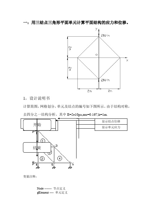
一:用三结点三角形平面单元计算平面结构的应力和位移。
1,设计说明书计算简图,网格划分,单元及结点的编号如下图所示。
由于结构对称,去四分之一结构分析。
其中E=2e10pa,mu=0.167,h=1m.变量注释:Node ------- 节点定义gElement ---- 单元定义gMaterial --- 材料定义,包括弹性模量,泊松比和厚度gBC1 -------- 约束条件gNF --------- 集中力gk------------总刚gDelta-------结点位移子程序注释:PlaneStructualModel ———定义有限元模型SolveModel ———————求解有限元模型DisplayResults ——————显示计算结果k = StiffnessMatrix( ie )———计算单元刚度AssembleStiffnessMatrix( ie, k )—形成总刚es = ElementStress( ie )————计算单元应力function exam1% 输入参数:无% 输出结果:节点位移和单元应力PlaneStructualModel ; % 定义有限元模型SolveModel ; % 求解有限元模型DisplayResults ; % 显示计算结果return ;function PlaneStructualModel% 定义平面结构的有限元模型% 输入参数:无% 说明:% 该函数定义平面结构的有限元模型数据:% gNode ------- 节点定义% gElement ---- 单元定义% gMaterial --- 材料定义,包括弹性模量,泊松比和厚度% gBC1 -------- 约束条件% gNF --------- 集中力global gNode gElement gMaterial gBC1 gNF% 节点坐标% x ygNode = [0.0, 2.0 % 节点10.0, 1.0 % 节点21.0, 1.0 % 节点30.0, 0.0 % 节点41.0, 0.0 % 节点52.0, 0.0] ; % 节点6% 单元定义% 节点1 节点2 节点3 材料号gElement = [3, 1, 2, 1 % 单元15, 2, 4, 1 % 单元22, 5, 3, 1 % 单元36, 3, 5, 1]; % 单元4 % 材料性质% 弹性模量泊松比厚度gMaterial = [1e0, 0, 1] ; % 材料1% 第一类约束条件% 节点号自由度号约束值gBC1 = [ 1, 1, 0.02, 1, 0.04, 1, 0.04, 2, 0.05, 2, 0.06, 2, 0.0] ;% 集中力% 节点号自由度号集中力值gNF = [ 1, 2, -1] ;returnfunction SolveModel% 求解有限元模型% 输入参数:无% 说明:% 该函数求解有限元模型,过程如下% 1. 计算单元刚度矩阵,集成整体刚度矩阵% 2. 计算单元的等效节点力,集成整体节点力向量% 3. 处理约束条件,修改整体刚度矩阵和节点力向量% 4. 求解方程组,得到整体节点位移向量global gNode gElement gMaterial gBC1 gNF gK gDelta% step1. 定义整体刚度矩阵和节点力向量[node_number,dummy] = size( gNode ) ;gK = sparse( node_number * 2, node_number * 2 ) ;f = sparse( node_number * 2, 1 ) ;% step2. 计算单元刚度矩阵,并集成到整体刚度矩阵中[element_number,dummy] = size( gElement ) ;for ie=1:1:element_numberk = StiffnessMatrix( ie ) ;AssembleStiffnessMatrix( ie, k ) ;end% step3. 把集中力直接集成到整体节点力向量中[nf_number, dummy] = size( gNF ) ;for inf=1:1:nf_numbern = gNF( inf, 1 ) ;d = gNF( inf, 2 ) ;f( (n-1)*2 + d ) = gNF( inf, 3 ) ;end% step4. 处理约束条件,修改刚度矩阵和节点力向量。
一 三节点三角形单元
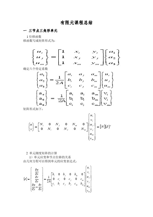
有限元课程总结一 三节点三角形单元 1位移函数移函数写成矩阵形式为:确定六个待定系数矩阵形式如下:[]{}em m j j i i m jim j iN v u v u v u N N N N N N v u δ=⎪⎪⎪⎪⎭⎪⎪⎪⎪⎬⎫⎪⎪⎪⎪⎩⎪⎪⎪⎪⎨⎧⎥⎦⎤⎢⎣⎡=⎭⎬⎫⎩⎨⎧000002 单元刚度矩阵的计算1)单元应变和节点位移的关系由几何方程可以得到单元的应变表达式,{}⎪⎪⎪⎪⎭⎪⎪⎪⎪⎬⎫⎪⎪⎪⎪⎩⎪⎪⎪⎪⎨⎧⎥⎥⎥⎦⎤⎢⎢⎢⎣⎡=⎪⎪⎪⎭⎪⎪⎪⎬⎫⎪⎪⎪⎩⎪⎪⎪⎨⎧∂∂+∂∂∂∂∂∂=m m j j i i m mjjiim j i m j i v u v u v u b c b c b c c c c b b b A x v y u y v x u 00000021ε⎪⎭⎪⎬⎫⎪⎩⎪⎨⎧⎥⎥⎥⎦⎤⎢⎢⎢⎣⎡=⎪⎭⎪⎬⎫⎪⎩⎪⎨⎧321111a a a y x y x y x u u u m m j j i i m j i ⎪⎭⎪⎬⎫⎪⎩⎪⎨⎧⎥⎥⎥⎦⎤⎢⎢⎢⎣⎡=⎪⎭⎪⎬⎫⎪⎩⎪⎨⎧m j i m j i m j i m j i u u u c c c b b b a a a A a a a 21321⎪⎭⎪⎬⎫⎪⎩⎪⎨⎧⎥⎥⎥⎦⎤⎢⎢⎢⎣⎡=⎪⎭⎪⎬⎫⎪⎩⎪⎨⎧m j i m j i m jim ji 654v v v c c c b b b a a a A 21a a a2)单元应力与单元节点位移的关系[][][]⎥⎥⎥⎥⎥⎦⎤⎢⎢⎢⎢⎢⎣⎡---==i i i i i ii i b c c b c b A E B D S 2121)1(22μμμμμ),,;,,(21212121)1(4]][[][][2m j i s m j i r b b c c cb bc b c c b c c b b A Et B D B K s r s r sr s r s r s r s r s r s T r rs ==⎥⎥⎥⎦⎤⎢⎢⎢⎣⎡-+-+-+-+-==μμμμμμμ3)单元刚度矩阵[][][][][][]Tm j iT m T j T i mm mj mi jm jj ji im ij ii e B B B D B B B tA K K K K K K K K K K ⎪⎭⎪⎬⎫⎪⎩⎪⎨⎧=⎥⎥⎥⎦⎤⎢⎢⎢⎣⎡=][][][][][][][][][3载荷移置1)集中力的移置如图3所示,在单元内任意一点作用集中力 {}⎭⎬⎫⎩⎨⎧=y x P P P图3由虚功相等可得,()()}{][}{}{}{**P N R TTe eTe δδ=由于虚位移是任意的,则 }{][}{P N R Te =2)体力的移置令单元所受的均匀分布体力为⎭⎬⎫⎩⎨⎧=y x p ρρ}{由虚功相等可得,()()⎰⎰=tdxdy p N R T TeTe }{][}{}{}{**δδ⎰⎰=tdxdy p N R T e }{][}{ 3)分布面力的移置设在单元的边上分布有面力{}TY X P ],[=,同样可以得到结点载荷,⎰=s T e tdsP N R }{][}{4. 引入约束条件,修改刚度方程并求解1)乘大数法处理边界条件图3-4所示的结构的约束和载荷情况,如图3-7所示。
有限元课程问题汇总(完整版)(1)
1、有限元方法与传统力学方法的比较,有限元的一般概念及基本思路。
叙述有限元方法的基本步骤。
答:比较:运用有限元方法解决工程实际问题时,不管是简单结构或者是复杂的结构,其求解过程是完全相同的,由于每个步骤都具有标准化和规范性的特征,可以在计算机上进行编程而自行实现,这是常规解析方法无法实现的。
即技术核心所在就是采用分段离散的方式来组合出全场几何域上的试函数,而不是直接寻找全场上的试函数。
概念:有限元方法是求解各种复杂数学物理问题的重要方法,是处理各种复杂工程问题的重要分析手段,也是进行科学研究的重要工具。
该方法的应用和实施包括三个方面:计算原理、计算机软件、计算机硬件。
有限元方法的基本思路:将连续系统分割成有限个分区或单元,对每个单元提出一个近似解,再将所有单元按标准方法组合成一个与原有系统近似的系统。
(在具备大规模计算能力的前提下,将复杂的几何物体等效离散为一系列的标准形状几何体,再在标准的几何体上研究规范化的试函数表达及其全场试函数的构建,然后利用最小势能原理建立起力学问题的线性方程组。
)有限单元法解题步骤:①结构的离散化,即单元网格划分;②选择位移模式;③分析单元的力学特征,利用几何方程导出结点位移表示的单元应变,利用本构方程建立单元内任意一点的应力与应变的关系,利用变分原理建立单元的平衡方程;④集合所有单元的平衡方程,建立整个结构的平衡方程(即总的平衡方程),包括将刚度集成总刚,以及将单元的等效结点力列阵集成总的荷载列阵;⑤求解结点位移和计算单元应力,包括边界条件修正;⑥解方程,得到未知问题的节点值;⑦后处理。
2、掌握位移函数和形函数的概念,掌握二者之间的关系。
答:位移函数:是单元内部位移变化的数学表达式,设为坐标的函数,由于有限元法采用能量原理进行单元分析,因而必须事先设定位移函数。
在弹性力学中,恰当选取位移函数不是一件容易的事情;但在有限元中,当单元划分得足够小时,把位移函数设定为简单的多项式就可以获得相当好的精确度。
现代设计方法4-3 三角形三节点平面单元

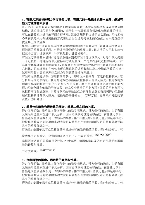
y x y x 1− 0 1− 0 (−1+ + ) 0 b ΙΙ a b a [N] = x y x y 0 1− 0 1− 0 (−1+ + ) b a b a
将a=1, b=2m代入上式得:
x x 0 1− y 0 −1+ + y 0 1− 2 ΙΙ 2 [N] = x x 0 1− 0 1− y 0 −1+ + y 2 2
单元Ⅱ如图所示∆=ab/2。 ④求常数
ai = xi ym − xm y j = ab a = x y − x y = ab m i i m j am = xi y j − xj yi = −ab bi = y j − ym = −a bj = ym − yi = 0 bm = yi − y j = a ci = xm − xj = 0 cj = xi − xm = −b c = x − x = b j i m
作业:
已知三角形三节点单元坐标如图示,设单元中一点A的 坐标(0.5,0.2),已知三角形三节点单元i节点位移(2.0,1.0), j节点位移(2.1,1.1), m节点位移(2.15,1.05), 1)写出单元的位移函数;2)求A点的位移分量。 y j(1,1)
x m(0,0) i(1,0)
2.2 由节点位移求单元的应变
m
三角形三节点单元
六个位移分量需六个待定参数
α1,α2 L α6 L
设单元位移分量是坐标x,y的线性函数,即:
u(x, y) = α1 +α2 x +α3 y v(x, y) = α4 +α5x +α6 y
写成矩阵的形式为:
(1)
平面三角形3节点有限元程序

平面三角形3结点有限元程序1、程序名:,2、程序功能本程序能计算弹性力学的平面应力问题和平面应变问题;能考虑自重和结点集中力两种荷载的作用,在计算自重时y轴取垂直向上为正;能处理非零已知位移,如支座沉降的作用。
主要输出的内容包括:结点位移、单元应力、主应力、第一主应力与x轴的夹角以及约束结点的支座反力。
程序采用Visual Fortran 编制而成,输入数据全部采用自由格式。
3、程序流程及框图图1-1 程序流程图图1-2 程序框图其中,各子程序的功能如下:INPUT——输入结点坐标、单元信息和材料参数;MR——形成结点自由度序号矩阵;FORMMA——形成指标矩阵MA(N)并调用其他功能子程序,相当于主控程序;DIV——取出单元的3个结点号码和该单元的材料号并计算单元的b i,c i等;MGK——形成整体劲度矩阵并按一维存放在SK(NH)中;LOAD——形成整体结点荷载列阵F;OUTPUT——输出结点位移或结点荷载;TREAT——由于有非零已知位移,对K和F进行处理;DECOMP——整体劲度矩阵的分解运算;FOBA——前代、回代求出未知结点位移δ;ERFAC——计算约束结点的支座反力;KRS——计算单元劲度矩阵中的子块K rs。
4、输入数据及变量说明当程序开始运行时,按屏幕提示,键入数据文件的名字。
在运行程序之前,必须根据程序中输入要求建立一个存放原始数据的文件,这个文件的名字由少于8个字符或数字组成。
数据文件包括如下内容:⑴总控信息,共一条,9个数据NP,NE,NM,NR,NI,NL,NG,ND,NCNP——结点总数;NE——单元总数;NM——材料类型总数;NR——约束结点总数;NI ——问题类型标识,0为平面应力问题,1为平面应变问题;NL ——受荷载作用的结点的数目;NG ——考虑自重作用为1,不计自重为0;ND ——非零已知位移结点的数目;NC ——要计算支座约束反力的结点数目。
⑵ 材料信息,共NM 条,每条依次输入EO ,VO ,W ,tEO ——弹性模量(kN/m 2);VO ——泊松比;W ——材料容重(kN/m 3);t ——单元厚度(m )。
- 1、下载文档前请自行甄别文档内容的完整性,平台不提供额外的编辑、内容补充、找答案等附加服务。
- 2、"仅部分预览"的文档,不可在线预览部分如存在完整性等问题,可反馈申请退款(可完整预览的文档不适用该条件!)。
- 3、如文档侵犯您的权益,请联系客服反馈,我们会尽快为您处理(人工客服工作时间:9:00-18:30)。
0 ai
cj 0
0 aj
cm 0
0
am
0
bi
0 bj
0
bm
0 ci 0 c j 0 cm
Ni
(x, 0
y)
0 Ni (x, y)
N j (x, y) 0
0 N j (x, y)
Nm(x, y) 0
0
Nm
(
x,
y)
[N(x, y)]
Ni
(x,
y)
1 2
(ai
bi
x
ci
y)
ijm
d
(
a1
1 A
ui uj um
其中,
xi xj
yi yj
1
a2
1 A
1
ui uj
xm ym
1 um
1 xi yi A 1 xj yj
1 xm ym
yi yj
1
a3
1 A
1
xi xj
ym
1 xm
ui uj um (b)
对v同理可列出a4、a5、a6的方程 :
vi = a4+a5 xi+a6 yi
0
ci
0 cj
0
cm
由单元节点位移{d }e求单元内部任一点位移{d (x,y)}
{d (x,y)}=[m(x,y)]{a }=[m(x,y)][L]{d }e
ai 0 a j 0 am 0
bi
0 bj
0 bm
0
[m(
x,
y)][L]
1 0
x 0
y 0
0 1
0 x
0 y
1 2
ci 0
单元分析的步骤:
节点 (1) 单元内部 (2) 单元 (3) 单元 (4) 节点
位移
各点位移
应变
应力
力
单元分析
2.1 由节点位移求单元内部任一点位移
(1) 单元位移模式
有限元法中,通常采用位移法进行计算,即取节点的位移分量
为基本未知量,单元中的位移、应变、应力等物理量,都和基
本未知量相关联。
y
节点i的位移分量可写成
三角形单元i, j, m在ij边上的形函数与第三个顶点 的坐标无关。
例:求图示单元Ⅰ和单元Ⅱ的形函数矩阵
y
4
ji
Ⅰ
m
1
P/2
3
m
Ⅱ
ij
x
2
P/2
y j (0, a)
y
(0, a)
i
Ⅱ
a
Ⅰ
b
m
(0, 0)
(a)
ix
(b)
(b,0)
分别如上图所示:
Ni
(x,
y)
1 2
(ai
bi x
ci
y)
ijm
(b, a)
x,
y
)
u(x, v(x,
y) y)
N
(
x,
y)d
e
u(x, y) Ni (x, y)ui N j (x, y)u j Nm (x, y)um
v(x,
y)
Ni
(x,
y)vi
N
j
(x,
y)v j
Nm
(x,
y)vm
Ni, Nj, Nm是坐标的连续函数,反映单元内位移的分布 状态,称为位移的形状函数,简称形函数(shape
解出a1~ a6结果:
a1
1 2
(aiui
a ju
j
amum
)
a2
1 2
(biui
bju j
bmum )
a3
1 2
(ciui
c ju j
cmum
)
a
4
1 2
(aivi
ajvj
amvm
)
a5
1 2
(bivi
bjvj
bmvm )
a6
1 2
(civi
cjvj
cmvm )
{a }=[L]{d }e
为三角形单元面积。
m
jx
(b,0)
①单元Ⅰ如图所示。设a=1m, b=2m.
1
1
2 (xi y j xj yi xm yi xi ym xj ym xm y j ) 2 ab
(或直接由图形可知其面积)
②求系数ai, aj, am, bi, bj, bm, ci, cj, cm
y j (0, a)
function)。矩阵[N]称为形函数矩阵(shape function
matrix) 。
➢形函数物理意义:Ni(x,y) ,节点i单位位移,其它节点 位移分量为0,单元内部产生位移分布形状
形函数的性质:
在单元任一点上,三个形函数之和等于1。 形函数Ni在i点的函数值为1,在j点及m点的
函数值为零。
i, j, m
解得: a4、a5、a6
为了书写的简便与规格化,引入记号
ai
xj xm
yj ym
x j ym xm y j
bi
1
1
yj ym
y j ym
1 ci 1
xj xm
xm x j
ijm
1 xi yi A 1 xj yj
1 xm ym
ai, bi, ci分别为行列式A中各行各个元素的代数余子式
u(x, v(x,
y) y)
a1 a4
a2 a5
x x
a3 a6
y y
(4.22)
写成矩阵的形式为:
a1
a
2
d
(x,
y)
u(x, v(x,
y)
y)
1 0
x 0
y 0
0 1
0 x
0
y
a a
3 4
m(
x,
y)a
a
5
a6
(4.23)
(2) 由单元节点位移{d }e求位移参数{a }
a
Ⅰ
b
m
(0, 0)
ix
(b,0)
Ni (x,
y)
1 2
(ai
bi x
ci
y)
ijm
ai x j ym xm y j 0 a j xm yi xi ym 0
am xi y j x j yi ab
bbij
y j ym ym y j
a 0
bm yi y j a
设节点i,j,m坐标分别是xi,yi;xj,yj;xm,ym。把三个节点 的坐标及其水平位移代入式(4.22)中得:
uuij
a1 a1
a2 xi a2x
a3 yi j a3y
j
解得:um a1 a2 xm a3 ym
uuij
1 1
xi xj
yi yj
aa12
(a)
um 1 xm ym a3
1 2
1 A 11
2
xi xj
yi yj
1 xm ym
1 2
(x
j
ym
yj
xi
ym
xj
yi
)
将a写成矩阵形式,有{a }=[L]{d }e
ai 0 a j 0 am 0
bi
0 bj
0 bm
0
L
1 2
ci
0
0 ai
cj 0
0 aj
cm 0
0
am
0 bi 0 bj 0 bm
vj
j
uj
{di} = [ui vi]T
单元节点位移向量{d }e可写成
{d }e = [di dj dm]T
= [ui vi uj vi um vm]T
v
vm
u
m
um
三角形三节点单元
vi ui
i
x
六个位移分量需六个待定参数
a1,a2,……,a6
设单元内任一点位移分量是坐标(x,y)的线性函数:
4.3 平面问题的有限单元法
三角形三节点平面单元
有限元分析的基本步骤:
结构离散化
单元分析
整体分析
1 结构离散化
1m
例:图示一悬臂梁,梁的厚度为t,设泊松比m =1/3,
弹性模量为E,试用三节点三角形单元进行离散。
P/2
A
P/2 y
4
3
2m
l
ji
m
Ⅱ
P/2
Ⅰ
m
ij
x
1
2
P/2
2 单元分析
单元分析的主要内容:由节点位移求内部任一点的 位移,由节点位移求单元应变、应力和节点力。