并行化的krylov子空间方法
Krylov子空间方法II
max {q (λi )2 }
2 yi λi
min
max {q (λi ) } y Λy
5/76
= = 即
q ∈Pk , q (0)=1 1≤i≤n q ∈Pk , q (0)=1 1≤i≤n
min
max {q (λi )2 } ϵ0 Aϵ0 max {q (λi )2 } ∥ϵ0 ∥2 A,
⊺
min
11/76
(4.6)
又 Λ 是对角矩阵, 所以 ∥q (Λ)∥2 = max |q (λi )|.
1≤i≤n
设 x(k) 是由 GMRES 方法得到的近似解. 由 GMRES 方法的最优性可 知, x(k) 极小化残量的 2 范数. 因此, ∥b − Ax(k) ∥2 = = ≤
x∈x(0) +Kk (A,r0 ) q ∈Pk , q (0)=1 q ∈Pk , q (0)=1
1+ε δ
10/76
5.2 GMRES 方法的收敛性
正规矩阵情形 设 A 是正规矩阵, 即 A = U ΛU ∗ , 其中 Λ = diag(λ1 , λ2 , . . . , λn ) 的对角线元素 λi ∈ C 为 A 的特征值. 设 x ∈ x(0) + Kk (A, r0 ), 则存在多项式 p(t) ∈ Pk−1 使得 x = x(0) + p(A)r0 . 于是 b − Ax = b − Ax(0) − Ap(A)r0 = (I − Ap(A))r0 ≜ q (A)r0 , 其中 q (t) = 1 − t p(t) ∈ Pk 满足 q (0) = 1. 直接计算可知 ∥b − Ax∥2 = ∥q (A)r0 ∥2 = ∥U q (Λ)U ∗ r0 ∥2 ≤ ∥U ∥2 ∥U ∗ ∥2 ∥q (Λ)∥2 ∥r0 ∥2 = ∥q (Λ)∥2 ∥r0 ∥2 .
预处理子空间迭代法的一些基本概念
CG算法的预处理技术:、为什么要对A进行预处理:其收敛速度依赖于对称正定阵A的特征值分布特征值如何影响收敛性:特征值分布在较小的范围内,从而加速CG的收敛性特征值和特征向量的定义是什么?(见笔记本以及收藏的网页)求解特征值和特征向量的方法:Davidson方法:Davidson 方法是用矩阵( D - θI)- 1( A - θI) 产生子空间,这里D 是A 的对角元所组成的对角矩阵。
θ是由Rayleigh-Ritz 过程所得到的A的近似特征值。
什么是子空间法:Krylov子空间叠代法是用来求解形如Ax=b 的方程,A是一个n*n 的矩阵,当n充分大时,直接计算变得非常困难,而Krylov方法则巧妙地将其变为Kxi+1=Kxi+b-Axi 的迭代形式来求解。
这里的K(来源于作者俄国人Nikolai Krylov姓氏的首字母)是一个构造出来的接近于A的矩阵,而迭代形式的算法的妙处在于,它将复杂问题化简为阶段性的易于计算的子步骤。
如何取正定矩阵Mk为:Span是什么?:设x_(1,)...,x_m∈V ,称它们的线性组合∑_(i=1)^m?〖k_i x_i \|k_i∈K,i=1,2...m〗为向量x_(1,)...,x_m的生成子空间,也称为由x_(1,)...,x_m张成的子空间。
记为L(x_(1,)...,x_m),也可以记为Span(x_(1,)...,x_m)什么是Jacobi迭代法:什么是G_S迭代法:请见PPT《迭代法求解线性方程组》什么是SOR迭代法:什么是收敛速度:什么是可约矩阵与不可约矩阵?:不可约矩阵(irreducible matrix)和可约矩阵(reducible matrix)两个相对的概念。
定义1:对于n 阶方阵A 而言,如果存在一个排列阵P 使得P'AP 为一个分块上三角阵,我们就称矩阵A 是可约的;否则称矩阵A 是不可约的。
定义2:对于n 阶方阵A=(aij) 而言,如果指标集{1,2,...,n} 能够被划分成两个不相交的非空指标集J 和K,使得对任意的j∈J 和任意的k∈K 都有ajk=0, 则称矩阵 A 是可约的;否则称矩阵A 是不可约的。
Krylov子空间方法

由于 x ˜ ∈ x(0) + K, 因此存在向量 y ∈ Rm 使得 x ˜ = x(0) + V y 由正交性条件 (4.4) 可知 r0 − AV y ⊥ wi , i = 1, 2, . . . , m , 即 W ⊺ AV y = W ⊺ r0 .
x ˆ≜x ˜ − x(0) = V y
9/115
Arnoldi 过程: 计算 Km 的一组正交基
算法 2.1 基于 Gram-Schmidt 正交化的 Arnoldi 过程
1: 2: 3: 4: 5: 6: 7: 8: 9: 10: 11: 12: 13:
给定非零向量 r, 计算 v1 = r/∥r∥2 for j = 1, 2, . . . , m − 1 do wj = Avj for i = 1, 2, . . . , j do hij = (wj , vi ) end for j ∑ wj = wj − hij vi hj +1,j = ∥wj ∥2 if hj +1,j = 0 then break end if vj +1 = wj /hj +1,j end for
若给定初值 x(0) ∈ Rn , 则改用仿射空间 x(0) + K, 即 find x ˜ ∈ x(0) + K such that b − Ax ˜ ⊥ L. (4.3)
好的初值一般都包含有价值 的信息
事实上, 如果将 x ˜ 写成: x ˜ = x(0) + x ˆ, 其中 x ˆ ∈ K, 则 (4.3) 就等价于 find x ˆ∈K such that r0 − Ax ˆ ⊥ L, (4.4)
定解条件
r = b − Ax ˜⊥L 其中 x ˜ 是近似解, L 是另一个 m 维子空间. 不同的 L 对应不同的投影方法 当 L = K 时, 我们称为 正交投影法 , 否则称为 斜投影法
Krylov子空间迭代法

采用IOM后,仍然需要存储v(1), v(2), …v(m),因为在第(vi)步 中仍然需要这些向量. 解决这个问题可以考虑采用H的LU分解,通过自身分解的迭代更新以减少每 一步的存储量 使xm的更新依赖于xm-1,
14
Arnoldi方法-DIOM
lower bidiagonal
banded upper triangular
15
Arnoldi方法-DIOM
16
Arnoldi方法-DIOM
17
Thanks for your time !
18
得到基于Galerkin原 理构成的算法
5
Arnoldi方法-基本算法
6
Arnoldi方法-基本算法
7
Arnoldi方法-MGS
8
Arnoldi方法-HO
9
Arnoldi方法-FOM
10
Arnoldi方法-FOM
11
Arnoldi方法-FOM(m)
12
Arnoldi方法-IOM
13
Arnoldi方法-DIOM
Krylov子空间方法
March 23, 2016
内
• Arnoldi算法
– Arnoldi过程 – Gram-Schmidt Arnoldi – HouseHolder Arnoldi
容
• 子空间和Krylov子空间
• FOM
– IOM – DIOM
2
子空间
• 空间
– 集合,元素都是向量 – 线性空间(向量空间)
• 线性空间(交换律,结合律,幺元性,零元性,可 逆性,数乘分配律等)
• 子空间
– 线性空间的非空子集
Krylov子空间、优化问题与共轭梯度法
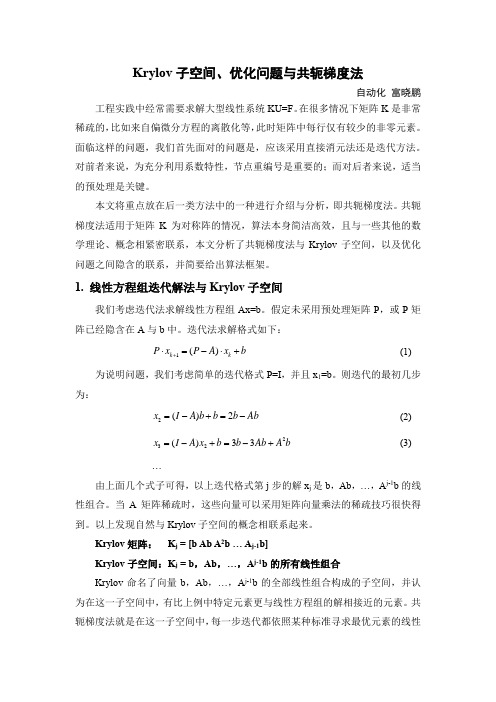
Krylov 子空间、优化问题与共轭梯度法自动化 富晓鹏工程实践中经常需要求解大型线性系统KU=F 。
在很多情况下矩阵K 是非常稀疏的,比如来自偏微分方程的离散化等,此时矩阵中每行仅有较少的非零元素。
面临这样的问题,我们首先面对的问题是,应该采用直接消元法还是迭代方法。
对前者来说,为充分利用系数特性,节点重编号是重要的;而对后者来说,适当的预处理是关键。
本文将重点放在后一类方法中的一种进行介绍与分析,即共轭梯度法。
共轭梯度法适用于矩阵K 为对称阵的情况,算法本身简洁高效,且与一些其他的数学理论、概念相紧密联系,本文分析了共轭梯度法与Krylov 子空间,以及优化问题之间隐含的联系,并简要给出算法框架。
1. 线性方程组迭代解法与Krylov 子空间我们考虑迭代法求解线性方程组Ax=b 。
假定未采用预处理矩阵P ,或P 矩阵已经隐含在A 与b 中。
迭代法求解格式如下:1()k k P x P A x b +⋅=-⋅+ (1)为说明问题,我们考虑简单的迭代格式P=I ,并且x 1=b 。
则迭代的最初几步为:2()2x I A b b b Ab =-+=- (2)232()33x I A x b b Ab A b =-+=-+ (3) …由上面几个式子可得,以上迭代格式第j 步的解x j 是b ,Ab ,…,A j -1b 的线性组合。
当A 矩阵稀疏时,这些向量可以采用矩阵向量乘法的稀疏技巧很快得到。
以上发现自然与Krylov 子空间的概念相联系起来。
Krylov 矩阵: K j = [b Ab A 2b … A j -1b]Krylov 子空间:K j = b ,Ab ,…,A j -1b 的所有线性组合Krylov 命名了向量b ,Ab ,…,A j -1b 的全部线性组合构成的子空间,并认为在这一子空间中,有比上例中特定元素更与线性方程组的解相接近的元素。
共轭梯度法就是在这一子空间中,每一步迭代都依照某种标准寻求最优元素的线性方程组解法。
krylov子空间算法

Krylov 子空间的定义:定义:令N R υ∈,由1m A υυυ-,,,A 所生成的子空间称之为由υ与A 所生成的m 维Krylov 子空间,并记(),m K A v 。
主要思想是为各迭代步递归地造残差向量,即第n 步的残差向量()n r 通过系数矩阵A 的某个多项式与第一个残差向量()0r 相乘得到。
即()()()0n r p A r =。
但要注意,迭代多项式的选取应该使所构造的残差向量在某种内积意义下相互正交,从而保证某种极小性(极小残差性),达到快速收敛的目的。
Krylov 子空间方法具有两个特征:1.极小残差性,以保证收敛速度快。
2.每一迭代的计算量与存储量较少,以保证计算的高效性。
投影方法线性方程组的投影方法方程组Ax b =,A 是n n ⨯的矩阵。
给定初始()0x ,在m 维空间K(右子空间)中寻找x 的近似解()1x 满足残向量()1r b Ax =-与m 维空间L(左子空间)正交,即()1b Ax L -⊥,此条件称为Petrov-Galerkin 条件。
当空间K=L 时,称相应的投影法为正交投影法,否则称为斜交投影法.投影方法的最优性:1. (误差投影)设A 为对称正定矩阵,()0x 为初始近似解,且K=L,则()1x 为采用投影方法得到的新近似解的充要条件是()()()()01min z x Kx z ϕϕ∈+=其中,()()()12,z A x z x z ϕ=--2.(残量投影)设A 为任意方阵,()0x 为初始近似解,且L AK =,则()1x 为采用投影方法得到的新近似解的充要条件是()()()()01min z x Kx z ψψ∈+=其中()()122,z b Az b Az b Az ψ=-=--矩阵特征值的投影方法对于特征值问题Ax x λ=,其中A 是n ×n 的矩阵,斜交投影法是在m 维右子空间K 中寻找i x 和复数i λ满足i i i Ax x L λ-⊥,其中L 为m 维左子空间.当L=K 时,称此投影方法为正交投影法. 误差投影型方法: 取L=K 的正交投影法非对称矩阵的FOM 方法(完全正交法) 对称矩阵的IOM 方法和DIOM 方法 对称矩阵的Lanczos 方法 对称正定矩阵的CG 方法 残量投影型方法: 取L=AK 时的斜交投影法GMERS 方法(广义最小残量法) 重启型GMERS 方法、QGMERS 、DGMERSArnoldi 方法标准正交基方法:Arnoldi 方法是求解非对称矩阵的一种正交投影方法。
(完整版)Krylov子空间迭代法
February 10, 2020
内容
• 子空间和Krylov子空间
• Arnoldi算法
– Arnoldi过程 – Gram-Schmidt Arnoldi – HouseHolder Arnoldi
• FOM
– IOM – DIOM
2
子空间
• 空间
– 集合,元素都是向量 – 线性空间(向量空间)
根据Cayley-Hamilton定理有
������������ + ������������−1������������−1+. . . +������1������1 + ������0������0 = 0
即
VP= -������������ 其中������ = [������0, ������1, . . . , ������������−1ሿ,������ = ������0, ������1, . . . , ������������−1 ������ Krylov子空间: ������������(������, ������) = ������������������������{������, ������������, . . . , ������������−1������ሽ Krylov矩阵: ������������(������, ������) = [������, ������������, . . . , ������������−1������ሿ
• 线性空间(交换律,结合律,幺元性,零元性,可 逆性,数乘分配律等)
• 子空间
– 线性空间的非空子集
• 包含零元素,并且满足加法和乘法的封闭性
– 扩张(符合记作span)
第四讲Krylov子空间方法(II)
设 A 对称正定 .
令 x(k) 是 CG 方法在仿射空间 x(0) + Kk(A, r0) 中找到的近似解. 则由 CG 方法的最优性质可知
∥x(k) − x∗∥A =
min
∥x − x∗∥A
x∈x(0) +Kk (A,r0 )
(4.1)
记 Pk 为所有次数不超过 k 的实系数多项式集合. 则 Kk(A, r0) 中任何 一个向量都可以写成 p(A)r0 形式, 其中 p ∈ Pk−1. 设 x ∈ x(0) + Kk(A, r0), 则存在多项式 p(t) ∈ Pk−1 使得
i=1
yi2λiq(λi)2
∑n
≤
min
q∈Pk, q(0)=1
max {q(λi)2}
1≤i≤n
i=1
yi2λi
= min max {q(λi)2} y⊺Λy q∈Pk, q(0)=1 1≤i≤n
5/76
=
min
q∈Pk, q(0)=1
max {q(λi)2}
1≤i≤n
ϵ⊺0 Aϵ0
=
min
q∈Pk, q(0)=1
≤
min
q∈Pk, q(0)=1
max |q(λi)|.
1≤i≤n
(4.3)
需要指出的是, (4.3) 中上界是紧凑的, 即对任意 k, 总存在某个右端项 b 或某个初始值 x(0) (与 k 和 A 有关), 使得 (4.3) 中的等号成立. 也就是 说, (4.3) 中的上界描述了 CG 方法在最坏情况下的收敛情况.
x = x(0) + p(A)r0.
3/76
记 ϵ0 ≜ x(0) − x∗, 则
x − x∗ = x(0) + qk(A)r0 − x∗ = ϵ0 + p(A)(b − Ax(0)) = ϵ0 + p(A)(Ax∗ − Ax(0)) = (I − Ap(A))ϵ0.
第四讲Krylov子空间方法
如果没有特别注明, 本章内容都是在实数域中讨论.
4.1 投影方法
设 K 是 Rn 的一个子空间, 维数为 dim(K) = m ≪ n. 我们需要在 K 中寻找精确解的一 个 “最佳” 近似. 由于 K 的维数是 m, 为了能够唯一确定这个近似解, 我们需要设置 m 个约 束. 在通常情况下, 我们要求残量满足 m 个正交性条件:
x˜ = x(0) + V y.
· 4-2 ·
由正交性条件 (4.5) 可知 r0 − AV y ⊥ wi, i = 1, 2, . . . , m,
即 W AV y = W r0.
如果 W AV 是非奇异的, 则可解得 y = (W AV )−1W r0. 因此, 近似解 x˜ 可表示为 x˜ = x(0) + V (W AV )−1W r0.
vj+1 = wj /hj+1,j
14: end for
如果计算到第 k (k < m) 步时有 hk+1,k = 0, 则方法会提前终止. 此时 Avk 必定可以由 v1, v2, . . . , vk 线性表出 (这里不考虑浮点运算的舍入误差).
算法 4.1 中的向量 vi 称为 Arnoldi 向量. 需要注意的是, 在该算法中, 我们是用 A 乘以 vj, 然后与之前的 Arnoldi 向量正交化, 而不是计算 Ajr. 事实上, 它们是等价的.
r = b − Ax˜ ⊥ L,
(4.2)
其中 x˜ 是我们所要寻找的近似解, L 是另一个 m 维子空间. 这就是数值计算中常用的 PetrovGalerkin 条件. 如果 L = K, 则称为 Galerkin 条件. 子空间 L 也称为 约束空间 (constraint subspace). 相应地, K 通常称为 搜索空间.
krylov子空间算法
Krylov 子空间的定义:定义:令N R υ∈,由1m A υυυ-L ,,,A 所生成的子空间称之为由υ与A 所生成的m 维Krylov 子空间,并记(),m K A v 。
主要思想就是为各迭代步递归地造残差向量,即第n 步的残差向量()n r 通过系数矩阵A 的某个多项式与第一个残差向量()0r 相乘得到。
即()()()0n r p A r =。
但要注意,迭代多项式的选取应该使所构造的残差向量在某种内积意义下相互正交,从而保证某种极小性(极小残差性),达到快速收敛的目的。
Krylov 子空间方法具有两个特征:1、极小残差性,以保证收敛速度快。
2、每一迭代的计算量与存储量较少,以保证计算的高效性。
投影方法线性方程组的投影方法方程组Ax b =,A 就是n n ⨯的矩阵。
给定初始()0x ,在m 维空间K(右子空间)中寻找x 的近似解()1x 满足残向量()1r b Ax =-与m 维空间L(左子空间)正交,即()1b Ax L -⊥,此条件称为Petrov-Galerkin 条件。
当空间K=L 时,称相应的投影法为正交投影法,否则称为斜交投影法、投影方法的最优性:1、 (误差投影)设A 为对称正定矩阵,()0x 为初始近似解,且K=L,则()1x 为采用投影方法得到的新近似解的充要条件就是()()()()01min z x Kx z ϕϕ∈+=其中,()()()12,z A x z x z ϕ=--2.(残量投影)设A 为任意方阵,()0x 为初始近似解,且L AK =,则()1x 为采用投影方法得到的新近似解的充要条件就是()()()()01min z x Kx z ψψ∈+=其中()()122,z b Az b Az b Az ψ=-=--矩阵特征值的投影方法对于特征值问题Ax x λ=,其中A 就是n ×n 的矩阵,斜交投影法就是在m 维右子空间K 中寻找i x 与复数i λ满足i i i Ax x L λ-⊥,其中L 为m 维左子空间、当L=K 时,称此投影方法为正交投影法、 误差投影型方法: 取L=K 的正交投影法非对称矩阵的FOM 方法(完全正交法) 对称矩阵的IOM 方法与DIOM 方法 对称矩阵的Lanczos 方法 对称正定矩阵的CG 方法 残量投影型方法: 取L=AK 时的斜交投影法 GMERS 方法(广义最小残量法)重启型GMERS 方法、QGMERS 、DGMERSArnoldi 方法标准正交基方法:Arnoldi 方法就是求解非对称矩阵的一种正交投影方法。
- 1、下载文档前请自行甄别文档内容的完整性,平台不提供额外的编辑、内容补充、找答案等附加服务。
- 2、"仅部分预览"的文档,不可在线预览部分如存在完整性等问题,可反馈申请退款(可完整预览的文档不适用该条件!)。
- 3、如文档侵犯您的权益,请联系客服反馈,我们会尽快为您处理(人工客服工作时间:9:00-18:30)。
Article history: Received 3 July 2007 Received in revised form 15 December 2007 Keywords: Sparse nonsymmetric linear system IBiCGSTAB(2) method Krylov subspace method Distributed parallel environments Global communication
1. Introduction Among iterative methods for large sparse systems, Krylov subspace methods are the most powerful. The conjugate gradient (CG) method for solving symmetric positive definite linear systems, the GMRES method, BiCG method [9], QMR method [3], BiCGSTAB method [14], BiCR method [11] and BiCRSTAB method [7] for solving nonsymmetric linear systems and so on are all examples. The basic time-consuming computational kernels of all Krylov subspace methods are usually [9]: inner products, vector updates and matrix-vector multiplications. In many situations, especially when matrix operations are well structured, these operations are suitable for implementation on vector and shared memory parallel computers. But for parallel distributed memory machines, the matrices and vectors are distributed over the processors, so that even when matrix operations can be implemented efficiently by parallel operation, we still cannot avoid the global communication required for inner product computations, i.e. accumulation of data from all the processors to one, and broadcasting the result to each processor. Vector updates are naturally parallel and, for large sparse matrices, matrix-vector multiplications can be implemented with communication only between nearby processors. The bottleneck is usually due to inner products enforcing global communication. These global communication costs become relatively more and more important when the number of
0377-0427/$ – see front matter © 2008 Elsevier B.V. All rights reserved. doi:10.1016/j.cam.2008.05.017
56
T.-X. Gu et al. / Journal of Computational and Applied Mathematics 226 (2009) 55–65
Journal of Computational and Applied Mathematics 226 (2009) 55–65
Contents lists available at ScienceDirect
Journal of Computational and Applied Mathematics
parallel processors is increased and thus they have the potential to affect the scalability of the algorithm in a negative way. A detailed discussion on the communication problem on distributed memory systems can be found in [12,13]. Three remedies can be used to solve the bottleneck which leads to performance degeneration. The first remedy is to eliminate data relativity or reduce the number of global synchronization points, so that several inner products can be computed and passed at the same time. The second is reconstructing the algorithm so that communication and computation can be overlapped efficiently. The last is replacing the inner product computation by other computations which do not require global communications. Of course, they can be used concurrently. Recently, Bücker et al. [1] and Yang et al. [15] proposed a new parallel Quasi-Minimal Residual(QMR) method based on a Lanczos process with coupled two-term recurrence. Sturler et al. [12] proposed how to reduce the effect of global communication in GMRES(m) and CG methods. Yang et al. [16–18] proposed the improved CGS, BiCG and BiCGSTAB methods respectively. Chi et al. gave an improved CR algorithm [2]. Gu, Zuo and Liu et al. [6–8] proposed parallel versions of BiCR, BiCRSTAB and QMRCGSTAB methods. All of these methods depend on the first two strategies. Gu, Liu and Mo [4,5] proposed a CG-type method without global inner products, i.e. multiple search direction conjugate gradient (MSD-CG) method. Based on domain decomposition, the MSD-CG method replaced the inner product computations in the CG method by small size linear systems. Therefore, it eliminates global inner products completely, which belongs to the last remedy. In this paper, we give an improved parallel BiCGSTAB(2) method for distributed parallel environments based on the first two remedies mentioned above. The IBiCGSTAB(2) method is reorganized without changing numerical stability and all inner products per iteration are collected in two steps and independent (only one single global synchronization point), and subsequently communication time required for inner products can be overlapped efficiently with computation time. The cost is only slightly increased computation. Performance and isoefficiency analysis show that the IBiCGSTAB(2) method has better parallelism and scalability than the BiCGSTAB(2) method. Especially, the parallel performance can be improved by a factor greater than 2.5. The paper is organized as follows. In Section 2, the design of the improved parallel BiCGSTAB(2) method is presented. Performance and isoefficiency analysis of the IBiCGSTAB(2) and BiCGSTAB(2) methods are presented in Sections 3 and 4. Numerical experiments carried out on a distributed memory parallel machine are reported in Section 5. Finally, we make some concluding remarks in Section 6. 2. Algorithm design of IBiCGSTAB(2) method Consider solving a large sparse nonsymmetric linear system Ax = b