Microscopic Traffic Flow Simulator VISSIM
基于城市道路网络的动态od估计
2.处理工具
处理工具允许用户用批处理的方式进行仿真计算,并得到统计数据输出。批处理通过图形用户界面来设置仿真参数、选择输出数据和改变车辆特征。用批处理的方式进行交通仿真计算不显示仿真过程车辆的位置和路网。因此大大加快了仿真的速度。处理工具输出的仿真结果与建模工具输出的结果是相同的,但所需的运行时间较少。
作者:何兆成
学位授予单位:中山大学
1.陆化普交通规划理论与方法 1998
2.CASCETTA E Estimation of trip matrices from traffic counts and survey data:A generalized least squares estimator 1984
!
5
;’。≤j毅i≮棚l篓攥惹黪篱ii灞
i…‘‘1。‘‘4。””。‘’1’‘““瞄。m4…‘1。11”。‘’。‘‘一,■8 O
14710131619222528313437404346
时间间隔
图5—6采样周期为300秒时的01]量瓦
估计值与真实值随时间的变化情况
图5·7采样周期为3∞秒时的01]量瓦2
23.NIHAN N.DAVIS G A Recursive estimation of origin-destination matrices from input/output counts 1987
24.NIHAN N L.DAVIS G A Application of prediction-error minimization and maximum likelihood to estimate intersection O-D matrices from traffic counts 1989
VISSIM使用指南
INTRODUCTORY TRAININGVISSIMVISSIM is a microscopic, time step and behavior based simulation model developed to model urban traffic and public transit operations. The program can analyze traffic and transit operations under constraints such as lane configuration, traffic composition, traffic signals, transit stops, etc., thus making it a useful tool for the evaluation of various alternatives based on transportation engineering and planning measures of effectiveness.The traffic simulator in VISSIM is a microscopic traffic flow simulation model including the car following and lane change logic. VISSIM uses the psycho-physical driver behavior model developed by Wiedemann (1974). The basic concept of this model is that the driver of a faster moving vehicle starts to decelerate as he reaches his individual perception threshold to a slower moving vehicle. Since he cannot exactly determine the speed of that vehicle, his speed will fall below that vehicle’s speed until he starts to slightly accelerate again afte r reaching another perception threshold. This results in an iterative process of acceleration and deceleration.Open VISSIM and create a new fileFor every transport network a separate VISSIM file is needed. To create a new network the following steps are to be followed.1.Open the master plan of your study area as a background imageBuilding an accurate VISSIM model at least one scaled map that shows the real network. The image file of a digitized map (.jpg, .tiff, .bmp etc.) is to be imported as a background. This background can be displayed, moved and scaled in the VISSIM network window and is used to trace the VISSIM links and connectors.2.Scale the background and save a scaled background.Precise scaling is necessary for an accurate network model. A large scale distance (> 100 m / > 300 ft) is recommended to use.3. Draw links and connectors for streets and junctionsThe level of detail required for replicating the modeled transport network infrastructure depends on the purpose of a VISSIM application. While a rough outline of the analyzed intersection is sufficient for testing traffic actuated signal logic, a more detailed model is required for simulation analyses.Link: The first step in coding a VISSIM network is to trace links. Each approach and section should be represented by one link. A link cannothave multiple sections with a different number of lanes. Connectors (rather than links) should be used to model turning movements.Connectors: In order to create a road network, links need to be connected to other links. It is not sufficient to place one link on top of another link in order for vehicles to continue on the other link. Instead, a connector needs to be created to connect the two links. Furthermore connectors are used to model turnings of junctions.Set Parameters for the new file1.Simulation ParametersTraffic regulations: Specifies the standard driving side (For Ireland, Leftside-Traffic).Simulation Resolution: The number of times the vehicle’s position will be calculated within one simulated second (range 1 to 10) (more than 3 recommended).Random Seed: This parameter initializes the random number generator. Simulation runs with identical input files and random seeds generate identical results. Using a different random seed includes a stochastic variation of input flow arrival times.2.Speed profilesSome parameters in VISSIM are defined as a distribution rather than a fixed value. Thus the stochastic nature of traffic situations is reflected realistically. Most of the distributions are handled similarly and it is possible to use any kind of empirical or stochastic data for definition.Stochastic distributions of desired speeds are defined for each vehicle type within each traffic composition. The minimum and maximum values for the desired speed distribution are to be entered along with two intermediate points are generally adequate to define an s-shaped distribution.3. Vehicle Acceleration and Deceleration FunctionsVISSIM does not use a single acceleration and deceleration value but uses functions to represent the differences in a driver’s behavior. Acceleration and deceleration are functions of the current speed. These functions are predefined for each of the default vehicle types in VISSIM. They can be edited or new graphs can be created4. Dwell Time Distribution (Stops & Parking Lots)The dwell time distribution is used by VISSIM for dwell times at parking lots, stop signs, toll counters or transit stops. Either a normal distribution or an empirical distribution can be provided for transit stops.5. Vehicle type characteristicsIn addition to the default vehicle types (Car, HGV, Bus, Tram, Bike and Pedestrian), new vehicle types can be created or existing types modified. A vehicle class represents a logical container for one or more previously defined vehicle types.6. Create traffic compositionsA traffic composition defines the vehicle mix of each input flow to be defined for the VISSIM network. The relative percentage (proportion) of each vehicle type is to be given.7. Enter traffic volumes at network endpoints and pedestrian volumes at junctionsIn VISSIM, time variable traffic volumes to enter the network can be defined. For vehicle input definition, at least one traffic composition has to be defined. Traffic volumes are defined for each link and each time interval in vehicles per hour. Within one time interval vehicles enter the link based on a Poisson distribution.Fine Tuning of the VISSIM Network1. Enter routing decision points and associated routesA route is a fixed sequence of links and connectors. A route starts from a routing decision point (red cross-section) and extends up to at least one destination point (green cross-section) or multiple destinations. A route can have any length - from a turning movement at a singlejunction to a route that stretches throughout the entire VISSIM network.For static routing decisions, vehicles from a start point (red) to any of the defined destinations (green) using a static percentage for each destination.2. Enter speed changesReduced speed areas: When modeling short sections of slow speed characteristics (e.g. curves or bends), the use of reduced speed areas is advantageous over the use of desired speed decisions. In order for a reduced speed area to become effective vehicles need to pass its start position.Desired Speed Decisions: A desired speed decision is to be placed at a location where a permanent speed change should become effective. The typical application is the location of a speed sign in reality.3. Enter priority rulesPriority rules are to be applied for non-signalized intersections, permissive left turns, right turns on red light and pedestrian crosswalks. The right-of-way for non-signal-protected conflicting movements is modeled with priority rules. This applies to all situations where vehicles on different links/connectors should recognize each other. The two main conditions to check at the conflict marker(s) are minimum headway (distance) and minimum gap time.Conflict areas are a new alternative to priority rules to define priority in intersections. They are the recommended solution in most casesbecause they are more easily defined and the resulting vehicle behavior is more intelligent. A conflict area can be defined wherever two links/connectors in the VISSIM network overlap. For each conflict area, the user can select which of the conflicting links has right of way (if any).4. Enter stop signsIntersection approaches controlled by STOP signs are modeled in VISSIM as a combination of priority rule and STOP sign. A STOP sign forces vehicles to stop for at least one time step regardless of the presence of conflicting traffic while the priority rule deals with conflicting traffic, looking for minimum gap time and headway etc. STOP signs are required to be installed for non-signalized intersections and for right turns on red light.Create Signal ControlsSignalized intersections can be modeled in VISSIM either using the built-in fixed-time control or an optional external signal state generator. (Our license in Trinity has a fixed time control.)In VISSIM every signal controller (SC) is represented by its individual SC number and signal phase. Signal indications are typically updated at the end of each simulation second.Signal control and signal groups are to be modeled from Signal Control window. In Fixed Time Signal Control VISSIM starts a signal cycle at second 1 and ends with second Cycle time.Setup for output files and run simulationstravel time segmentsUsing Travel Time Measurements mode, a section of the network has to be selected on which the travel time is to be measured.The output format can be configured according to the requirement of the user.delay segmentsBased on travel time sections VISSIM can generate delay data for networks. A delay segment is based on one or more travel time sections. All vehicles that pass these travel time sections are captured by the delay segment. A delay time measurement determines - compared to the ideal travel time (no other vehicles, no signal control) - the mean time delay calculated from all vehicles observed on a single or several link sections.queue countersThe queue counter feature in VISSIM provides as output the average queue length, maximum queue length and the number of vehicle stops within the queue. Queues are counted from the location of the queue counter on the link or connector upstream to the final vehicle that is in queue condition. If the queue backs up onto multiple different approaches the queue counter will record information for all of them and report the longest as the maximum queue length.data collection pointsData collection offers the collection of data on single cross sections.QUICKSTART CHECKLIST1. Open VISSIM and create a new file2. Set the simulation parameters3. Create/edit speed profiles4. Check/edit vehicle type characteristics5. Create traffic compositions6. Open the master plan of your study area as a background image7. Place and scale the background image and save background image file.8. Draw links and connectors for roadways tracks and crosswalks9. Enter traffic volumes at network endpoints and pedestrian volumes at junctions10. Enter routing decision points and associated routes11. Enter speed changes12. Enter priority rules for non-signalized intersections13. Enter stop signs for non-signalized intersections14. Create Signal Controls with signal groups15. Enter signal heads in network16. Enter detectors for intersections controlled by traffic actuated signal control17. Enter stop signs for right turns on red18. Enter priority rules19. Create dwell time distributions and place transit stops in network20. Create transit lines21. Setup for output files22. Run the simulation。
交通规划中几种常用软件

特快、大站快车、票价、换乘优惠、换乘时间、 速 度、频度、运力、费率设置。
(3)公交模型分配 Logit模型、多径路分配 公交子方
式模型
O-D间,利用公交的出行比例取决于出行时间。先决 定不同的交通方式,后决定同一交通方式中的不同线 路。
乘车模型
对同一交通方式中的不同线路的选择,取决于服务频 率。 下车模型 在选择了公交的前提下,决定下车站点。
路段基本属性输入:
·名称、设计速度、流向 ·现状通行能力、现状流量 现状通行能力、流量、设计速度
规划年通行能力、设计速度
现
状
道 路 流 量 / 负 荷 度
现状道路机动车高峰小时负荷现状道路机动车高峰小时流量 度
现状OD反推:
现状路网文件 Seed OD Matrix
现状通行能力、流量、设计速度
现状OD Matrix
TransCAD提供:
功能强大的GIS系统,可完成各种交通规划 任务 为交通规划而开发设计的地图处理工具和可 视化工具
需求预测与分析,经营管理决策的应用模型
距离最短
时间最短
规划软件:TransCAD 预测对象:国家话剧院2010年周边道路流量 主要技术线路: 现状OD反推
小区划分,小区内经济社会指标统计,现状交通数据 (断面 交通量、OD交通量)。
二、交通需求预测:四阶段法、交通流模拟 生成交
通量、发生与吸引交通量、分布交通量、交通方式 划分交通量、交通流分配。
三、方案评价:交通量、负荷度、平均行驶车速、平 均出 行距离、断面OD交通量、……
一、STRADA(JICA System for TRAffic Demand Analysis)
微观交通仿真软件分析与比较
微观交通仿真软件分析比较交通仿真技术是智能技术的一个重要组成部分,是计算机技术在交通工程领域的一个重要应用,它可以动态地、逼真地仿真交通流和交通事故等各种交通现象,复现交通流的时空变化,深入地分析车辆、驾驶员和行人、道路以及交通的特征,有效地进行交通规划、交通组织与管理、交通能源节约与物资运输流量合理化等方面的研究。
同时,交通仿真系统通过虚拟现实技术手段,能够非常直观地表现出路网上车辆的运行情况,对某个位置交通是否拥堵、道路是否畅通、有无出现交通事故、以及出现上述情况时采用什么样的解决方案来疏导交通等,在计算机上经济有效且没有风险的仿真出来。
交通仿真作为仿真科学在交通领域的应用分支,是随着系统仿真的发展而发展起来的。
它以相似原理、信息技术、系统工程和交通工程领域的基本理论和专业技术为基础。
以计算机为主要工具,利用系统仿真模型模拟道路交通系统的运行状态。
采用数字方式或图形方式来描述动态交通系统,以便更好地把握和控制该系统的一门实用技术。
交通相关仿真按类别分为交通流仿真、自动驾驶仿真和交通事故复原仿真等几个类型。
其中交通仿真又按仿真的精确程度和范围分为宏观仿真、中观仿真和微观仿真。
此外交通仿真中有关行人交通流的仿真因为场景不一样又可以单独分离出来单独处理,特别适合于大型公共场所、进出口、通道等的研究。
图0 交通相关仿真分类在众多的交通仿真软件中如何选取最合适的软件作为评价的工具,一般取决于项目的要求和目标而定。
一、主要微观交通仿真软件自20世纪60年代以来,国内外交通业界在微观交通仿真领域进行了卓有成效的研究工作,开发了几十种微观交通仿真模型和多种交通仿真软件系统。
本文将对主要的5种仿真软件进行技术特性分析和性能比较。
(一)VISSIMVISSIM 是德国PTV公司的产品,它是一个离散的、随机的、以100s为时间步长的微观仿真模型。
车辆的纵向运动采用心理- 物理跟驰模型(psycho - physical car –following model ),横向运动(车道变换)则采用基于规则(rule –based)的算法。
Micro-FLO FLOW VERIFICATION SYSTEM (FVS) 使用指南说明书
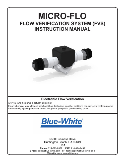
Electronic Flow VerificationAre you sure the pump is actually pumping?Empty chemical tank, clogged injection fitting, lost prime, an other problems can prevent a metering pump from actually injecting chemical - even though the pump is in good working order.MICRO-FLOFLOW VERIFICATION SYSTEM (FVS)INSTRUCTION MANUAL5300 Business Drive Huntington Beach, CA 92649USAPhone: 714-893-8529 FAX: 714-894-9492E mail:********************or **************************Website: Installation GuidelineA-100NV Peristaltic PumpThe Micro Flow FVS can be connected directly to manyBlue-White injector pumps (see table below). The sensor will verify that chemical injection has actually occurred.The pumps sophisticated electronics continuously monitor the sensor. If chemical should fail to inject, the pump will stop and an alarm relay will close - allowing for remote alarm indication and/or initiation of a back-up injector pump.Recommended sensor mounting locations differ from diaphragm pump to peristaltic pump.Diaphragm pump installation; the sensor should be mounted on the discharge (outlet) side of thepumphead. The sensor can be mounted directly on the pumphead or anywhere along the tubing on the discharge side of the pump.Peristaltic pump installation; the sensor should be mounted on the suction (inlet) side of the pumphead.Blue-White FVS compatible metering pumps:* Pump Shut-Down Time = If chemical should fail to inject in the amount of time specified, the pump will automatically shut-down, also triggering an alarm relay.Installation OptionsThe Micro Flow FVS (Flow Verification Sensor) is designed to give you many installation options.The sensor can be installed:!Directly on the pumphead of a Blue-White pump (see next page).!Anywhere on the discharge side of a diaphragm pump.!Anywhere on the suction side of a peristaltic pump.The wiring for the sensor can be connected directly to a Blue-White pump. The pump will stop pumping if the sensor detects no flow. A relay will then close allowing for remote alarm indication or initiation of a back-up injector pump.Wiring DiagramFoot StrainerStrainer AdapterStrainer BodyScreen StrainerPart Number C-340XExploded ViewYour flow verification sensorpackage includes a Foot Strainer (see diagram below). This strainer will prevent any small particles from entering and clogging the Micro Body. Diaphragm pumps will require a strainer and a check valve. The part number for the strainer that includes a check valve is C-340A. Blue-White peristaltic pumps do not require a check valve.Sensor+_Red0v dc(True digital Square-wave output)+5v dc BareBlack (Ground)Sensor connections:Input voltage (vdc) 8 to 28 vdcOutput voltage (v) “high state” 4 80 v dc min (5 vdc normal)Output voltage (v) “low state” 0 2v dc max+ 5 Vdc (signal output)8 to 28 Vdc (Positive)K-Factors (pulses per fluid volume)Useful formulas 60 / K = rate scale factorrate scale factor x Hz = flow rate in volume per minute 1 / K = total scale factortotal scale factor x n pulses = total volumeTemperature vs. PressurePressure and TemperaturePSIg / BARTemperaturePressure and temperature limits are inversely proportional. At the maximum suggested pressure the tempera-ture should approach 70°F / 21.1°C. At the maximum suggested temperature the pressure should approach zero psi. We cannot guarantee our flowmeters will not be damaged either at or below the suggested limits simply because of many factors which influence meter integrity; stress resulting from meter misalignment, damage due to excessive vibration and/or deterioration caused by contact with certain chemicals as well as direct sunlight. These situations and others tend to reduce the strength of the materials from which the meters are manufactured.Although meters may be suitable for other chemicals, Blue-White cannot guarantee their suitability. It is the responsibility of the user to determine the suitability of the flowmeter in their application.Application NoteExploded View and Parts ListNOTE: The “Exploded View” drawing illustrates assembly of the FVS (Flow Verification Sensor) If your FVS needs to be cleaned refer to this drawing when reassembling the unit.Item Description Catalog number Quantity1. Micro-Body .031 30-300ml/min 76001-705 1.062 100-1000ml/min 76001-301.093 200-2000ml/min 76001-302.125 300-3000ml/min 76001-706.156 500-5000ml/min 76001-304.187 700-7000ml/min 76001-3052. Tubing, PVC 76001-299 23. O-Ring, Viton 90003-012 24. Adapter .250” F/NPT, PVC 76000-137 2Adapter .125” F/NPT, PVC 76000-456Adapter .375” Tubing Connection, PVDF 90002-038Adapter .250” Tubing Connection, PVDF 90002-042Adapter .500” ID Hose Barb, PVC 76001-360Adapter .500” F/NPT, PVC 76001-359Adapter .500” M/NPT, PVC 76001-3585. Tube Nut 90002-305 26. Sensor Assembly 71010-182 17. Screws, SS 90011-113 28. Screws, SS 90011-190 49. Lens Cap, PVDF 90002-228 110. Axel, PVDF 90007-592 111. Paddle, PVDF 90002-229 112. O-Rng, FKM 90003-143 113. Screws, #4x.50 Phil Blk 90011-178 2URL: E-mail:**************************************************Phone: 714-893-8529 Fax: 714-894-0149BLUE-WHITE LIMITED WARRANTYYour Blue-White product is a quality product and is warranted for a specific time from date of purchase (proof of purchase is required). The product will be repaired or replaced at our discretion. Failure must have occurred due to defect in material or workmanship and not as a result of operation of the product other than in normal operation as defined in the product manual. Warranty status is determined by the product's serial label and the sales invoice or receipt. The serial label must be on the product and legible. The warranty status of the product will be verified by Blue-White or a factory authorized service center.Variable Area and Digital Flow meters are warranted for 1 year from date of purchase (proof of purchase is required). The flow meter will be repaired or replaced at our discretion. The S6A ultrasonic flow meter is warranted for 2 years from date of purchase (proof of purchase is required). The flow meter will be repaired or replaced at our discretion.WHAT IS NOT COVERED• Freight to the factory, or service center.• Products that have been tampered with, or in pieces.• Damage resulting from misuse, carelessness such as chemical spills on the enclosure, abuse, lack of maintenance, or alteration which is out of our control.• Damage by faulty wiring, power surges or acts of nature.• Damage that occurs as a result of: meter misalignment, improper installation, over tightening, use of non- recommended chemicals, use of non-reccomended adhesives or pipe dopes, excessive heat or pressure, or allowing the meter to support the weight of related piping.BLUE-WHITE does not assume responsibility for any loss, damage, or expense directly or indirectly related to or arising out of the use of its products. Failure must have occurred due to defect in material or workmanship and not as a result of operation of the product other than in normal operation as defined in the manual.Warranty status is determined by the product's serial label and the sales invoice or receipt. The serial label must be on the product and legible. The warranty status will be verified by Blue-White or a factory authorized service center.PROCEDURE FOR IN WARRANTY REPAIRWarranty service must be performed by the factory or an authorized service center. Contact the factory or local repair center to obtain a RMA (Return Material Authorization) number. It is recommended to include foot strainer and injection/check valve fitting since these devices may be clogged and part of the problem. Decontaminate, dry, and carefully pack the product to be repaired. Please enclose a brief description of the problem and proof of purchase. Prepay all shipping and insurance cost. COD shipments will not be accepted. Damage caused by improper packaging is the responsibility of the sender. When In-Warranty repair is completed, the factory pays for return shipping to the dealer or customer.PRODUCT USE WARNINGBlue-White products are manufactured to meet the highest quality standards in the industry. Each product instruction manual includes a description of the associated product warranty and provides the user with important safety information. Purchasers, installers, and operators of Blue-White products should take the time to inform themselves about the safe operation of these products. In addition, Customers are expected to do their own due diligence regarding which products and materials are best suited for their intended applications. BLUE-WHITE is pleased to assist in this effort but does not guarantee the suitability of any particular product for any specific application as Blue-White does not have the same degree of familiarity with the application that the customer/end user has. While BLUE-WHITE will honor all of its product warranties according to their terms and conditions, Blue-White shall only be obligated to repair or replace its defective parts or products in accordance with the associated product warranties.BLUE-WHITE SHALL NOT BE LIABLE EITHER IN TORT OR IN CONTRACT FOR ANY LOSS OR DAMAGE WHETHER DIRECT, INDIRECT, INCIDENTAL, OR CONSEQUENTIAL, ARISING OUT OF OR RELATED TO THE FAILURE OF ANY OF ITS PARTS OR PRODUCTS OR OF THEIR NONSUITABILITY FOR A GIVEN PURPOSE OR APPLICATION.CHEMICAL RESISTANCE WARNINGBLUE-WHITE offers a wide variety of wetted parts. Purchasers, installers, and operators of Blue-White products must be well informed and aware of the precautions to be taken when injecting or measuring various chemicals, especially those considered to be irritants, contaminants or hazardous. Customers are expected to do their own due diligence regarding which products and materials are best suited for their applications, particularly as it may relate to the potential effects of certain chemicals on Blue-White products and the potential for adverse chemical interactions. Blue-White tests its products with water only. The chemical resistance information included in this instruction manual was supplied to BLUE-WHITE by reputable sources, but Blue-White is not able to vouch for the accuracy or completeness thereof. While BLUE-WHITE will honor all of its product warranties according to their terms and conditions, Blue-White shall only be obligated to repair or replace its defective parts or products in accordance with the associated product warranties.BLUE-WHITE SHALL NOT BE LIABLE EITHER IN TORT OR IN CONTRACT FOR ANY LOSS OR DAMAGE, WHETHER DIRECT, INDIRECT, INCIDENTAL, OR CONSEQUENTIAL, ARISING OUT OF OR RELATED TO THE USE OF CHEMICALS IN CONNECTION WITH ANY BLUE-WHITE PRODUCTS.Users of electrical and electronic equipment (EEE) with the WEEE marking per Annex IV of the WEEE Directive must not dispose of end of life EEE as unsorted municipal waste, but use the collection framework available to them for the return, recycle, recovery of WEEE and minimize any potential effects of EEE on the environment and human health due to the presence of hazardous substances. The WEEE marking applies only to countries within the European Union (EU) and Norway. Appliances are labeled in accordance with European Directive 2002/96/EC. Contact your local waste recovery agency for a Designated Collection Facility in your area.80000-402 REV.7 20230321。
基于Flow Simulation的物料悬浮速度测试装置的流体分析

基于Flow Simulation 的物料悬浮速度测试装置的流体分析连萌(黄河水利职业技术学院,河南开封475004)摘要:为了优化物料悬浮速度测试套筒的结构,应用F low simulation 软件对测试套筒内的气流速度分布情况和不同风量开度对气流速度的影响进行了分析。
结果表明,套筒内的气流速度随着锥筒高度的增加而呈线性下降;锥筒高度相同时,越靠近锥筒轴线,气流速度越高;在锥筒中下部半径为0.2m 范围内,气流速度变化一致性好,有利于悬浮速度的测量;风量开度与锥筒下断口处的气流速度近似为线性关系,通过调节风量开度能够有效调节锥筒内的气流速度。
关键词:气力技术;物料悬浮速度;测试套筒;F low simulation 软件;流体分析;气流速度;风量开度中图分类号:S220.33文献标识码:A凿燥蚤:10.13681/41-1282/tv.2018.02.010收稿日期:2017-07-13基金项目:开封市科技攻关项目:悬浮速度智能化测定装置设计研究(130220)。
作者简介:连萌(1982-),男,河南郑州人,讲师,硕士,研究方向为农业机械、车辆工程和计算机仿真。
0引言气力技术由于设备简单、造价低、环保节能、控制方便等特点,被广泛应用在各种领域。
如,在农业工程领域,可以利用气流对谷物进行清洁和选择。
在粮食和饲料加工工业中,可以利用气流实现物料的输送;在各种工程中,可以利用气流实现除尘。
物料的悬浮速度是指物料被竖直向上的气流吹拂而处于悬浮状态时的气流速度[1]。
悬浮速度是气力设备的一项初始参数,也是影响气力设备工艺效果的重要因素[2~4]。
因此,物料悬浮速度的测定对气力设备的设计、生产具有非常重要的意义。
目前,国内外对物料悬浮速度的测试主要以机械机构控制和理论计算为主。
该方法不仅操作繁琐,计算结果的精度还较低[5~6]。
为改善测试结果的精度和操作的便捷性,需要对物料悬浮速度测试装置进行改进和优化。
利用micro-PIV测量矩形微管道内流量
利用micro-PIV测量矩形微管道内流量
张永胜;王金华
【期刊名称】《实验流体力学》
【年(卷),期】2011(025)002
【摘要】利用微观粒子图像测速技术(micro-PIV)测量了矩形微管道内低雷诺数下速度矢量场,并以此为基础计算微管道内流体体积流量.微管道水力直径为83μm,横截面深宽比为0.155,长度为17mm.实验中获得雷诺数分别为47、127和215三工况下管道中心水平截面内速度分布.与理论速度剖面比较,管道中心的测量速度值吻合很好,偏差控制在±2%以内.利用中心速度值结合层流解析解计算微管道内平均流速和体积流量.经过误差分析得到该方法测量误差约为3.3%.实验结果表明,利用micro-PIV技术完全可以实现微通道流量的高精度测量.
【总页数】4页(P92-95)
【作者】张永胜;王金华
【作者单位】北京长城计量测试技术研究所,北京100095;北京长城计量测试技术研究所,北京100095
【正文语种】中文
【中图分类】O353.5
【相关文献】
1.利用Micro-PIV测量微管道内流量的研究 [J], 张永胜;刘彦军;王金华
2.利用Micro-PIV进行微管道内流量测量 [J], 张永胜;刘彦军;王金华
3.矩形微管道内流量测量 [J], 张永胜;王金华;刘彦军
4.矩形微管道内电势分布的数值模拟 [J], 张鹏;左春柽;周德义
5.激光自混合测量矩形管道流速分布及流量 [J], 鲁岸立;刘建国;桂华侨;孙悟;程寅;余同柱
因版权原因,仅展示原文概要,查看原文内容请购买。
车联网仿真环境搭建
交通科技与管理1智慧交通与信息技术1 意义 车联网(IoV,Internet of Vehicle)是一种基于多人、多机、多车、环境协同的可控、可管、可运营、可信的开放的融合网络系统,它采用先进的信息通信与处理技术,对人、车、通信网络和道路交通基础设施等环境元素的大规模复杂的静态/动态信息进行感知、认知、传输和计算,解决泛在异构移动网络环境下智能管理和信息服务的可计算性、可扩展性和可持续性问题,最终实现人、车、路、环境的深度融合。
车联网随着自动驾驶、群智感知技术正逐渐被大家所认知。
车联网领域的很多内容仍然处于探索阶段中,大量的理论需要实验进行反复验证,通过对仿真结果的分析以验证理论的正确性和合理性。
但在真实的环境中,完成基于真实车辆、真实场景的有效实验不仅难度大,而且验证成本非常高。
因此,利用计算机的模拟而实现的仿真技术是现阶段验证和研究车联网理论的重要手段。
2 交通模型 交通模型可以分为宏观交通仿真模型、微观交通仿真模型和中观交通仿真模型。
宏观交通仿真模型对系统实体、行为及其相互作用的描述非常粗略,仿真速度快,对计算机资源的要求较低。
它采用集合方式来展现交通流,如交通流量、速度、密度及它们之间的关系。
宏观模型很少考虑车流内车辆之间的相互作用,如车辆跟驰、车道变换,不考虑个别车辆的运动。
宏观交通仿真模型比微观仿真模型的精度低,适于描述系统的总体特性,并试图通过反映系统中的所有个体特性来反映系统的总体特性。
宏观仿真模型的重要参数是速度、密度和流量。
微观交通仿真模型很细致地描述系统实体及其相互作用,对计算资源的要求较高。
微观交通仿真模型把每辆车作为一个研究对象。
对所有个体车辆都进行标识和定位,在仿真方法上不同于宏观交通仿真。
在每一时段,车辆的速度、加速度及其他车辆特性被实时更新。
微观仿真的基本模型包括跟驰模型、超车模型及车道变换模型。
微观水平的车道变换不仅涉及到当前车道中本车对前车的跟驰模型,而且涉及到目标车道的假定前车和后车的跟驰模型,还可以精细地模拟驾驶员决策行为,能灵活地反映出各种道路和交通条件的影响。
油田化学(英文)-第2章 降滤失剂
Action of Macroscopic Particles
A monograph concerning the mechanism of invasion of particles into the formation is given by Chin [375]. One of the basic mechanisms influidloss prevention is shown in Figure 2-1. The fluid contains suspended particles. These particles move with the lateral flow out of the drill hole into the porous formation. The porous formation acts like a sieve for the suspended particles. The particles therefore will be captured near the surface and accumulated as a filter-cake. The hydrodynamic forces acting on the suspended colloids determine the rate of cake buildup and therefore thefluidloss rate. A simple model has been proposed in literature [907] that predicts a power law relationship between the filtration rate and the shear stress at the cake surface. The model shows that the cake formed will be inhomogeneous with smaller and smaller particles being deposited as thefiltrationproceeds. An equilibrium cake thickness is achieved when no particles small enough to be deposited are available in the suspension. The cake thickness as a function of time can be computed from the model.
道路交通模拟实验室
道路交通模拟实验室
实验4:交通事故再现实验
v 内容:通过驾驶模拟器提供的动态视景模块,设计交通 事故实验场景,仿真事故过程。
v 实验性质:综合性试验 v 分组数:8 v 要求:实验报告 v 时间:六学时 v 备注:本实验涉及道路交通安全中道路事故分析等知识
点。
PPT文档演模板
道路交通模拟实验室
3rew
道路交通模拟实验室
PPT文档演模板
2024/9/20
道路交通模拟实验室
实验1:汽车道路模拟实验
v 内容:本实验通过模拟器模拟汽车的道路实验,使学生 掌握道路实验场景设计和仿真方法,了解人— 车—路环境参数与汽车性能的关系。
v 实验性质:综合性试验 v 分组数:8 v 要求:实验报告 v 时间:六学时 v 备注:本实验涉及到检验汽车基本性能的道路实验,与
汽车理论中蛇行试验知识点有关;
PPT文档演模板
道路交通模拟实验室
ቤተ መጻሕፍቲ ባይዱ
实验2:驾驶员驾驶行为特征实验
v 内容:通过驾驶模拟器提供的动态视景模块,利用现有 的动态视景类型,设计突发事件场景,考查驾驶员反应。
v 实验性质:演示性 v 分组数:8 v 要求:实验报告 v 时间:六学时 v 备注:本实验与驾驶员视觉特性有关。
演讲完毕,谢谢听讲!
再见,see you again
PPT文档演模板
2024/9/20
道路交通模拟实验室
PPT文档演模板
道路交通模拟实验室
实验3:交通流模拟实验
v 内容:通过驾驶模拟器提供的动态视景模块,设计道路 交通实验场景,确定交通流模型及参数。
v 实验性质:综合性试验 v 分组数:8 v 要求:实验报告 v 时间:六学时 v 备注:实验与交通流理论中跟驰、超车模型等知识点有
- 1、下载文档前请自行甄别文档内容的完整性,平台不提供额外的编辑、内容补充、找答案等附加服务。
- 2、"仅部分预览"的文档,不可在线预览部分如存在完整性等问题,可反馈申请退款(可完整预览的文档不适用该条件!)。
- 3、如文档侵犯您的权益,请联系客服反馈,我们会尽快为您处理(人工客服工作时间:9:00-18:30)。
Chapter2Microscopic Traffic Flow Simulator VISSIM Martin Fellendorf and Peter VortischTraffic simulation is an indispensable instrument for transport planners and traffic engineers.VISSIM is a microscopic,behavior-based multi-purpose traffic simula-tion to analyze and optimize trafficflows.It offers a wide variety of urban and highway applications,integrating public and private plex traffic conditions are visualized in high level of detail supported by realistic traffic models. This chapter starts with a review of typical applications and is followed by model-ing principles presenting the overall architecture of the simulator.The Section2.3 is devoted to core trafficflow models consisting of longitudinal and lateral move-ments of vehicles on multi-lane streets,a conflict resolution model at areas with overlapping trajectories and the social force model applied to pedestrians.The rout-ing of vehicles and dynamic assignment will be described thereafter.Section2.5 will present some techniques to calibrate the core trafficflow models.This chapter closes with remarks of interfacing VISSIM with other tools.2.1History and Applications of VISSIMThis section will familiarize you with some typical and some rather extraordinary studies being conducted by applying VISSIM.The examples presented will give you aflavor of the functionality and versatility of this microscopic trafficflow model embedded within a graphical user interface enabling traffic engineers without dedicated computer knowledge to set up microscopic trafficflow models.VISSIM is a commercial software tool with about7000licenses distributed worldwide in the last15years.About one-third of the users are within consultancies M.Fellendorf(B)University of Technology Graz,Rechbauerstrasse12,Graz8010,Austriae-mail:martin.fellendorf@tugraz.atP.V ortischKarlsruhe Institute of Technology,Institute for Transport Studies(IfV),Karlsruhe76131, Germanye-mail:peter.vortisch@63 J.Barceló(ed.),Fundamentals of Traffic Simulation,International Series in Operations Research&Management Science145,DOI10.1007/978-1-4419-6142-6_2,C Springer Science+Business Media,LLC201064M.Fellendorf and P.V ortisch and industry,one-third within public agencies,and the remaining third is applied at academic institutions for teaching and research.Primarily the software is suited for traffic engineers.However,as transport planning is looking toward a greater level of detail,an increasing number of transport planners use microsimulation as well.VISSIM has a long lasting history;major steps within the development are presented in Table2.1.VISSIM is a microscopic,discrete traffic simulation system modeling motorway traffic as well as urban traffic operations.Based on several mathematical models described in Chapter3,the position of each vehicle is recalculated every0.1–1s. The system can be used to investigate private and public transport as well as in particular pedestrian movements.Traffic engineers and transport planners assem-ble applications by selecting appropriate objects from a variety of primary building blocks.In order to simulate multi-modal trafficflows,technical features of pedes-trians,bicyclists,motorcycles,cars,trucks,buses,trams,light(LRT),and heavy rail are provided with options of mon applications include the following:•Corridor studies on heavily utilized motorways to identify system performance, bottlenecks,and potentials of improvement.•Advanced motorway studies including control issues like contra-flow systems, variable speed limits,ramp metering,and route guidance.•Development and analysis of management strategies on motorways including mainline operation and operational impacts during phases of construction.•Corridor studies on arterials with signalized and non-signalized intersections.•Analysis of alternative actuated and adaptive signal control strategies in sub-area networks.Tools suited for traffic control optimization such as Linsig,P2, Synchro,or Transyt optimize cycle times and green splits forfixed-time control, while signal controllers in many countries are operated in a traffic responsive mode.Microsimulation is widely used for detailed testing of control logics and performance analysis.•Signal priority schemes for public transport within multi-modal studies.Traffic circulation,public transport operations,pedestrian crossings,and bicycle facili-ties are modeled for various layouts of the street network and different options of vehicle detection.•Alignment of public transport lines with various types of vehicles such as Light Rail Transit(LRT),trams,and buses with refinements in design and operational strategy.This also includes operation and capacity analysis of tram and bus terminals.•Investigations on traffic calming schemes including detailed studies on speeds during maneuvers with limited visibility.•Presentation of alternative options of traffic operations on motorways and urban environments for public hearings.2Microscopic Traffic Flow Simulator VISSIM65 Table2.1Major steps of the development of VISSIMWiedemann (1974)Secondary PhD thesis presenting the psycho-physical car-following model which describes the movement of vehicles on a single lane without exits1978–1983Several research projects at the university of Karlsruhe conductingmeasurements and model developments of particular pieces of vehicularmovements.In particular Sparmann(1978)described lane changes ontwo-lane motorways,Winzer(1980)measured desired speeds on Germanmotorways,Brannolte(1980)looked at trafficflow at gradients,and Buschand Leutzbach(1983)investigated lane-changing maneuvers on three-lanemotorwaysHubschneider (1983)PhD thesis on the development of a simulation environment to model vehicles on multi-lane streets and across signalized and non-signalized intersections.The model being called MISSION was implemented using SIMULA-67and compiled on mainframe computer UNIV AC11081983–1991Research projects at the University of Karlsruhe applying MISSION forvarious studies on capacity and safety.Major applications contain noise(Haas,1985)and emission(Benz,1985)calculations,while Wiedemannand Schnittger(1990)looked at the impact of safety regulations on trafficflow.During that time MISSION had been installed under MS-DOS afterreimplementation using PASCAL and MODULA-21990–1994Wiedemann and Reiter(Reiter,1994)recalibrated the original car-following model using an instrumented vehicle to measure the action pointsFellendorf (1994)First commercial version of VISSIM in German aimed for capacity analysis at signalized intersections with actuated control.Graphical network editing,vehicle animation,and background maps were available from start on.The software was implemented in C running under MS-Windows3.11994–1997Rapid developments included definition of routes,further public transportmodeling,modeling of priority intersections,and interfaces to varioussignal controllerfirmware1998Additional trafficflow model reducing the complexity of the original trafficflow model,which is better suited to calibrate traffic conditions on densemotorways.Further graphical enhancements like3D-visualization2000Introduction of dynamic assignment as applications become larger anddefinition of routes are too time consuming2003COM interface providing users a standardized application programminginterface to develop specific user applications with VISSIM in thebackground2004Interface between the strategic demand model VISUM and VISSIM togenerate applications based on the same network geometry and trafficflowdata2006Introduction of an implementation using multi-processor and distributed PC clusters for parallel processing to decrease computational time for largenetworks2007Anticipated driving at conflict areas2008Pedestrian modeling based on Helbing and Molnár(1995)social force model66M.Fellendorf and P.V ortisch 2.2Model Building PrinciplesFor clarity the following definitions will be made.A microscopic trafficflow sim-ulator such as VISSIM contains the software including the mathematical models to run trafficflow models.The simulator itself does not include any application-specific data or additional tools which are required for additional modeling and data analysis tasks.Additional software tools are sometimes required for data analysis such as statistical packages,proprietary external traffic control software,or post-processing such as emission calculations.These additional tools are not part of the simulator itself.A microscopic traffic modeling application contains all data to run a VISSIM model without the simulator itself.In order to operate an application,a modeling system is required.The microscopic modeling system comprises the simu-lator,all additional tools needed to operate an application and the data of a particular application.The VISSIM software is implemented in C++considering guidelines of object-oriented programming(OOP).Actually the OOP concept hasfirst been introduced using ship simulation.The academic implementation and predecessor of VISSIM, MISSION of the University of Karlsruhe,was implemented using SIMULA-67fea-turing classes of objects,virtual methods,and coroutines.VISSIM provides classes of objects such as vehicles.Within a class the properties of each object are char-acterized by attribute values and methods describing the functions each object can manage.2.2.1System ArchitectureIn any traffic simulator a mathematical model is needed to represent the trans-portation supply system simulating the technical and organizational aspects of the physical transportation supply.Second a demand model has to be generated to model the demand of persons and vehicles traveling on the supply system.Unlike macroscopic transport models,traffic control has to be modeled very detailed depending on supply and demand.Therefore the simulator contains three major building blocks plus one additional block generating the results of each simulation exercise.The road and railway infrastructure including sign posts and parking facilities compose thefirst block.This block is needed to model the physical roads and tracks. Public transport stops and parking lots are needed as starting(origin)and ending (destination)points of trips.Since these are some physical and stationary network elements,they are also part of thefirst block.Finallyfixed elements such as sign posts and detectors located on the road and railway infrastructure are also considered to be part of the infrastructure block.The technical features of a vehicle and specifications of trafficflows are made in the second block.Traffic is either defined by origin–destination matrices or by generating traffic at link entries.The assignment model and pathflow descriptions2Microscopic Traffic Flow Simulator VISSIM67 are part of this block.Public transport lines are defined within this block as sequence of links and stops.The traffic control block contains all elements required to control the traffic.Non-grade-separated intersections are controlled by rules to be defined in this block. Definitions for four-way stops,major/minor priority rules with gap acceptance,and control options of traffic signals are made within this block.Although a signal post with signal heads is belonging to the infrastructure block,the signalization itself including definitions about signal settings and actuated control belongs to the traffic control block.All three blocks depend on each other indicated by arrows in Fig.2.1.While running a trafficflow simulation vehicles(block2)may activate detectors(block1) which will influence vehicle-actuated signal control(block3);thus during the simu-lation all three blocks are constantly activated with interdependencies between each block.Fig.2.1Schematicrepresentation of fourbuilding blocksThe situation is slightly different with the fourth block,which takes care of all kinds of data output.The evaluation block processes data provided by thefirst three blocks without a feedback loop.Output may be generated during the simulation either as animated vehicles and states of traffic control or as statistical data on detector calls and vehicle states presented in dialogue boxes.Most measures of per-formance(MOEs)are generated during the simulation,kept in storage andfiled at the end of each simulation.In the following sections,the classes of each block along with major attributes and features will be listed.68M.Fellendorf and P.V ortisch 2.2.2Infrastructure ModelingThe level of detail required for replicating the modeled roadway infrastructure depends on the purpose of a VISSIM application.While a rough outline of the analyzed intersection is sufficient for testing traffic-actuated signal logic,a more detailed model is required for simulation analyses.For the purpose of simulating traffic operations,it is necessary to replicate the modeled infrastructure network to scale.Scaled networks are imported from macroscopic transport planning and GIS software,signal optimization software,or manually traced based on scaled orthorectified aerial photographs and CAD drawings.The road and railway infras-tructure is modeled by distinctive elements called classes;the most important ones are described in the following section.2.2.2.1Links and ConnectorsRoadway networks are usually represented by graphs with nodes located at inter-sections and links placed on road segments.Nodes are needed if(a)two or more links merge,(b)links cross each other,(c)one link splits into two or more links, and(d)the characteristics of a road segment change.For the purpose of additional flexibility VISSIM does not require an explicit definition of nodes.However,the functionality of merging,crossing,and splitting is modeled by connectors to tie two links.Connectors will always connect pair wise;thus merging from one to three links will require three connectors.Each link has certain mandatory and some optional properties describing the characteristic of the road or railway.The mandatory properties contain a unique identification,the planar coordinates of its alignment,number of lanes with lane widths,and the type of vehicles suited for the link.Optional properties are required for less standard simulation tasks such as z-coordinates for gradient sections,cost values for tolling sections,and particular driving behavior settings such as mixed traffic or banned lane usage for particular vehicles such as banned overtaking by trucks.If the properties of a link do not change a link may continue for several road segments.In Fig.2.2an entry merges with a three-lane motorway.In order to allow continuous merging from the acceleration lane onto the motorway the three-lane link ends at the merging area and a four-lane link is tied to the previous motor-way section and the on-ramp.Behind the merging an off-ramp occurs without an additional deceleration zone.Since the properties of the three-lane motorway do not change,the off-ramp may divert without splitting the modeled motorway at the point of diversion.Connectors tie links based on ne allocation and the visibility distance are important mandatory properties of a connector influencing the lane selection of vehicles.In order tofit the alignment of turning movements,the geographical shape of links and connectors can be aligned according to Bezier curves.2Microscopic Traffic Flow Simulator VISSIM69Fig.2.2Links and connectors modeling merging and diversion of roadways2.2.2.2Other Network ElementsLinks and connectors are the basic building block needed to add other infrastructural objects.There are classes of spot objects and others with a spatial extension.The location of each object relates to a particular lane;thus objects relevant to full cross section must be copied for each lane.Spatial objects can only be extended on one link.A spot object does not have a physical length and has to be located at one particular point(coordinate)on a lane.Typical spot objects are as follows:•Speed limit sign:As a vehicle passes this sign its desired speed will be adjustedaccording to the posted speed.•Yield and stop signs:These signs identify the position vehicles of minor movements and will wait for major movements to pass.•Signal head:A signal head is used to display Green and Red times.In the simula-tion the signal head is located at the physical stop bar.Vehicles will stop randomly distributed between0.5and1.5m before the signal stop.Spatial objects start at a position on a lane and extend for a given length.The most prominent spatial objects describing the infrastructure are as follows:•Detectors observe vehicles and people while passing a certain position.The mes-sage impulse may be used either for the purpose of statistical evaluation or for transmitting the data to the signal controller to be interpreted by the signal con-trol logic.Detectors may have a length but a zero length is acceptable for push buttons.Detectors contain a type of discriminating pulse,presence,speed,and particular public transport detectors.•Stop locations for public transport vehicles:Buses may stop either on the lane itself(curbside stop)or as lay-by turnout.Tram stops are always curbside stops.The length of a stop should be longer than the longest public transport vehicle;otherwise passengers may not board and alight from this vehicle.70M.Fellendorf and P.V ortisch •Parking lots are optional objects needed as origins and destinations if vehicles choose their routes by dynamic assignment.Victious parking lots are required for dynamic assignment but parking lots may also have a physical size if parking space availability will be looked at.•Speed areas specify part of a link or connector with different desired speeds of vehicles.Typically speed areas are used for turning movements so that vehicles will turn with a reduced speed and accelerate thereafter to its previous speed.2.2.3Traffic ModelingAfter the definition of the physical layout of a modeling system the vehicles travel-ing on the infrastructure have to be specified.While private transport vehicles may search for individual routes,public transport vehicles will follow predetermined routes with stops on their way.Buses on non-regular services such as sightseeing coaches should be modeled as private transport.2.2.3.1Private TransportThe class of private transport vehicles is classified in categories like trucks,cars, bikes,and pedestrians.Within each category a particular vehicle model with manda-tory technical features like vehicle length,width,acceleration and deceleration rates, and maximum speed is defined.Depending on the purpose of the modeling appli-cation data entry of vehicles can be simplified by the specification of distributions of these technical features instead of defining individual vehicle types.The proper distribution of vehicle length reflecting the real vehiclefleet influences the simu-lation result such as queue length.For most studies vehicle width is irrelevant but modeling-mixed traffic requires the precise definition of the geometric extension of each vehicle type.The vehicle types can be aggregated to a set of vehicles for analysis purpose such as collecting the total travel time of all HOV vehicles.Thus a private transport vehicle is defined by the following attributes:•Vehicle category-like modes(mandatory)•Vehicle length or distribution of vehicle lengths(mandatory)•Distributions of technical and desired acceleration and deceleration rates as a function of speed(mandatory)•Maximum speed or distribution of maximum speeds(mandatory)•Vehicle width(optional)•Color and3D model or distribution of colors and3D models(optional)•Vehicle weight or distribution of vehicles weights(optional)•Emission class or distribution of set of emissions(optional)•Variable andfixed cost of vehicle usage(optional)Vehicles are generated randomly at link entries or at parking lots which may be located in the middle of link segments.Data inputflows are defined individually2Microscopic Traffic Flow Simulator VISSIM71for multiple time periods.As the number of departures in a given time interval [0,t]follows the Poisson distribution with mean=λt,the time gap x between two successive vehicles will follow the exponential distribution with mean1/λ.λis mea-sured in vehicles per hour.The probability of a time gap x between two successively generated vehicles can be computed byf(x,λ)=λe−λx(2.1) If the defined traffic volume exceeds the link capacity the vehicles are stacked out-side the network until space is available.It is noted if the stack is not emptied at the end of the simulation time.2.2.3.2Public TransportAll technical properties of private vehicles are also relevant for public transport vehicles but additional characteristics are added.A public transport line consists of buses,trams,or light rail vehicles serving afixed sequence of public transport stops according to a timetable.The stop times are determined by the distribution of dwell times for boarding and alighting or calculations of passenger service times. The timetable describes the departure time at the initial stop.The departure times at the following stops is calculated bySimulated arrival at next stop+dwell time+max(0;(start time+departure time offset−simulated arrival+dwell time)Slack time fraction)(2.2) The departure time offset is defined by the timetable between two successive stops. The slack time fraction accounts for early starts,if set below1.If the scheduled departure time is later than the sum of arrival time and dwell time,the public trans-port vehicle will wait until the scheduled time is reached.If the slack time fraction or the departure time offset is0,the vehicle will depart according to traffic conditions and dwell time only.2.2.4Traffic Control2.2.4.1Non-signalized IntersectionsThe right-of-way for non-signal-protected conflicting movements is modeled with priority rules.This applies to all situations where vehicles on different links or connectors should recognize each other.The priority rules are used to model the following:•Uncontrolled intersections where traffic has to give way to traffic on the right •Uncontrolled intersections where traffic on the terminating road must give way to traffic on the continuing road72M.Fellendorf and P.V ortisch•Two-way stop-controlled and all-way stop-controlled intersections •Roundabouts where vehicles entering the roundabouts have to give way to traffic within the roundabout•Merging zones where traffic entering from a ramp has to yield on traffic of the major road•Semi-compatible movements(permitted turns)at signalized intersections such as right and left turns conflicting with parallel pedestrian movements or left turns parallel to opposing through movements•Buses leaving a lay-by stop have right-of-way if they indicate their movementDue to theflexibility of the priority rules different national guidelines can be considered.For simplicity the following notes refer to right-hand traffic and may be shifted,if applied to left-hand traffic.VISSIM provides an option that the necessary conversions are made automatically.The priority rule consists of a stop line indicating a waiting position for vehi-cles of minor movements(vehicle2in Fig.2.3).At the stop line the minor vehicle will check if a vehicle of the major movement(vehicle1)is within the headway area.The headway area is defined as a segment starting slightly before both move-ments merge.The position itself will be set manually.Additionally the minor vehicle checks if a major vehicle will reach the conflict marker within the minimum gap time if traveling with its present speed.Vehicles will only stop at intersections with a yield sign if a major vehicle is either in the headway area or within the gap time zone.Fig.2.3Concept ofmodeling priority rules2.2.4.2Signalized IntersectionsWhile the signal heads are part of the infrastructure the signal displays belong to the traffic control block.Multiple signal heads with identical signal display belong to one signal group.A signal group is the smallest entity to be controlled by a signal control unit.As such the two lanes of the westbound straight through move-ments in Fig.2.4are signaled by group K3while the right and left turn may have different signal settings.After allocating signal heads to signal groups,clearance times between conflicting movements are defined within an intergreen matrix.If the volumes of each movement are already defined by routes,an optimization routine is available to calculate delay minimizing signal settings for a given cycle time.Fig.2.4Urban signalized intersection with tram tracksIn the Highway Capacity Manual and other national guidelines numerous ana-lytic formulae are available to estimate delay,queue length,and number of stops for fixed-time signal settings(pretimed control).Therefore microsimulation is rather used for actuated and adaptive signal control to account for the stochastic influence of vehicle arrival and the feedback loop between vehicle arrivals and signal settings. VISSIM contains a programming language with a graphicalflowcharter to define actuated signal control.It is a structured programming language like C or Pascal added with some functions relevant for traffic engineers.For example,functions are available to receive detector pulses,occupancy rates,and presence.Furthermore the display of signal groups and stages can be accessed.An actuated logic can be defined based on signal groups or based on stages and interstages to reflect national standards of signalization.Since signal control is handled very different in North America an external interface is available for ring-barrier control(Fig.2.14).2.2.5Data OutputVehicle movements may be animated in2D or in3D.This feature allows users to create realistic video clips in A VI format,which can be used communicating a project’s vision.For better representation background mapping capabilities withaerial photographs and CAD drawings should be applied.Additionally buildingFig.2.5Modeling actuated signal control using vehicle-actuated programming(V AP)models can be imported from Google Sketchup R .For even more advanced vir-tual reality visualization,the simulated traffic can be exported to Autodesk R 3DS Max software.Numerous measures of effectiveness(MOEs)are being reported.Typical MOEs include delay,travel time,stops,queues,speeds,and density.The decision-making process is supported by providing theflexibility to summarize and report the MOEs needed to answer the problem.When,where,and how data are reported from a simulation is defined by the user.Data can be summarized for any time period and interval within that time period;at any point location in the network,at an intersec-tion,along any path,or for the entire network;and aggregated by any combination of mode,or individual vehicle class.Data can also be reported for an individual vehi-cle.Data are provided in ASCII or database formats and automatically formatted using common software such as Microsoft Access or Excel.Several MOEs can also be exported to the transportation planning software,VISUM,for detailed graphi-cal representations.VISUM provides an extensive graphics library for effectively visualizing transportation modeling results(Fig.2.6).2.3Fundamental Core Models2.3.1Car FollowingMichaelis(1963)introduced a concept that a driver will recognize changes in the apparent size of a leading vehicle as he approaches this vehicle of lower speed.Speed differences are perceived through changes on the visual angle.MinimumFig.2.63D representation of a simulated urban intersection including trams and cyclistschanges over time are required to be recognized by drivers.Experiments indicate certain thresholds on relative speed difference and distance for drivers of the lagging vehicle to take an action.These types of car-following models are considered to be psycho-physical car-following models,also referred to as action point models.Approaching a slower leading vehicle some action points are recognized by the driver while others are being done unconsciously.The action point of conscious reaction depends on the speed difference,relative distance to the leading vehicle, and driver-depended behavior.There are four different stages of following a lead vehicle.Figure2.7indicates the oscillating process of this approach.The thresholds are explained in an abbreviated form.Driver-specific abilities to recognize speed differences and individual risk behavior are modeled by adding random values to each of the parameters as shown for ax.For a complete listing of the random values the reader is referred to Wiedemann and Reiter(1992).ax:Desired distance between the fronts of two successive vehicles in a stand-ing queue.ax:=VehL+MinGap+rnd1·axmult with rnd1normallydistributed N(0.5,0.15).abx:Desired minimum following distance which is a function of ax,a safety delta distance bx,and the speed with abx:=ax+bx·v.sdv:Action point where a driver consciously observes that he approaches a slower leading car.s dv increases with increasing speed differences v.Inthe original work of Wiedemann(1974)an additional threshold cldv(clos-ing delta velocity)is applied to model additional deceleration by usage ofthe brakes with a larger variation than sdv.opdv:Action point where the following driver notices that he is slower than the leading vehicle and starts to accelerate again.The variation of opdv islarge compared to cldv.。