2007 Influence of VFT on Shell-Type Transformer

合集下载

二维二氧化钛材料

architectonics
(MANA),
National Institute for Materials
Science, Tsukuba, Japan. His
current research interests focus
on physical properties of oxide
nanosheets.
FEATURE ARTICLE
/materials | Journal of Materials Chemistry
Exfoliated oxide nanosheets: new solution to nanoelectronics†
Minoru Osada*ab and Takayoshi Sasaki*ab
One of the most important and attractive aspects of the exfoliated nanosheets is that various nanostructures can be fabricated using them as 2D building blocks.32–38 It is even possible to tailor superlattice-like assemblies, incorporating into the nanosheet galleries a wide range of materials39–45 such as organic molecules, polymers, and inorganic and metal nanoparticles. Sophisticated functionalities or nanodevices may be designed through the selection of nanosheets and combining materials, and precise control over their arrangement at the molecular scale. In this context, many projected applications in

WOLA FFT PFT比较

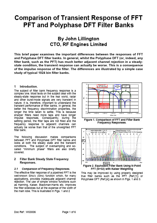
Comparison of Transient Response of FFT PFT and Polyphase DFT Filter BanksBy John LillingtonCTO, RF Engines LimitedThis brief paper examines the important differences between the responses of FFT and Polyphase DFT filter banks. In general, whilst the Polyphase DFT (or, indeed, any filter bank, such as the PFT) has much better adjacent channel rejection in a steady-state condition, the transient response can actually be worse. This is a consequence of the impulse response of the filter. The differences are illustrated by a simple case study of typical 1024 bin filter banks.1 Introduction.The subject of filter bank frequency response is a complex one. Most texts on the subject deal with the steady-state response but in the real world, radar and other burst-mode signals are very transient in nature. It is, therefore, important to understand the transient performance of filter banks. In general, the better the frequency discrimination properties, the longer the time taken to settle. This is because sharper filters need more taps and have longer impulse responses. Consequently, during the settling period, the filter taps are not filled and the frequency response to adjacent channels can actually be worse than that of the unweighted FFT filter bank.The following discussion makes comparisons between FFT and Polyphase DFT filter banks and looks at both the steady state and the transient conditions. The subject of oversampling and so-called “minimum phase” filters are also briefly covered.2 Filter Bank Steady State FrequencyResponses.2.1 Comparison of Frequency Responses.The effective filter response of a pipelined FFT is the well-known Sinx/x (Sinc) function which, for many applications, provides inadequate adjacent channel rejection. The use of simple window functions such as Hanning, Kaiser, Blackman-Harris etc. improves the filter sidelobes but at the expense of the width of the main lobe. This is illustrated in Figs. 1 and 2Figure 1. Comparison of FFT and Filter BankFrequency Responses.Input Bandwidth < +Channel Spacing = F-Fs/2+Fs/2FrequencyF s/ 2Input S/R = Fs (Complex)s/NPer-Channel Output S/R = F s/N (Complex)FFT (N=32) with Kaiser WeightingThis may be improved by using properly designed true filter banks such as the PFT (Ref.[1]) or Polyphase DFT (Ref.[4]) as shown in Figs. 1 and 3.0-Fs/2+Fs/2Frequency Channel Spacing = F s /NPer-Channel Output S/R = F s /N (Complex)Superior Cut-Off &Stop-Band Performance 2.2 Effective Noise Bandwidth. Another useful measure of filter performance is that of Effective Noise Bandwidth (ENB). Table 1 below gives a comparison between various filter banks. Table 1 Window Type ENB ENB(dB)Uniform 1.0 0.00Hanning 1.503 1.77Kaiser 1.656 2.19Blackman-Harris 2.006 3.023 Tap Poly, 0.1 dB Ripple, 100dB Stopband1.7562.44 4 Tap Poly, 0.1 dB Ripple, 100dB Stopband1.527 1.84 5 Tap Poly, 0.1 dB Ripple, 100dB Stopband 1.452 1.628 Tap Poly, 0.1 dB Ripple, 100dB Stopband1.276 1.06This shows, for example, that a Blackman-Harrisweighted FFT, whilst giving good sidelobes, will lose over 3 dB in signal-to-noise (S/N) whereas an 8 tap Polyphase DFT (i.e. a window 8x the transform length, as explained below) gives good sidelobes and low ENB, losing only 1 dB S/N. 3 General Time Domain Considerations.3.1 Windowing of Time Domain Samples.For simple windowing, the number of samples in the window will equal that of the transform itself. To achieve better filters requires the number of samples in the window to exceed that of the transform. This window can, in theory, be of any length. In the Polyphase DFT case, it is normally an integer number (2x, 3x etc.) times the transform length but in the WOLA implementation (Ref.[5]) it can be any length. Thus, for example, a 1024 bin filter bank might require 4096 input samples (4x frame length) for the first full output frame. For the PFT filter bank (Ref.[1]), the number of samples required is equivalent to the impulse response of the cascaded filters but the net effect is similar in that the number of samples required to achieve the first full frame of output data far exceeds the frame length.3.2 Oversampling.Another factor affecting the required processing throughput rate is the degree of oversampling required at the output filters. Even to achieve critical sampling (i.e. sample rate just equal to Nyquist)requires overlapped processing. Using the above example, 4096 samples are needed to form the first full output frame of 1024 bins. To achieve critical sampling means that the next frame of 1024 bins must be contiguous in time with the previous frameand that the output sample rate must be equal to theinput sample rate. This can be achieved only if thestart of the next set of 4096 samples is delayed by 1024 samples which requires 4 overlapped processes. To achieve over-sampling, increased overlap is required. Using the above example again,2x oversampling would require the 4096 samples tobe delayed by only 512 samples which requires 8 overlapped processes. A factor of 2x oversampling is standard in the PFT and higher factors can easily be achieved by simply not decimating in some of the stages, as shown in Fig. 4 below.Stages 1 or 2)For the Polyphase DFT, there are two elegant architectures that can be used. The WOLA structure is shown in Fig. 5 below.In this illustration, the window is around 4x the transform length, the windowed samples being sliced into 4 sections, overlapped in time and added before applying the FFT.The degree of oversampling is determined simply by the number of new samples, M, introduced for each new transform. The lower the value of M, the higher the oversampling factor.For integer oversampling, the polyphase structure of Fig. 6 below may be used. The input sample stream is decimated into K phases, filtered by an N-tap filter (K=1024 and N=4 in the above example) before applying the K-point DFT. Oversampling is achieved by up-sampling (zero stuffing) by a factor I. Thus, for 2x oversampling, I=2 etc. Note that this architecture can only be used with integer oversampling and gives exactly the same results as the WOLA structure with integer oversampling.Figure 6. Polyphase DFT Filter BankImplementation.4 Transient Analysis.4.1 General Parameters.Although the Polyphase, WOLA or PFT filter banks give much better adjacent channel rejection in the steady-state condition (i.e. for a steady signal condition and all filter taps filled), the transient response is quite another matter. Some early work on this subject is covered in Ref.[2] and is recommended reading. In the following discussion, the general parameters used are:-• No. of Bins = 1024• Input Sample Rate = 102.4 Ms/s (complex) • Output Sample Rate = 204.8 Ms/s (2x oversampled)• No. of Polyphase Taps = 5 (Equiv. To 5120 point window)• Filter Stopband = -85 dB• Filter Passband Ripple = 0.2 dB (pk-pk) • Filter Overlap = 75%The last parameter is a measure of the filter cut-off rate. The filters are designed to be flat to the edge of the bin and then reach the stopband level by 75% of the width of the adjacent bin.The transient results from a step function input of a sinewave input at a frequency offset from the centre by one half bin. This presents the worst spectral leakage case for the FFT.The graphs presented below are for normalised power spectra (10*Log10{I 2+Q 2}) and represent the pipelined output at the 2x oversampled rate (204.8 Ms/s in this case). An individual frame of 1024 samples contains the interleaved frequency bins from –Fs/2 to +Fs/2, where Fs is the input complex sample rate.4.2 FFT Transient Response.Fig. 7 below gives the response for an unweighted FFT. This does not show the “dead” time caused by the need to collect 1024 samples before the first output can be processed nor any other latency due to the actual hardware processing. Because it is 2x oversampled, the first 1024 point frame has not reached steady state. This can be explained by the fact that the first frame is produced in 5uS (1024 points at 204.8 Ms/s sample rate) whereas the inputFigure 7. Twice Oversampled, Unweighted, 1024Bin Pipelined FFT Transient Response. sample rate of 102.4 Ms/s means that only 512 samples are available (the remainder being zeros).The first frame is shown in more detail in Fig. 8 below.Figure 8. Frame 1 from Pipelined FFTFigure 9. Frame 2 from Pipelined FFTFig.9 shows the second frame which has now reached the steady state condition. This exhibits the expected Sinx/x sidelobe response for a signal which is one half-bin offset in frequency. This can be improved, as discussed above, by windowing the input data but at the expense of broadening the central lobe.4.3 Polyphase DFT Transient Response.Fig. 10 below gives the response for the 5 tap Polyphase DFT.Polyphase DFT Transient Response. Clearly the transient response is long compared with the FFT and has not fully settled to steady state until frame 10. Figs. 11, 12 and 13 show frames 1, 5 and10 respectively.Figure 11. 2x Oversampled Polyphase DFTFrame 1Figure 12. 2x Oversampled Polyphase DFTFrame 5Figure 13. 2x Oversampled Polyphase DFTFrame 10Even by frame 5, the effective filter frequency response is no better than an unweighted FFT. This is because the filter taps are still only half-full. It takes 10 frames (5 taps x oversampling factor) to reach the full steady state.4.4 Effect of Oversampling.It might be thought that the transients can be reduced through oversampling the output of the filter bank but this is not true . The transients are a function of the filter impulse response and the only effect of oversampling is to allow the transient to be seen in more detail. This may be illustrated by the following example:-• No. of Bins = 1024•Input Sample Rate = 6.4 Ms/s (complex)• Output Sample Rate = 204.8 Ms/s (32xoversampled)• No. of Polyphase Taps = 5 (Same effective filter as used above)Fig. 14 below gives the transient response for this32 times oversampled case. To keep the output sample rate at 204.8 Ms/s (limited by the maximum device output rate), the input rate must be reducedto 6.4 Ms/sPolyphase DFT Transient Response. Figures 16 and 17 below show the responses at frames 80 and 160 for the 32x oversampled case which correspond exactly to those of frames 5 and 10 for the 2x-oversampled case (Figs.12 & 13). This demonstrates clearly that there is no time advantage to be gained by oversampling. Frame 1 for the 32x case (Fig.15) is even less well developed than Frame 1 for the 2x case (Fig. 11) since there are now only 32 of the 5120 samples available. All this provides is more detail on the transient response as may be clearly seen by comparing Figs. 10 and 14 (note the different time axis scales due to the change of input sample rate from 102.4 Ms/s to 6.4Ms/s).Figure 15. 32x Oversampled Polyphase DFTFrame 1Figure 16. 32x Oversampled Polyphase DFTFrame 80Figure 17. 32x Oversampled Polyphase DFTFrame 160Allowing for the lower input sample rate, it may be seen that the only effect of oversampling is to observe greater detail in the transient response.4.5 Effect of Minimum Phase FIR Filters.This is discussed in some detail in Ref.[2]. A more accurate name would be “minimum group delay filters” since, in a similar manner to IIR filters, the group delay at centre-band may be reduced at the expense of a non-linear phase response. A typical example is shown in Fig. 18 below.Figure 18. 2x Oversampled 5 Tap, MinimumPhase, 1024 Bin, Polyphase DFT TransientResponse.The parameters are the same for those of Fig. 10 except that the filter tap coefficients are different. It may be seen that the amplitude response of the filter has a much faster “attack”. This does not necessarily mean that the filter actually settles fasterin the sense of adjacent channel rejection. This is best seen in Figs. 19, 20 and 21 below.Figure 19. Min. Phase Frame 1Figure 20. Min. Phase Frame 5Figure 21. Min. Phase Frame 10What this illustrates is that, by Frame 5, even though the amplitude has reached full level, the spectral response has still not reached the steady state condition of Frame 9 or 10. This effect is similar to that of the standard Polyphase DFT (see Fig. 12). 5 Conclusions.The conclusions are quite clear. Fast transient response and sharp spectral filters are not simultaneously achievable. The quickest settling is achieved by the plain old FFT (weighted or unweighted) at the expense of relatively poor spectral filtering. Another way of looking at this is to realise that the step response of the Sinx/x FFT filters is as near to an instant step as is achievable. Once we introduce ‘brick wall’ filters we must accept the consequent transient response delays caused by the filters needing to fill up. The sharper the filters, the longer the transients. If amplitude of the signal in a given bin is the main priority, then ‘minimum phase’ filters can help but this will not improve (and may actually worsen) the adjacent channel rejection during the transient period. It will also introduce a non linear phase response across each of the bins. Over-sampling may be useful in revealing more detail in the transient period but it will not shorten it.6 References.[1] PFT Architecture and Comparisons with FFT / DigitalDown-Converter Techniques./download/W02001-PFT WhitePaper.pdf[2] Comparison of the Transient Response of Different FilterBank Types./download/W02002-Transient Response White Paper.pdf[3] Pipelined FFT . /download/W02004-Pipelined FFT White Paper.pdf[4] D02003-Polyphase DFT Datasheet./download/D02003-Polyphase DFTdata sheet.pdf[5] Gumas, CC, “Window-presum FFT achieves high-dynamicrange, resolution”, Personal Engineering & InstrumentationNews, July 1997, pgs 58-64./dsp/DSP000315F1.html。

(I已打印)Non-singular terminal sliding mode control of rigid manipulators

Automatica38(2002)2159–2167/locate/automaticaBrief PaperNon-singular terminal sliding mode control of rigid manipulatorsYong Feng a,Xinghuo Yu b;∗,Zhihong Man ca Department of Electrical Engineering,Harbin Institute of Technology,Harbin150006,People’s Republic of Chinab School of Electrical and Computer Engineering,Royal Melbourne Institute of Technology University,GPO Box2476V Melbourne,Vic.3001,Australiac School of Computer Engineering,Nanyang Technological University,SingaporeReceived26June2001;received in revised form16June2002;accepted9July2002AbstractThis paper presents a global non-singular terminal sliding mode controller for rigid manipulators.A new terminal sliding mode manifold isÿrst proposed for the second-order system to enable the elimination of the singularity problem associated with conventional terminal sliding mode control.The time taken to reach the equilibrium point from any initial state is guaranteed to beÿnite time.The proposed terminal sliding mode controller is then applied to the control of n-link rigid manipulators.Simulation results are presented to validate the analysis.?2002Elsevier Science Ltd.All rights reserved.Keywords:Terminal sliding mode control;Singularity;Robotic manipulator;Robust control;Lyapunov stability1.IntroductionVariable structure systems(VSS)are well known for their robustness to system parameter variations and external disturbances(Slotine&Li,1991;Utkin,1992; Yurl&James,1988).VSS have been widely used in many applications,such as robots,aircrafts,DC and AC motors, power systems,process control and so on.An aspect of VSS that is of particular interest is the sliding mode control,which is designed to drive and constrain the system states to lie within a neighborhood of the pre-scribed switching manifolds that exhibit desired dynam-ics.When in the sliding mode,the closed-loopresp onse becomes totally insensitive to both internal parameter un-certainties and external disturbances.A characteristic of conventional VSS is that the convergence of the system states to the equilibrium point is usually asymptotical due to the asymptotical convergence of the linear switching manifolds that are commonly chosen.Recently,a terminal sliding mode(TSM)controller was developed(Man&Yu,1997;Yu&Man,1996;Wu,Yu,& This paper was not presented at any IFAC meeting.This paper was recommended for publication in revised form by Associate Editor Jurek Z.Sasiadek under the direction of Editor Mituhiko Araki.∗Corresponding author.E-mail addresses:yfeng@(Y.Feng),x.yu@.au(X.Yu).Man,1998).TSM has been used in the control of rigid ma-nipulators(Man et al.,1994;Tang,1998).The TSM con-cept is related to theÿnite time control(Haimo,1986; Bhat&Bernstein,1997).Compared with linear hyperplane-based sliding modes,TSM o ers some superior properties such as fast,ÿnite time convergence.This controller is par-ticularly useful for high precision control as it speeds up the rate of convergence near an equilibrium point.However,the existing TSM controller design methods still have a singu-larity problem.An initial discussion to avoid the singularity in TSM control systems was presented(Wu et al.,1998). In this paper,a global non-singular terminal sliding mode (NTSM)controller is presented for a class of nonlinear dy-namical systems with parameter uncertainties and external disturbances.A new NTSM manifold is proposed to over-come the singularity problem.The time taken to reach the manifold from any initial state and the time taken to reach the equilibrium point in the sliding mode can be guaran-teed to beÿnite time.The proposed NTSM controller is then applied to the control of n-degree-of-freedom rigid ma-nipulators.Simulation results are presented to validate the analysis.2.Conventional terminal sliding mode controlThe basic principle of TSM control can be brie y sum-marized as follows:consider a second-order uncertain0005-1098/02/$-see front matter?2002Elsevier Science Ltd.All rights reserved. PII:S0005-1098(02)00147-42160Y.Feng et al./Automatica 38(2002)2159–2167nonlinear dynamical system ˙x 1=x 2;˙x 2=f (x )+g (x )+b (x )u;(1)where x =[x 1;x 2]T is the system state vector,f (x )and b (x )=0are smooth nonlinear functions of x ,and g (x )represents the uncertainties and disturbances satisfying g (x ) 6l g where l g ¿0,and u is the scalar control in-put.The conventional TSM is described by the following ÿrst-order terminal sliding variables =x 2+ÿx q=p1;(2)where ÿ0is a design constant,and p and q are positive odd integers,which satisfy the following condition:p ¿q:(3)The su cient condition for the existence of TSM is 12d d ts 2¡−Á|s |;(4)where Á¿0is a constant.For system (1),a commonly used control design isu =−b −1(x ) f (x )+ÿq px q=p −11x 2+(l g +Á)sgn(s );(5)which ensures that TSM occurs.It is clear that if s (0)=0,the system states will reach the sliding mode s =0within the ÿnite time t r ,which satisÿes t r 6|s (0)|Á:(6)When the sliding mode s =0is reached,the system dy-namics is determined by the following nonlinear di erential equation:x 2+ÿx q=p 1=˙x 1+ÿx q=p1=0;(7)where x 1=0is the terminal attractor of the system (7).The ÿnite time t s that is taken to travel from x 1(t r )=0to x 1(t s +t r )=0is given byt s =−ÿ−1x 1(t r )d x 1x q=p 1=p ÿ(p −q )|x 1(t r )|1−q=p :(8)This means that,in the TSM manifold (7),both the system states x 1and x 2converge to zero in ÿnite time.It can be seen in the TSM control (5)that the secondterm containing x q=p −11x 2may cause a singularity to occur if x 2=0when x 1=0.This situation does not occur inthe ideal sliding mode because when s =0;x 2=−ÿx q=p1hence as long as q ¡p ¡2q ,i.e.1¡p=q ¡2,the term x q=p −11x 2is equivalent to x (2q −p )=p 1which is non-singular.The singularity problem may occur in the reaching phase when there is insu cient control to ensure that x 2=0while x 1=0.The TSM controller (5)cannot guarantee a bounded controlsignal for the case of x 2=0when x 1=0before the system states reach the TSM s =0.Furthermore,the singularity may also occur even after the sliding mode s =0is reached since,due to computation errors and uncertain factors,the system states cannot be guaranteed to always remain in the sliding mode especially near the equilibrium point (x 1=0;x 2=0),and the case of x 2=0while x 1=0may occur from time to time.This underlines the importance of addressing the singularity problem in conventional TSM systems.3.Non-singular terminal sliding mode controlIn order to overcome the singularity problem in the con-ventional TSM systems,several methods have been pro-posed.For example,one approach is to switch the sliding mode between TSM and linear hyperplane based sliding mode (Man &Yu,1997).Another approach is to transfer the trajectory to a pre-speciÿed open region where TSM control is not singular (Wu et al.,1998).These methods are adopting indirect approaches to avoid the singularity.In this paper,a simple NTSM is proposed,which is able to avoid this problem completely.The proposed NTSM model is de-scribed as follows:s =x 1+1ÿx p=q 2;(9)where ÿ;p and q have been deÿned in (2).One can easilysee that when s =0,the NTSM (9)is equivalent to (2)so that the time taken to reach the equilibrium point x 1=0when in the sliding mode is the same as in (8).Note that in using (9)the derivative of s along the system dynamics does not result in terms with negative (fractional)powers.This can be seen in the following theorem about the NTSM control.Theorem 1.For system (1)with the NTSM (9),if the control is designed asu =−b −1(x ) f (x )+ÿq px 2−p=q2+(l g +Á)sgn(s );(10)where 1¡p=q ¡2;Á¿0,then the NTSM manifold (9)will be reached in ÿnite time.Furthermore ,the states x 1and x 2will converge to zero in ÿnite time .Proof.For the NTSM (9),its derivative along the system dynamics (1)is ˙s =˙x 1+1ÿp q x p=q −12˙x 2=x 2+1ÿp q x p=q −12˙x 2=x 2+1ÿp q x p=q −12(f (x )+g (x )+b (x )u )Y.Feng et al./Automatica38(2002)2159–21672161=x2+1ÿpqx p=q−12g(x)−ÿqpx2−p=q2−(l g+Á)sgn(s)=1ÿpqx p=q−12(g(x)−(l g+Á)sgn(s))thens˙s=1ÿpqx p=q−12(g(x)s−(l g+Á)sgn(s)s)6−1ÿpqÁx p=q−12|s|:Since p and q are positive odd integers and1¡p=q¡2,there is x p=q−12¿0for x2=0.Let (x2)=(1=ÿ)(p=q)Áx p=q−12.Then it hass˙s6− (x2)|s|(x2)¿0for x2=0:(11)Therefore,for the case x2=0,the condition for Lya-punov stability is satisÿed.The system states can reach the sliding mode s=0withinÿnite ing the following ar-guments can easily prove this:substituting the control(10) into system(1)yields˙x2=−ÿqpx2−p=q2+g(x)−(l g+Á)sgn(s):Then,for x2=0,it is obtained˙x2=g(x)−(l g+Á)sgn(s):For both s¿0and s¡0,it is obtained˙x26−Áand ˙x2¿Á,respectively,showing that x2=0is not an attractor.It also means that there exists a vicinity of x2=0such that for a small ¿0such that|x2|¡ ,there are˙x26−Áfor s¿0 and˙x2¿Áfor s¡0,respectively.Therefore,the crossing of the trajectory from the boundary of the vicinity x2= to x2=− for s¿0,and from x2=− to x2= for s¡0occurs inÿnite time.For other regions where|x2|¿ ,it can be easily concluded from(11)that the switching line s=0can be reached inÿnite time since we have˙x26−Áfor s¿0 and˙x2¿Áfor s¡0.The phase plane plot of the system is shown in Fig.1.Therefore,it is concluded that the sliding mode s=0can be reached from anywhere in the phase plane inÿnite time.Once the switching line is reached,one can easily see that NTSM(9)is equivalent to the TSM(2),so the time taken to reach the equilibrium point x1=0in the sliding mode is the same as in(8).Therefore,the NTSM manifold(9)can be reached inÿnite time.The states in the sliding mode will reach zero inÿnite time.This completes the proof.Remark1.It should be noted that the NTSM control(10) is always non-singular in the state space since1¡p=q¡2.Remark2.In order to eliminate chattering,a saturation function sat can be used to replace the sign function sgn.The1Fig.1.The phase plot of the system.relationshipbetween the steady-state errors of the NTSM system and the width of the layer surrounding the NTSM manifold s(t)=0is given by(Feng,Han,Stonier,&Man, 2000;Feng,Yu,&Man,2001)|s(t)|6’⇒|x(t)|6’and|x(t)|6(2ÿ’)q=p for t→∞:(12)4.Non-singular terminal sliding mode control for rigid manipulatorsIn this section,a non-singular terminal sliding mode con-trol is designed for the rigid n-link robot manipulatorM(q) q+C(q;˙q)+g(q)= (t)+d(t);(13) where q(t)is the n×1vector of joint angular position,M(q) the n×n symmetric positive deÿnite inertia matrix,C(q;˙q) the n×1vector containing Coriolis and centrifugal forces, g(q)the n×1gravitational torque,and (t)n×1vector of applied joint torques that are actually the control inputs,and d(t)n×1bounded input disturbances vector.It is assumed that rigid robotic manipulators have uncertainties,i.e.:M(q)=M0(q)+ M(q);C(q;˙q)=C0(q;˙q)+ C(q;˙q);g(q)=g0(q)+ g(q);where M0(q);C0(q;˙q)and g0(q)are the estimated terms; M(q); C(q;˙q)and g(q)are uncertain terms.Then, the dynamic equation of the manipulator can be written in the following form:M0(q) q+C0(q;˙q)+g0(q)= (t)+ (t)(14)2162Y.Feng et al./Automatica 38(2002)2159–2167with(t )=− M (q ) q − C (q ;˙q )q − g (q ):(15)The following assumptions are made about the robot dy-namics: M (q ) ¡ 0;(16) C (q ;˙q ) ¡ÿ0+ÿ1 q +ÿ2 ˙q 2;(17) g (q ) ¡ 0+ 1 q ;(18) (t ) ¡ 0+ 1 q + 2 ˙q 2;(19) (t ) ¡b 0+b 1 q +b 2 ˙q 2;(20)where 0;ÿ0;ÿ1;ÿ2; 0; 1; 0; 1; 2;b 0;b 1;b 2are positivenumbers.Suppose that q r is the desired input of the robot mani-pulator and ˙q r is the derivative of q r .Deÿne ”(t )=q −q r ;˙”(t )=˙q −˙q r ;e (t )=[”T (t )˙”T (t )]T .Then,the error equation of the rigid robotic manipulator can be obtained as follows:˙e (t )=Ae +B ;(21)whereA = 0I 00 ;B =0I;=M −10(q )(−C 0(q ;˙q )−g 0(q )−M 0(q ) q r + (t )+ (t )):It can be observed that the error dynamics (21)is of form (13).The NTSM control strategy developed in Section 3can be applied.The result is summarized in the following theorem.Before proceeding further,the notation of the frac-tional power of vectors is introduced.For a variable vector z ∈R n ,the fractional power of vectors is deÿned asz q=p =(z q=p 1;z q=p 2;:::;z q=p n )T;˙z q=p =(˙z q=p 1;˙z q=p 2;:::;˙zq=p n )T:Theorem 2.For the rigid n -link manipulator (14),if the NTSM manifold is chosen as s =”+C 1˙”p=q ;(22)where C 1=diag [c 11;:::;c 1n ]is a design matrix ,and the NTSM control is designed as follows ,then the system tracking error ”(t )will converge to zero in ÿnite time . = 0+u 0+u 1;(23)where0=C 0(q ;˙q )+g 0(q )+M 0(q ) q r ;(24)u 0=−q pM 0(q )C −11˙”2−p=q;(25)u 1=−q p [s T C 1diag (˙”p=q −1)M −10(q )]T s T C 1diag (˙”p=q −1)M −10(q )×[ s C 1diag (˙”p=q −1)M −10(q ) (b 0+b 1 q+b 2 ˙q 2)];(26)where b 0;b 1;b 2are supposed to be known parameters as in (20).Proof.Consider the following Lyapunov functionV =12s Ts :Di erentiating V with respect to time,and substituting (23)–(26)into it yields˙V =s T ˙s =s T ˙”+p qC 1diag (˙”p=q −1) ”=s T ˙”+p q C 1diag (˙”p=q −1)M −10(q )(u 1(t )+u 0(t ))+ (t ))=s T p q C 1diag (˙”p=q −1)M −10(q )(u 1(t )+ (t )) =−p qs C 1diag (˙”p=q −1)M −10(q ) ×(b 0+b 1 q +b 2 ˙q 2)+p qs T C 1diag (˙”p=q −1)M −10(q ) (t )6−p qs C 1diag (˙”p=q −1)M −10(q ) ×(b 0+b 1 q +b 2 ˙q 2)+p qs C 1diag (˙”p=q −1)M −10(q ) (t ) =−p qC 1diag (˙”p=q −1)M −10(q ) ×(b 0+b 1 q +b 2 ˙q 2− (t ) ) s that is˙V 6−Á(t ) s ¡0for s =0;(27)where Á(t )=p qC 1diag (˙”p=q −1)M −10(q ) ×{(b 0+b 1 q +b 2 q 2)− (t ) }¿0:Therefore,according to the Lyapunov stability criterion,the NTSM manifold s (t )in (22)converges to zero in ÿ-nite time.On the other hand,if s =”+C 1˙”p=q =0are reached as shown in Theorem 1,then the output trackingY.Feng et al./Automatica38(2002)2159–21672163 error of the robot manipulator”(t)=q−q r will convergeto zero inÿnite time.This completes the proof.Remark3.The NTSM control proposed in Theorem2solves the control of the rigid n-link manipulator,that repre-sents a special class of problems.The method proposed canbe extended to a class of n-order(n¿2)nonlinear dynam-ical systems,that represents a broader class of problems:˙x1=f1(x1;x2);˙x2=f2(x1;x2)+g(x1;x2)+B(x1;x2)u;(28)where x1=(x11;x12;:::;x1n)T∈R n;x2=(x21;x22;:::;x2n)T∈R n;f1and f2are smooth vector functions and g rep-resents the uncertainties and disturbances satisfyingg(x1;x2) 6l g where l g¿0;B is a non-singular ma-trix and u=(u1;u2;:::;u n)T∈R n is the control vector.It is further assumed that(x1;x2)=(0;0)if and only if(x1;˙x1)=(0;0).Note that many practical dynamical sys-tems satisfy this condition,for example,the mechanicalsystems.Robotic systems are certainly a special case of(28).Actually,the robotic system(14)is not in the form of(28),but it can be transformed to such form by the coordi-nates change.So,the proposed algorithm in the paper can beapplied to any plant,which can be transformed to(28).TheNTSM for system(28)can be designed as follows.Chooses=x1+ ˙x p=q1;(29)where =diag( 1;:::; n);( i¿0)for i=1;:::;n,and˙x p=q1is represented as˙x p=q1=(x p1=q111;:::;x p n=q n1n)T:If the NTSM control is designed as in(30),then the high-order nonlinear dynamical systems(28)will converge to the NTSM and the equilibrium point inÿnite time,re-spectively,u=−@f1@x2B(x1;x2)−1l g@f1@x2+Áss+@f1@x1f1(x1;x2)+@f1@x2f2(x1;x2)+ −1 −1diag(x2−p1=q q11;:::;x2−p n=q n1n);(30)where =diag(p1=q1;:::;p n=q n);p i and q i are positive odd integers and q i¡p i¡2q i for i=1;:::;n.5.Simulation studiesThe section presents two studies:one is the comparison study of performance between NTSM and TSM,and the other an application to a robot control problem.-0.0500.050.10.150.20.250.3-0.4-0.20.20.40.60.81.0x1x2Fig.2.Phase plot of NTSM system.parison studyIn order to analyze the e ectiveness of the NTSM control proposed and to compare NTSM with TSM,consider the simple second-order dynamical system below:˙x1=x2;˙x2=0:1sin20t+u:(31) The NTSM and TSM are chosen as follows:s NTSM=x1+x5=32;s TSM=x2+x3=51:Three control approaches are adopted:NTSM control, TSM control,and indirect NTSM control.The NTSM con-trol is designed according to(10)and NTSM(9),and TSM control is designed according to(5)and TSM(2).The in-direct NTSM control is designed in the same way as TSM, with only one di erence,that is when|x1|¡ ,let p=q, and is selected as0.001(Man&Yu,1997).Three sys-tems achieve the same terminal sliding mode behavior.So, only the phase plane response of the NTSM control system is provided,as shown in Fig.2.The control signals for the three kinds of systems are shown in Figs.3–5.It can be ob-viously seen some valuable facts.No singularity occurs at all in the case of NTSM control.When the trajectory crosses the x1=0axis,singularity occurs in the case of TSM con-trol.For the indirect NTSM control,although singularity is avoided by switching from the TSM to linear sliding mode, the e ect of the singularity can be seen,especially when decreases to zero.However when is relatively large, the sliding mode of the system is switching between TSM and the linear plane based sliding mode,and the advantage of TSM system is lost.Therefore,from the results of the above simulations,the occurrence of singularity problem in the TSM system,the drawback of the indirect NTSM,and the e ectiveness of the NTSM in avoiding singularity,are observed,respectively.2164Y.Feng et al./Automatica 38(2002)2159–21670.51.0 1.52.02.5-8-7-6-5-4-3-2-1012time (sec.)uFig.3.Control signal of NTSM system.0.51.0 1.52.02.5-90-80-70-60-50-40-30-20-10010time(sec.)uFig.4.Control signal of TSM system.5.2.Control of a robotA simulation with a two-link rigid robot manipulator (seeFig.6)is performed for the purpose of evaluating the perfor-mance of the proposed NTSM control scheme.The dynamic equation of the manipulator model in Fig.6is given by a 11(q 2)a 12(q 2)a 12(q 2)a 22q 1 q 2 +−ÿ12(q 2)˙q 21−2ÿ12(q 2)˙q 1˙q 2ÿ12(q 2)˙q 22+ 1(q 1;q 2)g 2(q 1;q 2)g =1 2;(32)0.51.0 1.52.02.5-8-7-6-5-4-3-2-1012time(sec.)uFig.5.Control signal of indirect TSMsystem.Fig.6.Two-link robot manipulator model.wherea 11(q 2)=(m 1+m 2)r 21+m 2r 22+2m 2r 1r 2cos(q 2)+J 1;a 12(q 2)=m 2r 22+m 2r 1r 2cos(q 2);a 22=m 2r 22+J 2;ÿ12(q 2)=m 2r 1r 2sin(q 2);1(q 1;q 2)=((m 1+m 2)r 1cos(q 2)+m 2r 2cos(q 1+q 2)); 2(q 1;q 2)=m 2r 2cos(q 1+q 2):The parameter values are r 1=1m ;r 2=0:8m ;J 1=5kg m ;J 2=5kg m ;m 1=0:5kg ;m 2=1:5kg.The desired reference signals are given by q r 1=1:25−(7=5)e −t +(7=20)e −4t ;q r 2=1:25+e −t −(1=4)e −4t :The initial values of the system are selected as q 1(0)=1:0;q 2(0)=1:5;˙q 1(0)=0:0;˙q 2(0)=0:0:Y.Feng et al./Automatica 38(2002)2159–216721650123456789100.20.40.60.81.01.21.41.6time(sec)O u t p u t t r a c k i n g o f j o i n t 1( r a d )Fig.7.Output tracking of joint 1using a boundary layer.123456789101.21.31.41.51.61.71.81.92.0time(sec)O u t p u t t r a c k i n g o f j o i n t 2( r a d )Fig.8.Output tracking of joint 2using a boundary layer.The nominal values of m 1and m 2are assumed to be ˆm 1=0:4kg ;ˆm 2=1:2kg :The boundary parameters of system uncertainties in (20)are assumed to be b 0=9:5;b 1=2:2;b 2=2:8:Suppose the tracking error and the 1st tracking error are tobe |˜q i |60:001and |˙˜q i |60:024;i =1,2,where ˜q i =q i −q riand ˙˜q i =˙q i −˙q ri ;i =1,ing the above performance index,it can be determined the parameters of NTSM manifolds.According to (12),it is obtained that |˜q i |6’i ;i =1;2:Let ’i =0:001;i =1;2(33)012345678910-15-10-5051015202530time(sec)C o n t r o l i n p u t o f j o i n t 1( N m )Fig.9.Control of joint 1using a boundary layer.12345678910-14-12-10-8-6-4024time(sec)C o n t r o l i n p u t o f j o i n t 2 (N m )Fig.10.Control of joint 2using a boundary layer.the tracking error of the system |˜q i |can be guaranteed.Onthe other hand,according to (12),it is obtained that |˙˜q i |6(2ÿ’i )q=p ;i =1;2:Let(2ÿ’i )q=p 60:024;i =1;2;thenq p6log 0:024log(2ÿ’i );i =1;2:(34)For simplicity,let ÿi =1;i =1;2.Then from (34),it is obtained thatq p 6log 0:024log(2×1×0:001)=0:60015;i =1;2:(35)2166Y.Feng et al./Automatica 38(2002)2159–2167-0.100.10.20.30.40.50.60.70.80.9-0.9-0.8-0.7-0.6-0.5-0.4-0.3-0.2-0.100.1e1(t)(rad)d e 1/d t (r a d /s )Fig.11.Phase plot of tracking error of joint 1.-0.5-0.4-0.3-0.2-0.10.100.20.30.40.50.6e2(t)(rad)d e 2/d t (r a d /s )Fig.12.Phase plot of tracking error of joint 2.Let qp=0:6:Now,the parameters of the TSM can be obtained as:q =3;p =5(there are many other options as well).Finally,the NTSM models are obtained as follows:s 1=˜q 1+˙˜q 5=31=0;s 2=˜q 2+˙˜q 5=32=0:In order to eliminate the chattering,the boundary layermethod is adopted (Slotine &Li,1991)in the NTSM con-trol.The simulation results are shown in Figs.7–12.Figs.7and 8show the output tracking of joints 1and 2.Figs.9and 10depict the control signals of joints 1and 2,respec-tively.Figs.11and 12show the phase plot of tracking error of joints 1and 2,respectively.One can easily see that the system states track the desired reference signals.First,theoutput tracking errors of the system reach the terminal slid-ing mode manifold s =0in ÿnite time,then they converge to zero along s =0in ÿnite time.It can be clearly seen that neither singularity nor chattering occurs in the two control signals.6.ConclusionsIn this paper,a global non-singular TSM controller for a second-order nonlinear dynamic systems with parameter uncertainties and external disturbances has been proposed.The time taken to reach the manifold from any initial sys-tem states and the time taken to reach the equilibrium point in the sliding mode have been proved to be ÿnite.The new terminal sliding mode manifold proposed can enable the elimination of the singularity problem associated with con-ventional terminal sliding mode control.The global NSTM controller proposed has been used for the control design of an n -degree-of-freedom rigid manipulator.Simulation results are presented to validate the analysis.The proposed controller can be easily applied to practical control of robots as given the advances of microprocessors,the vari-ables with fractional power can be easily built into control algorithms.ReferencesBhat,S.P.,&Bernstein, D.S.(1997).Finite-time stability of homogeneous systems.Proceedings of American control conference (pp.2513–2514).Feng,Y.,Han,F.,Yu,X.,Stonier,D.,&Man,Z.(2000).Tracking precision analysis of terminal sliding mode control systems with saturation functions.In X.Yu,J.-X.Xu (Eds.),Advances in variable structure systems :Analysis,integration and applications (pp.325–334).Singapore:World Scientiÿc.Feng,Y.,Yu,X.,&Man,Z.(2001).Non singular terminal sliding mode control and its applications to robot manipulators.Proceedings of 2001IEEE international symposium on circuits and systems ,Vol.III (pp.545–548).Sydney,May 2001.Haimo,V.T.(1986).Finite time controllers.SIAM Journal of Control and Optimization ,24(4),760–770.Man,Z.,Paplinski,A.P.,&Wu,H.(1994).A robust MIMO terminal sliding mode control scheme for rigid robotic manipulators.IEEE Transactions on Automatic Control ,39(12),2464–2469.Man,Z.,&Yu,X.(1997).Terminal sliding mode control of mimo linear systems.IEEE Transactions on Circuits and Systems I:Fundamental Theory and Applications ,44(11),1065–1070.Slotine,J.E.,&Li,W.(1991).Applied non-linear control .Englewood Cli s,NJ:Prentice-Hall.Tang,Y.(1998).Terminal sliding mode control for rigid robots.Automatica ,34(1),51–56.Utkin,V.I.(1992).Sliding modes in control optimization .Berlin,Heidelberg:Springer.Wu,Y.,Yu,X.,&Man,Z.(1998).Terminal sliding mode control design for uncertain dynamic systems.Systems and Control Letters ,34,281–288.Yu,X.,&Man,Z.(1996).Model reference adaptive control systems with terminal sliding modes.International Journal of Control ,64(6),1165–1176.Yurl,B.S.,&James,M.B.(1988).Continuous sliding mode control.Proceedings of American Control Conference (pp.562–563).Y.Feng et al./Automatica 38(2002)2159–21672167Yong Feng received the B.S.degree from the Department of Control Engineering in 1982,and M.S.degree from the Depart-ment of Electrical Engineering in 1985and Ph.D.degree from the Department of Con-trol Engineering in 1991,in Harbin Insti-tute of Technology,China,respectively.He has been with the Department of Electri-cal Engineering,Harbin Institute of Tech-nology since 1985,and is currently a Pro-fessor.He was a visiting scholar in the Faculty of Informatics and Communication,Australia,from May 2000to November 2001.He has authored and co-authored over 50journal and conference papers.He has published 3books.He has completed over 10research projects,including process control,arc welding robot,climbing wall robot,CNC system,a direct drive motor and its control system,the electronics and simulation of CCD digital camera,and so on.His current research interests are nonlinear control systems,sampled data systems,robot control,digital camera modelling andsimulation.Xinghuo Yu received B.Sc.(EEE)and M.Sc.(EEE)from the University of Sci-ence and Technology of China in 1982and 1984respectively,and Ph.D.degree from South-East University,China in 1987.From 1987to 1989,he was Research Fellow with Institute of Automation,Chi-nese Academy of Sciences,Beijing,China.From 1989to 1991,he was a Postdoctoral Fellow with the Applied Mathematics De-partment,University of Adelaide,Australia.From 1991to 2002,he was with CentralQueensland University,Rockhampton,Australia where he was Lecturer,Senior Lecturer,Associate Professor then Professor of Intelligent Sys-tems and the Associate Dean (Research)of the Faculty of Informatics and Communication.Since March 2002,he has been with the School of Electrical and Computer Engineering at Royal Melbourne Institute of Technology,Australia,where he is a Professor,Director of Software and Networks,and Deputy Head of School.He has also held Visiting Profes-sor positions in City University of Hong Kong and Bogazici University(Turkey).He has recently been conferred as Honorary Professor of Cen-tral Queensland University.He is Guest Professor of Harbin Institute of Technology (China),Huazhong University of Science and Technology (China),and Southeast University (China).Professor Yu’s research inter-ests include sliding mode and nonlinear control,chaos and chaos control,soft computing and applications.He has published over 200refereed pa-pers in technical journals,books and conference proceedings.He has also coedited four research books “Complex Systems:Mechanism of Adapta-tion”(IOS Press,1994),“Advances in Variable Structure Systems:Anal-ysis,Integration and Applications”(World Scientiÿc,2001),“Variable Structure Systems:Towards the 21st Century”(Springer-Verlag,2002),“Transforming Regional Economies and Communities with Information Technology”(Greenwood,2002).Prof.Yu serves as an Associate Editor of IEEE Trans Circuits and Systems Part I and is on the Editorial Board of International Journal of Applied Mathematics and Computer Science.He was General Chair of the 6th IEEE International Workshopon Variable Structure Systems held in December 2000on the Gold Coast,Australia.He was the sole recipient of the 1995Central Queensland University Vice Chancellor’s Award forResearch.Zhihong Man received the B.E.degree from Shanghai Jiaotong University,China,the M.S.degree from the Chinese Academy of Sciences,and the Ph.D.from the Uni-versity of Melbourne,Australia,all in electrical and electronic engineering,in 1982,1986and 1993,respectively.From 1994to 1996,he was a Lecturer in the Department of Computer and Commu-nication Engineering,Edith Cowan Uni-versity,Australia.From 1996to 2000,he was a Lecturer and then a SeniorLecturer in the Department of Electrical Engineering,the University of Tasmania,Australia.In 2001,he was a Visiting Senior Fellow in the School of Computer Engineering,Nanyang Technological University,Singapore.Since 2002,he has been an Associate Professor of Computer Engineering at Nanyang Technological University.His research interests are in robotics,fuzzy logic control,neural networks,sliding mode control and adaptive signal processing.He has published more than 120journal and conference papers in these areas.。

信号完整性和电源完整性分析

An Integrated Signal and Power Integrity Analysis for Signal Traces Through the Parallel Planes Using Hybrid Finite-Element andFinite-Difference Time-Domain TechniquesWei-Da Guo,Guang-Hwa Shiue,Chien-Min Lin,Member,IEEE,and Ruey-Beei Wu,Senior Member,IEEEAbstract—This paper presents a numerical approach that com-bines theﬁnite-element time-domain(FETD)method and theﬁ-nite-difference time-domain(FDTD)method to model and ana-lyze the two-dimensional electromagnetic problem concerned in the simultaneous switching noise(SSN)induced by adjacent signal traces through the coupled-via parallel-plate structures.Applying FETD for the region having the source excitation inside and FDTD for the remaining regions preserves the advantages of both FETD ﬂexibility and FDTD efﬁciency.By further including the transmis-sion-line simulation,the signal integrity and power integrity is-sues can be resolved at the same time.Furthermore,the numer-ical results demonstrate which kind of signal allocation between the planes can achieve the best noise cancellation.Finally,a com-parison with the measurement data validates the proposed hybrid techniques.Index Terms—Differential signaling,ﬁnite-element andﬁnite-difference time-domain(FETD/FDTD)methods,power integrity (PI),signal integrity(SI),simultaneous switching noise(SSN), transient analysis.I.I NTRODUCTIONI N RECENT years,considerable attention has been devotedto time-domain numerical techniques to analyze the tran-sient responses of electromagnetic problems.Theﬁnite-differ-ence time-domain(FDTD)method proposed by Yee in1966 [1]has become the most well-known technique because it pro-vides a lot of attractive advantages:direct and explicit time-marching scheme,high numerical accuracy with a second-order discretization error,stability condition,easy programming,and minimum computational complexity[2].However,it is often in-efﬁcient and/or inaccurate to use only the FDTD method to dealManuscript received March3,2006;revised November6,2006.This work was supported in part by the National Science Council,Republic of China,under Grant NSC91-2213-E-002-109,by the Ministry of Education under Grant93B-40053,and by Taiwan Semiconductor Manufacturing Company under Grant 93-FS-B072.W.-D.Guo,G.-H.Shiue,and R.-B.Wu are with the Department of Electrical Engineering and Graduate Institute of Communication Engi-neering,National Taiwan University,10617Taipei,Taiwan,R.O.C.(e-mail: f92942062@.tw;d9*******@.tw;rbwu@.tw).C.-M.Lin is with the Packaging Core Competence Department,Advanced Assembly Division,Taiwan Semiconductor Manufacturing Company,Ltd., 30077Taiwan,R.O.C.(e-mail:chienmin_lin@).Color versions of one or more of theﬁgures in this paper are available online at .Digital Object Identiﬁer10.1109/TADVP.2007.901595with some speciﬁc structures.Hybrid techniques,which com-bine the desirable features of the FDTD and other numerical schemes,are therefore being developed to improve the simula-tion capability in solving many realistic problems.First,the FDTD(2,4)method with a second-order accuracy in time and a fourth-order accuracy in space was incorporated to tackle the subgridding scheme[3]and a modiﬁed form was employed to characterize the electrically large structures with extremely low-phase error[4].Second,the integration with the time-domain method of moments was performed to analyze the complex geometries comprising the arbitrary thin-wire and inhomogeneous dielectric structures[5],[6].Third,theﬂexible ﬁnite-element time-domain(FETD)method was introduced locally for the simulation of structures with curved surfaces [6]–[8].With the advent of high-speed digital era,the simultaneous switching noise(SSN)on the dc power bus in the multilayer printed circuit boards(PCBs)causes paramount concern in the signal integrity and power integrity(SI/PI)along with the electromagnetic interference(EMI).One potential excitation mechanism of this high-frequency noise is from the signal traces which change layers through the via transition[9]–[11]. In the past,the transmission-line theory and the two-dimen-sional(2-D)FDTD method were combined successfully to deal with the parallel-plate structures having single-ended via transition[12],[13].Recently,the differential signaling has become a common wiring approach for high-speed digital system designs in beneﬁt of the higher noise immunity and EMI reduction.Nevertheless,for the real layout constraints,the common-mode currents may be generated from various imbal-ances in the circuits,such as the driver-phase skew,termination diversity,signal-path asymmetries,etc.Both the differential-and common-mode currents can inﬂuence the dc power bus, resulting in the SSN propagating within the planes.While applying the traditional method to manage this case,it will need a muchﬁner FDTD mesh to accurately distinguish the close signals transitioning through the planes.Such action not only causes the unnecessary waste of computer memory but also takes more simulation time.In order to improve the computa-tional efﬁciency,this paper incorporates the FETD method to the small region with two or more signal transitions inside,while the other regions still remain with the coarser FDTD grids.While the telegrapher’s equations of coupled transmission lines are further introduced to the hybrid FETD/FDTD techniques,the1521-3323/$25.00©2007IEEEFig.1.A typical four-layer differential-via structure.SI/PI co-analysis for differential traces through the planes can be accomplished as demonstrated in Section II and the numerical results are shown in Section III.For a group of signal vias,the proposed techniques can also tell which kind of signal alloca-tion to achieve the best performance as presented in Section III. Section IV thus correlates the measurement results and their comparisons,followed by brief conclusions in Section V.II.S IMULATION M ETHODOLOGYA typical differential-via structure in a four-layer board is il-lustrated in Fig.1.Along the signal-ﬂow path,the whole struc-ture is divided into three parts:the coupled traces,the cou-pled-via discontinuities,and the parallel plates.This section will present how the hybrid techniques integrate the three parts to proceed with the SI/PI co-simulation.At last,the stability consideration and computational complexity of the hybrid tech-niques are discussed as well.A.Circuit SolverWith reference to Fig.2,if the even/odd mode propagation coefﬁcients and characteristic impedances are given,it is recog-nized that the coupled traces can be modeled by theequivalentladder circuits,and the lossy effects can be well approxi-mated with the average values ofindividualand overthe frequency range of interest.The transient signal propagationis thus characterized by the telegrapher’s equations with the cen-tral-difference discretization both in time and space domains.The approach to predict the signal propagation through the cou-pled-via discontinuities is similar to that through the coupledtraces except for the difference of model-extracting method.To characterize the coupled-via discontinuities as depicted inFig.1,the structure can be separated into three segments:the viabetween the two solid planes,and the via above(and under)theupper(and lower)plane.Since the time delay of signals througheach segment is much less than the rising edge of signal,the cou-pled-via structure can be transformed into a SPICE passive net-work sketched in Fig.3by full-wave simulation[14],whererepresents the voltage of SSN induced by thecurrent on Ls2.By linking the extracted circuit models of coupled-via disconti-nuities,both the top-and bottom-layer traces together with suit-able driving sources and load terminations,the transient wave-forms throughout the interconnects are then characterized andcan be used for the SIanalyses.Fig.2.The k th element of equivalent circuit model of coupled transmissionlines.Fig.3.Equivalent circuit model of coupled-via structures.B.Plane SolverAs for the parallel-plate structure,because the separationbetween two solid planes is much smaller than the equiva-lent wavelength of signals,the electromagneticﬁeld inside issupposed to be uniform along the vertical direction.Thence,the2-D numerical technique can be applied to characterizethe SSN effects while the FETD method is set for the smallregion covering the signal transitions and the FDTD scheme isconstructed in the most regular regions.The FETD algorithm[15]starts from Maxwell’s two curl-equations and the vector equation is obtainedbyin(1)whereand denote the electricﬁeld and current density,re-spectively,in the losslessvolume.Applying the weak-formformulation or the Galerkin’s procedure to(1)gives(2)where is the weighting function that can be arbitrarily de-ﬁned.In use of theﬁnite-element method,the variational for-mula is thus discretized to implement the later numerical com-putation.In the present case,the linear basis function is chosento express theﬁelds inside each triangular element.After takingthe volume integration over each element and assembling theFig.4.FEM mesh in the source region and its interface with the FDTD grids. integrals from all the elements,(2)can be simpliﬁed into a ma-trix formof(3)whereand are the coefﬁcient vectors of electricﬁeld andcurrent density,respectively.In addition,the values of all matrixelements in(3)are formulatedasand(4)For the mesh proﬁle as illustrated in Fig.4,the FETD re-gion is chosen to be a block replacing the prime FDTD regioninto which the via transition penetrates.This is an initial valueproblem in time with thepreviousand being theinitial conditions as well as the boundary value problem in spacewith being Dirichlet boundary condition.To solve theinitial value problem in(3),the time derivative of electricﬁeldis approximated by the central difference,thatis(5)As for the electricﬁeld in the second term of(3),it can be for-mulated by the Newmark–Beta scheme[16]to be readas(6)Fig.5.Simulationﬂowchart of hybrid FETD and FDTD techniques to performthe SI/PI co-analysis for the coupled-via structure as illustrated in Fig.1.Moreover,in the triangular elements with the via transitioninside,the term in(3)as expressedbygridarea(7)is needed to serve as the excitation of the parallel-plate structurewith thecurrent shown in Fig.3through the via structurebetween Layers2and3.It is worth noting that the via transitionshould be placed on the bary-center of each triangular elementto achieve better accuracy.The hand-over scheme for theﬁeld in the overlapped region ofFDTD and FETD can be depicted in Fig.5.Given the boundaryﬁeld calculated by the FDTD algorithm at the timestep,all theﬁeld in the FETD region can be acquiredthrough the matrix solution of(3).The SSNvoltage in Fig.3is then determinedby(8)where is the averaging value of nodal electric-ﬁeldsenclosing the via transition,and is the separation between theplanes.Onceand at the FETD mesh nodes(node1,2,3,and4in Fig.4)become available,together with the ob-tained voltage/current values from the circuit solver and electric/magneticﬁelds of the FDTD region,the hybrid time-marchingscheme for the next time step can be implemented and so on.As a result of using the integrated schemes,thecurrent,arisen from the input signal through the via structure,can havethe ability to induce the voltage noise propagating within theFig.6.Physical dimensions of coupled traces and via pair.(a)Top view (Unit =mil ).(b)Side view.parallel plates.After a period of time,owing to the plane reso-nance and return path,the induced noise will cause the unwanted voltage ﬂuctuation on the coupled traces by the presence of the ﬁnite SSNvoltage .C.Stability Problem and Computational Complexity It is not dif ﬁcult to manifest that the FETD algorithm is un-conditionally stable.Substituting (5),(6),and (7)into (3)yields the following differenceequation:(9)where(10)the superscript “1”denotes the matrix inverse and thefactorgridareaWithout loss of generality,the time-stepping scheme in (9)is restatedas(11)Applyingthe -transform technique to (11)and solvingfor,de ﬁned asthe -transformof ,the resultreads(12)along with thedependent ,de ﬁned asthe -transformof in (11).Regardless of the timestep ,it can be easily de-duced that the poles of (12)is just on the unit circleof plane.This proves that the time marching by (9)is absolutely stable.The stability condition of these hybrid techniques is thus gov-erned by the transmission-line theory and the FDTD algorithm in the regular region,which are already known.Concerning the computational complexity,because of the consistence of simulation engines used for the circuitsolver,parison of differential-mode S -parameters from HFSS simulation and the equivalent circuit as depicted in Fig.3.the only work is to compare the ef ﬁciency of the hybrid FETD/FDTD technique with that of the traditional FDTD method.In use of only the FDTD scheme for cell discretization,the grid size should be chosen at most the spacing between the adjacent via transitions.However,as depicted in Fig.4,the hybrid techniques adopting the FEM mesh for the source region exhibit the great talent to segment the whole plane with the coarser FDTD grids.Owing to the sparsity of the FETD matrices in (4)and the much smaller number of unknowns,the computational time needed for each FETD operation can be negligible.The complexity of the hybrid techniques is therefore dominated by the FDTD divisions in the regular region.It is ev-ident that the total simulation time of the 2-D FDTD algorithmis,where denotes the number of the division in the whole space [7].The coarser the FDTD grids,the smaller the number of the grids and unknowns.Hence,the present hybrid techniques can preserve high accuracy without sacri ﬁcing the computational ef ﬁciency.III.N UMERICAL R ESULTSA.Coupled via TransitionConsider the geometry in Fig.1but with the coupled-via structure being 2cm away from the center of parallel plates,which is set as the origin ofthe–plane.The size of the plane is1010cm and the separation between the two metal planes is 20mils(0.05cm).The physical dimensions of the coupled traces and via pair are depicted in Fig.6.After extractingthe -parameters from the full-wave simulation,their equivalent circuit models of coupled-via structures as sketched in Fig.3can be thus constructed.In Fig.7,it is found that the differen-tial-mode -parameters of equivalent circuit models are in good agreement with those from the HFSS simulations [14]and the extracted parasitic values of inductive and capacitive lumped-el-ements are also listed in the attached table.The top-layer coupled traces are driven by differential Gaussian pulses with the rise time of 100ps and voltage ampli-tude of 2V while the traces are terminated with the matchedFig.8.Simulated TDR waveforms on the positive-signaling trace.(a)Late-time response for the signal skew of 10ps excluding the multire ﬂection phe-nomenon of common-mode signal.(b)Late-time response while no signal skew.TABLE IC OMPARISON OF C OMPUTATIONAL C OMPLEXITY B ETWEEN THE T WO M ETHODS(T IME D URATION =2:5ns)(CPU:Intel P43.0GHz,RAM:2GHz)loads at their ends.For simplicity,the transmission-line losses are not considered in the following analyses for the transient responses.By using the same mesh discretization as illustrated in Fig.4,the resultant segmentation for the plane con ﬁnes the ﬂexible FEM mesh in the vicinity of via transitions and the coarser FDTD division with the size of22mm elsewhere.Employing the perfect magnetic conductors for boundary conditions of the parallel-plate structure,the simulated TDR waveforms with and without the signal skew on the posi-tive-signaling trace are presented in Fig.8.In comparison of hybrid FETD/FDTD techniques and ﬁner FDTD method with center-to-center via spacing(0.66mm)as the grid size,the simulation results are in good agreement.Note that the voltage ﬂuctuation before 900ps is induced by the incident signal passing through the coupled-via structure while the occurrence of late-time response is accompanied by the parallel-plate resonances.As for the signal skew of 10ps,the voltage level of late-time response is found to be greater than that of no signal skew because of the existence of common-mode currents produced by the timing skew of differential signals.Moreover,the simulation time of both methods should be pro-portional to the number of grids multiplied by the total time steps.As the physical time duration is ﬁxed,the decrease of the FDTD division size would correspond to the increase of thetotalFig.9.Parallel plane with three current sources inside.(a)3-D view.(b)Zoom-in view of three sources on the plane in (a).(c).FETD/FDTD meshdiscretization.Fig.10.Simulated noise waveforms at the preallocated probe in reference to Fig.9(a).time steps.Consequently,as shown in Table I,it is demonstrated that the computational ef ﬁciency of the hybrid techniques is in-deed much better than that of the ﬁner FDTD method.B.Multiple Source TransitionIn addition to a pair of differential-via structure,there can be a group of signaling vias distributed in the various regions of planes.Considering the parallel-plate structure in Fig.9(a),three current sources are distributed around the center (0,0)and a probe is located at (1mm,9mm)to detect the voltage noise induced on the planes.The FEM meshes for the source region and the interface with the FDTD region are shown inFig.11.Parallel-plate structure with two differential pairs of current sources inside in reference to Fig.9(a).(a)Two differential pairs of sources on the plane in Fig.9(a).(b)FETD/FDTD meshdiscretization.parison of the simulated noise waveforms between three cases of differential-sources on the plane as in Fig.9(a).Fig.9(c).The current sources are Gaussian pulses with the rise time of 100ps and different current amplitudes of 0.5,0.25,and 0.3A.With the same settings of boundary conditions,the simulated voltage noise waveforms at the preallocated probe re-ferred to Fig.9(a)are presented in Fig.10.It is indicated that the hybrid FETD/FDTD techniques still reserves the great accuracy in predicting the traveling-wave behavior of plane noise.In the modern digital systems,many high-speed devices employ the multiple differential-traces for the purpose of data transmission.These traces are usually close to each other and may simultaneously penetrate the multilayered planes through via transitions.Hence,it is imperious for engineers to know how to realize the best power integrity by suitably arranging the positions of differential vias.Reconsidering the parallel plates in Fig.9(a),instead,two dif-ferential-current sources around the center and the probe is re-located at (25mm,25mm)as shown in Fig.11along with their corresponding mesh pro ﬁle.After serving for the same Gaussian pulses as input signals,the simulated waveformsatFig.13.At time of 400ps,the overall electric-ﬁeld patterns of three cases of differential-source settings in reference to Fig.12.(a)Case 1:one pair of dif-ferential sources.(b)Case 2:two pairs of differential sources with the same polarity.(c)Case 3:two anti-polarity pairs of differential sources.the probe are presented in Fig.12while three cases of source settings are pared with the noise waveform of one pair of differential sources,the signal allocations of mul-tiple differential-sources diversely in ﬂuence the induced voltage noise.For the more detailed understanding,Fig.13displays the overall electric-ﬁeld patterns at the time of 400ps for three casesFig.14.Speci ﬁcations and measurement settings of test board.(a)Top view.(b)Sideview.parisons between the simulated and measured waveforms at both the TDR end and the probe as in Fig.14.(a)The TDR waveforms.(b)The waveforms at the probe.of differential-source settings on the plane.Note that the out-ward-traveling electric ﬁeld of Case 3(the differential-sources with antipolarity)is the smallest ﬂuctuation since the appear-ance of two virtual grounds provided by the positive-and-nega-tive polarity alternates the signal allocation.IV .E XPERIMENTAL V ERIFICATIONIn order to verify the accuracy of hybrid techniques,a test board was fabricated and measured by TEK/CSA8000B time-domain re ﬂectometer.The designed test board comprises the single-ended and differential-via structures,connecting with the corresponding top-and bottom-layer traces.The design speci ﬁ-cations and measurement settings of test board are illustrated in Fig.14.To perform the time-domain simulation,the launching voltage sources are drawn out of re ﬂectometer.As thedrivingFig.16.Frequency-domain magnitude of the probing waveforms corre-sponding to Fig.15(b)and the plane resonances.signals pass through the differential vias,the parallel-plate structure is excited,incurring the SSN within the ter,the quiet trace will suffer form this voltage noise through the single-ended via transition.After extracting the equivalent circuit models of coupled-via structures and well dividing the parallel plates,the SI/PI co-analysis for test board can be achieved.Simulation results are compared with the measure-ment data as shown in Fig.15accordingly.As observed in Fig.15(a),the differential signals have the in-ternal skew of about 30ps and the bulgy noise arising at about 500ps is due to the series-wound connector used in the measure-ment.The capacitive effect of via discontinuities is occurred at about 900ps,while the deviations between the simulation and measurement are attributed to the excessive high-frequency loss of input signals.For the zoom-in view of probing waveforms as in Fig.15(b),it is displayed that the comparison is still in good agreement except for the lossy effect not included in the time-domain simulation.Applying the fast Fourier transform,the frequency-domain magnitude of probing waveforms is ob-tained in Fig.16.In addition to the similar trend of time-domain simulation and measurement results,the peak frequencies cor-respond to the parallel-plate resonances of test board exactly.Hence,the exactitude of the proposed hybrid techniques can be veri ﬁed.V .C ONCLUSIONA hybrid time-domain technique has been introduced and applied successfully to perform the SI/PI co-analysis for the differential-via transitions in the multilayer PCBs.The signalpropagation on the differential traces is characterized by the known telegrapher’s equations and the parallel-plate structure is discretized by the combined FETD/FDTD mesh schemes.The coarser FDTD segmentation for most of regular regions inter-faces with an unconditionally stable FETD mesh for the local region having the differential-via transitions inside.In use of hybrid techniques,the computational time and memory requirement are therefore far less than those of a traditional FDTD space with theﬁner mesh resolution but preserve the same degrees of numerical accuracy throughout the simulation.In face of the assemblages of multiple signal transitions in the speciﬁc areas,the hybrid techniques still can be adopted by slightly modifying the mesh proﬁles in the local FETD re-gions.Furthermore,the numerical results demonstrate that the best signal allocation for PI consideration is positive-and-nega-tive alternate.Once the boundary conditions between the FETD and FDTD regions are well deﬁned,it is expected that the hy-brid techniques have a great ability to deal with the more real-istic problems of high-speed interconnect designs concerned in the signal traces touted through the multilayer structures.R EFERENCES[1]K.S.Yee,“Numerical solution of initial boundary value problemsinvolving Maxwell’s equations in isotropic media,”IEEE Trans.Antennas Propag.,vol.AP-14,no.3,pp.302–307,May1966.[2]K.S.Kunz and R.J.Luebbers,The Finite Difference Time DomainMethod for Electromagnetics.Boca Raton,FL:CRC,1993,ch.2,3.[3]S.V.Georgakopoulos,R.A.Renaut,C.A.Balanis,and C.R.Birtcher,“A hybrid fourth-order FDTD utilizing a second-order FDTD subgrid,”IEEE Microw.Wireless Compon.Lett.,vol.11,no.11,pp.462–464,Nov.2001.[4]M.F.Hadi and M.Piket-May,“A modiﬁed FDTD(2,4)scheme formodeling electrically large structures with high-phase accuracy,”IEEETrans.Antennas Propag.,vol.45,no.2,pp.254–264,Feb.1997.[5]A.R.Bretones,R.Mittra,and R.G.Martin,“A hybrid technique com-bining the method of moments in the time domain and FDTD,”IEEEMicrow.Guided Wave Lett.,vol.8,no.8,pp.281–283,Aug.1998.[6]A.Monorchio,A.R.Bretones,R.Mittra,G.Manara,and R.G.Martin,“A hybrid time-domain technique that combines theﬁnite element,ﬁ-nite difference and method of moment techniques to solve complexelectromagnetic problems,”IEEE Trans.Antennas Propag.,vol.52,no.10,pp.2666–2674,Oct.2004.[7]R.-B.Wu and T.Itoh,“Hybridﬁnite-difference time-domain modelingof curved surfaces using tetrahedral edge elements,”IEEE Trans.An-tennas Propag.,vol.45,no.8,pp.1302–1309,Aug.1997.[8]D.Koh,H.-B.Lee,and T.Itoh,“A hybrid full-wave analysis of via-hole grounds usingﬁnite-difference andﬁnite-element time-domainmethods,”IEEE Trans.Microw.Theory Tech.,vol.45,no.12,pt.2,pp.2217–2223,Dec.1997.[9]S.Chun,J.Choi,S.Dalmia,W.Kim,and M.Swaminathan,“Capturingvia effects in simultaneous switching noise simulation,”in Proc.IEEEpat.,Aug.2001,vol.2,pp.1221–1226.[10]J.-N.Hwang and T.-L.Wu,“Coupling of the ground bounce noise tothe signal trace with via transition in partitioned power bus of PCB,”in Proc.IEEE pat.,Aug.2002,vol.2,pp.733–736.[11]J.Park,H.Kim,J.S.Pak,Y.Jeong,S.Baek,J.Kim,J.J.Lee,andJ.J.Lee,“Noise coupling to signal trace and via from power/groundsimultaneous switching noise in high speed double data rates memorymodule,”in Proc.IEEE pat.,Aug.2004,vol.2,pp.592–597.[12]S.-M.Lin and R.-B.Wu,“Composite effects of reﬂections and groundbounce for signal vias in multi-layer environment,”in Proc.IEEE Mi-crowave Conf.APMC,Dec.2001,vol.3,pp.1127–1130.[13]“Simulation Package for Electrical Evaluation and Design(SpeedXP)”Sigrity Inc.,Santa Clara,CA[Online].Available:[14]“High Frequency Structure Simulator”ver.9.1,Ansoft Co.,Pittsburgh,PA[Online].Available:[15]J.Jin,The Finite Element Method in Electromagnetics.New York:Wiley,1993,ch.12.[16]N.M.Newmark,“A method of computation for structural dynamics,”J.Eng.Mech.Div.,ASCE,vol.85,pp.67–94,Jul.1959.Wei-Da Guo was born in Taoyuan,Taiwan,R.O.C.,on September25,1981.He received the B.S.degreein communication engineering from Chiao-TungUniversity,Hsinchu,Taiwan,R.O.C.,in2003,andis currently working toward the Ph.D.degree incommunication engineering at National TaiwanUniversity,Taipei,Taiwan,R.O.C.His research topics include computational electro-magnetics,SI/PI issues in the design of high-speeddigitalsystems.Guang-Hwa Shiue was born in Tainan,Taiwan,R.O.C.,in1969.He received the B.S.and M.S.de-grees in electrical engineering from National TaiwanUniversity of Science and Technology,Taipei,Taiwan,R.O.C.,in1995and1997,respectively,and the Ph.D.degree in communication engineeringfrom National Taiwan University,Taipei,in2006.He is a Teacher in the Electronics Depart-ment of Jin-Wen Institute of Technology,Taipei,Taiwan.His areas of interest include numericaltechniques in electromagnetics,microwave planar circuits,signal/power integrity(SI/PI)and electromagnetic interference (EMI)for high-speed digital systems,and electrical characterization ofsystem-in-package.Chien-Min Lin(M’92)received the B.S.degreein physics from National Tsing Hua University,Hsinchu,Taiwan,R.O.C.,the M.S.degree in elec-trical engineering from National Taiwan University,Taipei,Taiwan,R.O.C.,and the Ph.D.degree inelectrical engineering from the University of Wash-ington,Seattle.He was with IBM,where he worked on the xSeriesserver development and Intel,where he worked onadvanced platform design.In January2004,he joinedTaiwan Semiconductor Manufacturing Company, Ltd.,Taiwan,as a Technical Manager in packaging design and assembly vali-dation.He has been working on computational electromagnetics for the designs of microwave device and rough surface scattering,signal integrity analysis for high-speed interconnect,and electrical characterization ofsystem-in-package.Ruey-Beei Wu(M’91–SM’97)received the B.S.E.E.and Ph.D.degrees from National Taiwan Univer-sity,Taipei,Taiwan,R.O.C.,in1979and1985,respectively.In1982,he joined the faculty of the Departmentof Electrical Engineering,National Taiwan Univer-sity,where he is currently a Professor and the De-partment Chair.He is also with the Graduate Instituteof Communications Engineering established in1997.From March1986to February1987,he was a Vis-iting Scholar at the IBM East Fishkill Facility,NY. From August1994to July1995,he was with the Electrical Engineering Depart-ment,University of California at Los Angeles.He was also appointed Director of the National Center for High-Performance Computing(1998–2000)and has served as Director of Planning and Evaluation Division since November2002, both under the National Science Council.His areas of interest include computa-tional electromagnetics,microwave and millimeter-wave planar circuits,trans-mission line and waveguide discontinuities,and interconnection modeling for computer packaging.。

隐蔽无线通信综述

第21卷第5期信息工程大学学报Vol.21No.52020年10月Journal of Information Engineering UniversityOct.2020㊀㊀收稿日期:2020-07-09;修回日期:2020-07-21㊀㊀基金项目:国家重点研发计划资助项目(2017YFB0801903);国家自然科学基金资助项目(61501516,61701538,61871404,61801435,61601514);国家自然科学基金创新群体资助项目(61521003)㊀㊀作者简介:赵㊀华(1979-),女,博士生,主要研究方向为隐蔽无线通信㊂DOI :10.3969/j.issn.1671-0673.2020.05.002隐蔽无线通信综述赵㊀华,林钰达,金㊀梁,钟㊀州(信息工程大学,河南郑州450001)摘要:在一些高安全等级的无线通信场景中,隐蔽无线通信能够通过抵御第三方非法检测以构筑无线通信的首道安全防线㊂首先阐述了隐蔽无线通信的基础理论;其次,按5个方向对该领域的系统研究成果进行了分类介绍,重点论述研究现状的同时,指出了仍待解决的研究问题;然后,对隐蔽无线通信技术在一些特殊场景中的应用进行了归纳和分析;最后,指出了隐蔽无线通信研究正面临的挑战以及潜在的研究方向㊂关键词:隐蔽无线通信;基础理论;系统研究;技术应用;隐蔽网络中图分类号:TN918.91㊀㊀㊀文献标识码:A文章编号:1671-0673(2020)05-0520-06Covert Wireless Communication :A Review ZHAO Hua,LIN Yuda,JIN Liang,ZHONG Zhou(Information Engineering University,Zhengzhou 450001,China)Abstract :In some high security wireless communication scenarios,covert wireless communicationcan build the first defense line of communication by resisting the third party s illegal detection.The basic theory is first described.Second,the systematic research results in this field are divided into five parts for classification,focusing on the research status of each part and pointing out the researchproblems to be solved.Then the application of covert wireless communication technology in some special scenes is summarized and analyzed.Finally,the challenges and potential research directionsof covert wireless communication are pointed out.Key words :wireless covert communication;basic theory;system research;technical application;covert network0㊀引言保护无线通信免受敌方窃听一直是通信安全领域重点关注的问题㊂在一些特殊的通信场景中,仅仅通信行为的暴露都可能会带来难以预估的风险和损失㊂隐蔽无线通信凭借其隐藏通信行为的特殊优势,满足了日益增长的无线通信隐蔽性需求㊂隐蔽无线通信是一种通过运用多种信号处理手段以实现敌方低概率检测的无线通信技术㊂不同于隐写术㊁数字水印㊁网络隐蔽通信等现代信息隐藏技术,它并不借助于第三方多媒体信息掩体在高层实现信息比特隐藏,而是直接在物理层实现无线信号的低检测概率,其掩体一般是背景噪声或干扰信号㊂另外与物理层安全技术相比,它们都是在物理层上实现保障通信安全的有效手段,但物理层安全保护的是私密通信内容,㊀第5期赵㊀华,等:隐蔽无线通信综述521㊀而隐蔽无线通信保护的则是更基础㊁更广泛的合法通信行为[1]㊂以扩频通信为代表的隐蔽无线通信在两次世界大战中大展身手,但是扩频通信所实现的隐蔽性在理论上从未得到证实,其隐蔽传输能力也是未知的,直到2013年Bash B A[2]发现的隐蔽无线通信平方根律回答了这一疑惑㊂近年来,该领域越来越被国外研究团队所重视,虽然国内的研究起步较晚,但相关研究成果也逐渐开始涌现㊂近年来隐蔽无线通信的最新理论研究成果及研究脉络,如图1所示,涵盖基础理论研究㊁隐蔽系统研究和隐蔽技术应用三大块㊂本文首先介绍了平方根律为代表的隐蔽无线通信基础理论;其次,将目前该领域的系统研究成果分成了5个方向,依次分类介绍并指出其仍需解决的研究问题;然后,针对隐蔽无线通信技术的潜在应用研究,归纳和分析了一些典型应用场景;最后,结合本文梳理的研究现状及相应分析,指出了隐蔽无线通信正面临的挑战,讨论了未来可能的研究方向㊂图1㊀隐蔽无线通信研究成果分类1㊀隐蔽无线通信基础理论作为新一轮隐蔽无线通信理论研究的发起者,Bash B A首先发现并证明了平方根律,回答了隐蔽无线通信的基本问题:加性高斯白噪声(Additive White Gaussian Noise,AWGN)信道下,合法用户通过n次信道使用,最多能可靠且隐蔽地传输O(n)bits信息至接收方,其中O(n)表示紧上界为n㊂不难发现,隐蔽容量η与信道使用次数n相关,当n趋于无穷时,容易得到隐蔽速率:R=limnңɕO(n)/n=0(6)不同于香农定理证明的信道容量,平方根律揭示了AWGN信道下的零隐蔽容量,给出了AWGN 信道下n次信道使用的理论极限,并随后在各类无线信道下得到了进一步研究和拓展,具体包括二进制对称信道(Binary Symmetric Channel,BSC)[3]㊁离散无记忆信道(Discrete Memoryless Channel, DMC)[4]㊁多址接入信道(Multiple Access Channel, MAC)[5]㊁多输入多输出(Multiple-Input Multiple-Output,MIMO)AWGN信道[6]㊁泊松分组信道(Poisson Packet Channels,PPC)[7]和经典量子信道(Classical Quantum Channel,CQC)[8]等㊂以上平方根律的拓展和推导以及相关研究结论不再做详细展开㊂隐蔽无线通信其它基础理论研究也得到了相应的开展和深入㊂文献[9]从信息论的角度研究了隐蔽无线通信中的最优发射信号分布㊂文献[10]研究了隐蔽性度量问题,相较于采用一般的相对熵作为隐蔽性度量指标[11],该文提出了基于一阶和二阶渐近性的其它3种隐蔽性度量,并对比了它们对系统通信速率极限的影响㊂另外,像信道分解编码[12]㊁隐蔽密钥生成[13]等一些基础理论研究也为后续隐蔽无线通信的理论深化奠定了基础㊂522㊀信息工程大学学报㊀2020年㊀2㊀隐蔽无线通信系统研究随着近年来相关基础理论研究不断得到开展和丰富,尤其是平方根律在给出隐蔽传输理论界限的同时揭示了零隐蔽容量,这极大地推动了关于具有正隐蔽容量的通信系统的研究㊂目前,隐蔽无线通信系统研究的一般流程如图2所示,可以大致归纳为通信系统建模和系统性能优化两大块,共7个步骤㊂基于目前隐蔽通信系统研究成果在这7个环节的创新和提升,本节将该研究方向分为5个方面进行分类论述,且存在部分交叉重叠㊂图2㊀隐蔽无线通信系统研究的一般流程2.1㊀基于噪声不确定性基于噪声不确定性的隐蔽无线通信㊂对噪声功率缺乏确定的了解被称为噪声不确定性㊂文献[14]最早研究了Willie噪声不确定时的隐蔽无线通信,发现系统正隐蔽速率是可达的,并进一步分析了Willie所需采集的最佳样本数㊂由于文献[14]只研究了Willie检测性能最差时的情形,文献[15]在考虑噪声不确定性有界和无界两种模型同时,采用最小平均检错概率描述Willie最优检测性能,研究发现增大噪声不确定程度能够提升系统隐蔽性能㊂在实际通信场景中,由于温度变化㊁环境噪声变化和校准误差等原因,噪声不确定几乎不可避免,因此研究噪声不确定性对隐蔽无线通信的影响以及设计噪声不确定时的隐蔽无线通信方案具有现实意义和必要性㊂2.2㊀基于信道不确定性基于信道不确定性的隐蔽无线通信㊂信道不确定性一般是由于系统的信道估计误差造成的㊂文献[16]考虑将信道分为确定部分和不确定部分,并引入第三方Carol的通信作为合法通信的掩体,研究发现此时利用信道的不确定可以实现隐蔽无线通信㊂文献[17]进一步研究了信道不确定性和噪声不确定性对隐蔽通信系统性能的联合影响㊂值得注意的是,基于信道不确定性的隐蔽无线通信一定需要其它发射信号作为通信掩体,这样才能将信道的不确定性和随机性转化为敌方接收功率的不确定性㊂2.3㊀基于协助干扰基于协助干扰的隐蔽无线通信㊂在实际无线通信的场景中,将信号完全隐藏在背景噪声之中是比较困难的,而协助干扰可以提升环境噪声水平,如图3所示㊂随机变化的干扰发射功率可以增加Willie接收信号的不确定性,降低其正确检测概率㊂文献[18]最早研究了存在一个协助干扰节点Jammer时的隐蔽无线通信,分别分析了AWGN信道和瑞利块衰落信道下的Willie最优检测门限,并设计了一种基于随机编码的隐蔽通信方案,研究表明合理的协助干扰有利于提升正隐蔽容量㊂针对文献[18]中的干扰节点功率需要实时协作控制等不足,文献[19]进一步提出了Bob为全双工接收机时的隐蔽无线通信系统,此时Bob发射干扰功率的随机性可受接收机直接实时控制和设计,一定程度降低了系统复杂性,但缺点是Bob发射干扰的同时不可避免地会暴露其上行通信行为及位置㊂文献[20]引入了具有协助干扰能力的放大转发中继,分别将中继发射干扰功率的随机性以及信道的随机性作为隐蔽来源,为实现中远程距离隐蔽无线通信的方案设计提供了参考㊂图3㊀基于协作干扰的隐蔽无线通信模型现如今通信干扰器已遍布于在全球市场,发射频谱干扰更是频谱战的常规手段,因此有理由相信基于协助干扰的隐蔽方案有可能成为未来战场主流隐蔽无线通信方案㊂2.4㊀基于有限块长基于有限块长的隐蔽无线通信系统㊂在一些时延不容忍的隐蔽通信场景中,即信道使用次数N 有限,文献[18]最早研究了存在协助干扰节点时有限块长N对Willie检测性能的影响,文献[21]则证明了AWGN信道下信道使用次数n达到最大㊀第5期赵㊀华,等:隐蔽无线通信综述523㊀值N时最有利于系统达到最大隐蔽吞吐量,并在此基础上设计了连续和离散两种随机发射功率方案,通过仿真分析对比了两种方案下系统的隐蔽㊁可靠和总体性能,对实际有限块长的隐蔽无线通信系统设计具有一定指导意义㊂文献[22]进一步考虑了Willie配备多天线时对有限块长通信系统隐蔽性能的影响,研究发现Willie天线数量只要略微增加都会显著降低系统隐蔽吞吐量㊂目前该方向的研究相对较少,关于有限块长隐蔽无线通信系统在一些复杂环境下的隐蔽性能㊁与无限块长隐蔽通信方案的适配性等诸多问题仍有待进一步深入和探索㊂2.5㊀多节点隐蔽网络隐蔽无线通信研究的最终目标就是构建隐蔽网络[23]㊂如图4所示,该网络中包含随机分布的多个发送节点Alice㊁合法接收节点Bob以及非法检测节点Willie,还包含多个人工干扰节点Jammer 和中继节点Relay㊂文献[24]基于存在多个Willie 以及多个协助干扰节点Jammer的简单隐蔽网络模型,考虑距离Willie最近的干扰节点发送人工噪声,其中干扰节点服从二维泊松点分布㊂文献[25]考虑泊松分布的干扰节点共同产生散粒噪声,并研究了此时系统的隐蔽性㊁可靠性和总体性能㊂文献[26]进一步考虑了配备多天线发射机以应对多个Willie检测的情形,研究发现多天线技术能为隐蔽性能带来增益,但同时也提高了整个系统的复杂性和开销㊂图4㊀多节点隐蔽网络随着多节点隐蔽网络系统发展和研究的不断深入,如何模拟复杂环境并构建更贴近实际的多节点隐蔽网络㊁如何利用网络中其他发射节点的聚合干扰实现隐蔽性等一些问题仍有待进一步研究㊂3㊀隐蔽无线通信技术应用隐蔽无线通信作为一个新型研究方向已经不断迈向成熟,同时它作为一项防范检测攻击和恶意窃听的有效技术,具有良好的技术兼容性,并已经在多跳传输㊁导频攻击㊁D2D内容共享和无人机通信等一些特殊场景中得到研究和创新,展现了其巨大的发展潜力㊂基于中继的多跳隐蔽无线通信㊂虽然Alice 可以在多种设计方案下实现隐蔽通信,但核心思想都是隐藏一跳通信传输,针对端到端通信距离较大的场景,文献[27]设计了基于中继的多跳消息隐蔽传输方案,针对网络中各中继的具体路由策略,提出了最大吞吐量和最小端到端时延两种路由算法,对比了中继采用单个密钥以及采用独立多密钥两种方案的隐蔽吞吐量和时延㊂隐蔽导频攻击场景㊂文献[28]考虑了主动窃听场景下合法全双工窃听者试图检测可疑的多天线系统通信场景,提出了一种隐蔽导频欺骗攻击方案以提高合法窃听性能㊂研究证明,在信道估计过程中合法窃听者可以利用检测方对信道状态信息的不确定性来有效对抗可疑的多天线通信系统㊂基于设备到设备(Device to Device,D2D)内容共享场景下的隐蔽无线通信㊂文献[29]首次在D2D内容共享场景中构建了一种新的隐蔽无线通信模型,利用已有的共信道干扰作为隐蔽传输的掩体以混淆Willie的检测,在提出安全有效资源分配方案同时也基于匹配博弈的思想设计了相应算法,解决了功率控制过程中的频谱分配问题,为D2D 内容共享场景中建立隐蔽无线通信提供了有效指导㊂基于无人机系统的隐蔽无线通信㊂文献[30]研究了无人机对地面站的隐蔽通信方案,通过联合设计无人机飞行轨迹和传输功率以最大化无人机对地面站的隐蔽传输速率,首次将隐蔽无线通信的应用从静态场景扩展到动态场景㊂以上研究成果不难发现,隐蔽无线通信如今的潜在应用场景已经涉及移动通信㊁物联网等诸多方面,它的发展和成熟必将带来更为广阔的应用前景[31]㊂4㊀面临的挑战及潜在研究方向隐蔽无线通信是综合各项技术的巧妙运用,其524㊀信息工程大学学报㊀2020年㊀相关研究已经成为无线通信安全领域中的一支新秀㊂尽管近年来隐蔽无线通信研究已经有了较快进展,本文认为隐蔽无线通信研究仍存在以下挑战与潜在研究方向:①基于已有通信掩体的隐蔽无线通信方案设计㊂目前隐蔽无线通信方案所采用的掩体多为背景噪声和协作干扰,而利用已有通信作为掩体具有弱化隐蔽条件㊁降低系统复杂度等优势,因此可以进一步研究利用已有通信作为掩体的隐蔽无线通信系统㊂②对抗多类型㊁高性能非法检测方的隐蔽通信方案设计㊂目前隐蔽无线通信研究基本都是基于敌方处于被动静态检测的假设,然而一个可以动态调整检测位置的敌方用户会使目前诸多隐蔽通信方案的效果大打折扣㊂因此,如何设计能够有效对抗敌方调整检测位置的隐蔽方案是未来有待开展的研究之一㊂另外,从敌方采取连续变化点位检测的角度建立新型隐蔽无线通信框架并设计隐蔽方案也是一项充满挑战的工作[32]㊂③改进现有隐蔽无线通信评价体系㊂一方面,目前研究一般站在敌方角度考虑其最优检测性能,事实上由于敌方位置的不确定性㊁信道状态信息无法获取以及检测实时性要求等未知因素,合法方真正能获得的隐蔽性能仅依靠现有隐蔽概率指标还无法进行完整㊁准确地度量㊂另一方面,实际隐蔽通信系统真正关注的应是通信时无法被敌方检测的概率,现有基于虚警率和漏检率之和的隐蔽概率评价指标未必合理㊂因此,亟需站在合法方角度设计能够全面有效且多维度地评价系统隐蔽性的指标㊂5㊀结束语本文综述了近年来发展火热的隐蔽无线通信研究,首先介绍了隐蔽无线通信的基础理论研究,随后重点对其系统研究分5部分进行归纳和总结,详细阐述研究现状的同时指出仍待解决的研究问题㊂本文还介绍了目前隐蔽无线通信技术在多个场景中应用创新,并在最后对未来隐蔽无线通信值得关注的研究方向进行展望与讨论㊂参考文献:[1]YAN S,ZHOU X,HU J,et al.Low probability of de-tection communication:Opportunities and challenges [J].IEEE Wireless Communications,2019,26(5):19-25.[2]BASH B A,GOECKEL D,TOWSLEY D.Limits of reli-able communication with low probability of detection on AWGN channels[J].IEEE journal on selected areas in communications,2013,31(9):1921-1930. [3]CHE P,BAKSHI M,JAGGI S.Reliable deniable com-munication:Hiding messages in noise[C]//2013IEEE International Symposium on Information Theory.IEEE, 2013:2945-2949.[4]WANG L,WORNELL G W,ZHENG L.Fundamental Limits of Communication With Low Probability of Detec-tion[J].IEEE Transactions on Information Theory, 2016,62(6):3493-3503.[5]ARUMUGAM K S K,BLOCH M R.Keyless covert com-munication over multiple-access channels[C]//2016 IEEE International Symposium on Information Theory (ISIT).IEEE,2016:2229-2233.[6]ABDELAZIZ A,KOKSAL C E.Fundamental limits of covert communication over MIMO AWGN channel[C]// 2017IEEE Conference on Communications and Network Security(CNS).IEEE,2017:2106-2114. [7]SOLTANI R,GOECKEL D,TOWSLEY D,et al.Covert communications on poisson packet channels[C]//2015 53rd Annual Allerton Conference on Communication, Control,and Computing(Allerton).IEEE,2015:1046-1052.[8]SHEIKHOLESLAMI A,BASH B A,TOWSLEY D,et al.Covert Communication over Classical-Quantum Chan-nels[C]//2016IEEE International Symposium on Infor-mation Theory(ISIT).IEEE,2016:2064-2068. [9]YAN S,CONG Y,HANLY S V,et al.Gaussian signal-ling for covert communications[J].IEEE Transactions on Wireless Communications,2019,18(7):3542-3553.[10]TAHMASBI M,BLOCH M R.First-and Second-Order As-ymptotics in Covert Communication[J].IEEE Transactionson Information Theory,2018,65(4):2190-2212. [11]HOU J,KRAMER G.Effective secrecy:Reliability,confusion and stealth[C]//2014IEEE InternationalSymposium on Information Theory.IEEE,2014:601-605.[12]BLOCH M R.Covert communication over noisy chan-nels:A resolvability perspective[J].IEEE Transactionson Information Theory,2016,62(5):2334-2354.[13]LIN P,JANDA C R,JORSWIECK E A.Stealthy secretkey generation[C]//2017IEEE Global Conference onSignal and Information Processing(GlobalSIP).IEEE,2017:492-496.[14]LEE S,BAXLEY R J,WEITNAUER M A,et al.Achieving Undetectable Communication[J].IEEE Jour-㊀第5期赵㊀华,等:隐蔽无线通信综述525㊀nal of Selected Topics in Signal Processing,2015,9(7):1195-1205.[15]HE B,YAN S,ZHOU X,et al.On Covert Communi-cation with Noise Uncertainty[J].IEEE Communica-tions Letters,2016,21(4):941-944. [16]SHAHZAD K,ZHOU X,YAN S.Covert communica-tion in fading channels under channel uncertainty[C]//2017IEEE85th Vehicular Technology Conference(VTC Spring).IEEE,2017:312-316. [17]TA H Q,KIM S W.Covert Communication UnderChannel Uncertainty and Noise Uncertainty[C]//ICC2019-2019IEEE International Conference on Communi-cations(ICC).IEEE,2019:221-226. [18]SOBERS T V,BASH B A,GUHA S,et al.CovertCommunication in the Presence of an Uninformed Jam-mer[J].IEEE Transactions on Wireless Communica-tions,2017,16(9):6193-6206.[19]SHAHZAD K,ZHOU X,YAN S,et al.AchievingCovert Wireless Communications Using a Full-DuplexReceiver[J].IEEE Transactions on Wireless Communi-cations,2018,17(12):8517-8530.[20]WANG J,TANG W,ZHU Q,et al.Covert Communi-cation With the Help of Relay and Channel Uncertainty[J].IEEE Wireless Communications Letters,2018,8(1):317-320.[21]YAN S,HE B,ZHOU X,et al.Delay-intolerant covertcommunications with either fixed or random transmitpower[J].IEEE Transactions on Information Forensicsand Security,2018,14(1):129-140. [22]SHAHZAD K,ZHOU X,YAN S.Covert WirelessCommunication in Presence of a Multi-Antenna Adver-sary and Delay Constraints[J].IEEE Transactions onVehicular Technology,2019,68(12):12432-12436.[23]BASH B A,GOECKEL D,GUHA S,et al.Hiding In-formation in Noise:Fundamental Limits of CovertWireless Communication[J].Communications Maga-zine IEEE,2015,53(12):26-31.[24]SOLTANI R,GOECKEL D,TOWSLEY D,et al.Cov-ert wireless communication with artificial noise genera-tion[J].IEEE Transactions on Wireless Communica-tions,2018,17(11):7252-7267.[25]HE B,YAN S,ZHOU X,et al.Covert wireless com-munication with a Poisson field of interferers[J].IEEETransactions on Wireless Communications,2018,17(9):6005-6017.[26]ZHENG T X,WANG H M,Ng D W K,et al.Multi-antenna covert communications in random wireless net-works[J].IEEE Transactions on Wireless Communica-tions,2019,18(3):1974-1987.[27]SHEIKHOLESLAMI A,GHADERI M,TOWSLEY D,et al.Multi-Hop Routing in Covert Wireless Networks[J].IEEE Transactions on Wireless Communications,2018,17(6):3656-3669.[28]LU X,YANG W,CAI Y,et al.Proactive Eavesdrop-ping via Covert Pilot Spoofing Attack in Multi-AntennaSystems[J].IEEE Access,2019,7:151295-151306.[29]SHI X,WU D,YUE C,et al.Resource Allocation forCovert Communication in D2D Content Sharing:AMatching Game Approach[J].IEEE Access,2019,4:72835-72849.[30]ZHOU X,YAN S,HU J,et al.Joint Optimization of aUAV's Trajectory and Transmit Power for Covert Com-munications[J].IEEE Transactions on Signal Process-ing,2019,67(16):4276-4290.[31]LIU Z,LIU J,ZENG Y,et al.Covert Wireless Com-munications in IoT Systems:Hiding Information in In-terference[J].IEEE Wireless Communications,2018,25(6):46-52.[32]HUANG K W,WANG H M,Towsley D,et al.LPDCommunication:A Sequential Change-Point DetectionPerspective[J].IEEE Transactions on Communications,2020,68(4):2474-2490.(编辑:颜峻)。

Quasi-oppositional differential evolution

Quasi-Oppositional Differential EvolutionShahryar Rahnamayan1,Hamid R.Tizhoosh1,Magdy M.A.Salama2Faculty of Engineering,University of Waterloo,Waterloo,Ontario,N2L3G1,Canada 1Pattern Analysis and Machine Intelligence(PAMI)Research Group1,2Medical Instrument Analysis and Machine Intelligence(MIAMI)Research Group shahryar@pami.uwaterloo.ca,tizhoosh@uwaterloo.ca,m.salama@ece.uwaterloo.caAbstract—In this paper,an enhanced version of theOpposition-Based Differential Evolution(ODE)is pro-posed.ODE utilizes opposite numbers in the populationinitialization and generation jumping to accelerate Differ-ential Evolution(DE).Instead of opposite numbers,in thiswork,quasi opposite points are used.So,we call the newextension Quasi-Oppositional DE(QODE).The proposedmathematical proof shows that in a black-box optimizationproblem quasi-opposite points have a higher chance to becloser to the solution than opposite points.A test suite with 15benchmark functions has been employed to compare performance of DE,ODE,and QODE experimentally.Results conﬁrm that QODE performs better than ODEand DE in overall.Details for the proposed approach andthe conducted experiments are provided.I.I NTRODUCTIONDifferential Evolution(DE)was proposed by Price and Storn in1995[16].It is an effective,robust,and sim-ple global optimization algorithm[8]which has only a few control parameters.According to frequently reported comprehensive studies[8],[22],DE outperforms many other optimization methods in terms of convergence speed and robustness over common benchmark func-tions and real-world problems.Generally speaking,all population-based optimization algorithms,no exception for DE,suffer from long computational times because of their evolutionary nature.This crucial drawback some-times limits their application to off-line problems with little or no real time constraints.The concept of opposition-based learning(OBL)was introduced by Tizhoosh[18]and has thus far been applied to accelerate reinforcement learning[15],[19], [20],backpropagation learning[21],and differential evolution[10]–[12],[14].The main idea behind OBL is the simultaneous consideration of an estimate and its corresponding opposite estimate(i.e.guess and opposite guess)in order to achieve a better approximation of the current candidate solution.Opposition-based deferential evolution(ODE)[9],[10],[14]uses opposite numbers during population initialization and also for generating new populations during the evolutionary process.In this paper,an OBL has been utilized to accelerate ODE.In fact,instead of opposite numbers,quasi oppo-site points are used to accelerate ODE.For this reason, we call the new method Quasi-Oppositional DE(QODE) which employs exactly the same schemes of ODE for population initialization and generation jumping.Purely random sampling or selection of solutions from a given population has the chance of visiting or even revisiting unproductive regions of the search space.A mathematical proof has been provided to show that,in general,opposite numbers are more likely to be closer to the optimal solution than purely random ones[13].In this paper,we prove the quasi-opposite points have higher chance to be closer to solution than opposite points.Our experimental results conﬁrm that QODE outperforms DE and ODE.The organization of this paper is as follows:Differen-tial Evolution,the parent algorithm,is brieﬂy reviewed in section II.In section III,the concept of opposition-based learning is explained.The proposed approach is presented in section IV.Experimental veriﬁcations are given in section V.Finally,the work is concluded in section VI.II.D IFFERENTIAL E VOLUTIONDifferential Evolution(DE)is a population-based and directed search method[6],[7].Like other evolution-ary algorithms,it starts with an initial population vec-tor,which is randomly generated when no preliminary knowledge about the solution space is available.Let us assume that X i,G(i=1,2,...,N p)are solution vectors in generation G(N p=population size).Succes-sive populations are generated by adding the weighted difference of two randomly selected vectors to a third randomly selected vector.For classical DE(DE/rand/1/bin),the mutation, crossover,and selection operators are straightforwardly deﬁned as follows:Mutation-For each vector X i,G in generation G a mutant vector V i,G is deﬁned byV i,G=X a,G+F(X b,G−X c,G),(1) 22291-4244-1340-0/07$25.00c 2007I EEEwhere i={1,2,...,N p}and a,b,and c are mutually different random integer indices selected from {1,2,...,N p}.Further,i,a,b,and c are different so that N p≥4is required.F∈[0,2]is a real constant which determines the ampliﬁcation of the added differential variation of(X b,G−X c,G).Larger values for F result in higher diversity in the generated population and lower values cause faster convergence.Crossover-DE utilizes the crossover operation to generate new solutions by shufﬂing competing vectors and also to increase the diversity of the population.For the classical version of the DE(DE/rand/1/bin),the binary crossover(shown by‘bin’in the notation)is utilized.It deﬁnes the following trial vector:U i,G=(U1i,G,U2i,G,...,U Di,G),(2) where j=1,2,...,D(D=problem dimension)andU ji,G=V ji,G if rand j(0,1)≤C r∨j=k,X ji,G otherwise.(3)C r∈(0,1)is the predeﬁned crossover rate constant, and rand j(0,1)is the j th evaluation of a uniform random number generator.k∈{1,2,...,D}is a random parameter index,chosen once for each i to make sure that at least one parameter is always selected from the mutated vector,V ji,G.Most popular values for C r are in the range of(0.4,1)[3].Selection-The approach that must decide which vector(U i,G or X i,G)should be a member of next(new) generation,G+1.For a maximization problem,the vector with the higherﬁtness value is chosen.There are other variants based on different mutation and crossover strategies[16].III.O PPOSITION-B ASED L EARNING Generally speaking,evolutionary optimization meth-ods start with some initial solutions(initial population) and try to improve them toward some optimal solu-tion(s).The process of searching terminates when some predeﬁned criteria are satisﬁed.In the absence of a priori information about the solution,we usually start with some random guesses.The computation time,among others,is related to the distance of these initial guesses from the optimal solution.We can improve our chance of starting with a closer(ﬁtter)solution by simultaneously checking the opposite guesses.By doing this,theﬁtter one(guess or opposite guess)can be chosen as an initial solution.In fact,according to probability theory,the likelihood that a guess is further from the solution than its opposite guess is50%.So,starting with theﬁtter of the two,guess or opposite guess,has the potential to accelerate convergence.The same approach can be applied not only to initial solutions but also continuously to each solution in the current population.Before concentrating on quasi-oppositional version of DE,we need to deﬁne the concept of opposite numbers [18]:Deﬁnition(Opposite Number)-Let x∈[a,b]be a real number.The opposite number˘x is deﬁned by˘x=a+b−x.(4) Similarly,this deﬁnition can be extended to higher dimensions as follows[18]:Deﬁnition(Opposite Point)-Let P(x1,x2,...,x n) be a point in n-dimensional space,where x1,x2,...,x n∈R and x i∈[a i,b i]∀i∈{1,2,...,n}. The opposite point˘P(˘x1,˘x2,...,˘x n)is completely deﬁned by its components˘x i=a i+b i−x i.(5) As we mentioned before,opposition-based differential evolution(ODE)employs opposite points in population initialization and generation jumping to accelerate the classical DE.In this paper,in order to enhance the ODE, instead of opposite points a quasi opposite points are utilized.Figure1andﬁgure2show the interval and region which are used to generate these points in one-dimensional and two-dimensional spaces,respectively.Fig.1.Illustration of x,its opposite˘x,and the interval[M,˘x] (showed by dotted arrow)which the quasi opposite point,˘x q,is generated in this interval.Fig.2.For a two-dimensional space,the point P,its opposite˘P, and the region(illustrated by shadow)which the quasi opposite point,˘P q,is generated in that area.Mathematically,we can prove that for a black-box optimization problem(which means solution can appear anywhere over the search space),that the quasi opposite point˘x q has a higher chance than opposite point˘x to be closer to the solution.This proof can be as follows: Theorem-Given a guess x,its opposite˘x and quasi-opposite˘x q,and given the distance from the solution d(.)and probability function P r(.),we haveP r[d(˘x q)<d(˘x)]>1/2(6) Proof-Assume,the solution is in one of these intervals:[a,x],[x,M],[M,˘x],[˘x,b]22302007IEEE Co ngr e ss o n Evo luti o nar y Co mputati o n(CEC2007)([a,x ]∪[x,M ]∪[M,˘x ]∪[˘x ,b ]=[a,b ]).Weinvestigate all cases:•[a,x ],[˘x ,b ]-According to the deﬁnition of opposite point,intervals [a,x ]and [˘x ,b ]have the same length,so the probability of that the solution bein interval [a,x ]or [˘x ,b ]is equal (x −a b −a =b −˘x b −a ).Now,if the solution is in interval [a,x ],deﬁnitely,it is closer to ˘x q and in the same manner if it is in interval [˘x ,b ]it would be closer to ˘x .So,untilnow,˘x qand ˘xhave the equal chance to be closer to the solution.•[M,˘x ]-For this case,according to probabilitytheory,˘x q and ˘xhave the equal chance to be closer to the solution.•[x,M ]-For this case,obviously,˘x q is closer to the solution than ˘x .Now,we can conclude that,in overall,˘x q has a higher chance to be closer to the solution than ˘x ,because for the ﬁrst two cases they had equal chance and just for last case ([x,M ])˘x q has a higher chance to be closer to the solution.This proof is for a one-dimensional space but the conclusion is the same for the higher dimensions:P rd (˘P q )<d (˘P ) >1/2(7)Because according to the deﬁnition of Euclideandistance between two points Y (y 1,y 2,...,y D )and Z (z 1,z 2,...,z D )in a D-dimensional spaced (Y,Z )= Y,Z = Di =1(y i −z i )2,(8)If in each dimension ˘x q has a higher chance to be closer to the solution than ˘x ,consequently,the point ˘Pq ,in a D-dimensional space,will have a higher chance to be closer to solution than P .Now let us deﬁne an optimization process which uses a quasi-oppositional scheme.Quasi-Oppositional OptimizationLet P (x 1,x 2,...,x D )be a point in an D-dimensionalspace (i.e.a candidate solution)and ˘P q (˘x q 1,˘x q 2,...,˘x q D )be a quasi opposite point (see ﬁgure 2).Assume f (·)is a ﬁtness function which is used to measure the candidate’sﬁtness.Now,if f (˘Pq )≥f (P ),then point P can be replaced with ˘Pq ;otherwise we continue with P .Hence,we continue with the ﬁtter one.IV.P ROPOSED A LGORITHMSimilar to all population-based optimization algo-rithms,two main steps are distinguishable for DE,namely population initialization and producing newgenerations by evolutionary operations such as selec-tion,crossover,and mutation.Similar to ODE,we will enhance these two steps using the quasi-oppositional scheme.The classical DE is chosen as a parent algorithm and the proposed scheme is embedded in DE to acceler-ate the convergence speed.Corresponding pseudo-code for the proposed approach (QODE)is given in Table I.Newly added /extended code segments will be explained in the following subsections.A.Quasi-Oppositional Population InitializationAccording to our review of optimization literature,random number generation,in absence of a priori knowl-edge,is the only choice to create an initial population.By utilizing quasi-oppositional learning we can obtain ﬁtter starting candidate solutions even when there is no a priori knowledge about the solution(s).Steps 1-12from Table I present the implementation of quasi-oppositional initialization for QODE.Following steps show that procedure:1)Initialize the population P 0(N P )randomly,2)Calculate quasi-opposite population (QOP 0),steps 5-10from Table I,3)Select the N p ﬁttest individuals from {P 0∪QOP 0}as initial population.B.Quasi-Oppositional Generation JumpingBy applying a similar approach to the current popu-lation,the evolutionary process can be forced to jump to a new solution candidate,which ideally is ﬁtter than the current one.Based on a jumping rate J r (i.e.jumping probability),after generating new populations by selection,crossover,and mutation,the quasi-opposite population is calculated and the N p ﬁttest individuals are selected from the union of the current population and the quasi-opposite population.As a difference to quasi-oppositional initialization,it should be noted here that in order to calculate the quasi-opposite population for generation jumping,the opposite of each variable and middle point are calculated dynamically.That is,the maximum and minimum values of each variablein the current population ([MIN p j ,MAX pj ])are used to calculate middle-to-opposite points instead of using variables’predeﬁned interval boundaries ([a j ,b j ]).By staying within variables’interval static boundaries,we would jump outside of the already shrunken search space and the knowledge of the current reduced space (converged population)would be lost.Hence,we calcu-late new points by using variables’current interval in thepopulation ([MIN p j ,MAX pj ])which is,as the search does progress,increasingly smaller than the corresponding initial range [a j ,b j ].Steps 33-46from Table I show the implementation of quasi-oppositional generation jumping for QODE.2007IEEE Co ngr e ss o n Evo luti o nar y Co mputati o n (CEC 2007)2231TABLE IP SEUDO-CODE FOR Q UASI-O PPOSITIONAL D IFFERENTIAL E VOLUTION(QODE).P0:I NITIAL POPULATION,OP0:O PPOSITE OF INITIAL POPULATION,N p:P OPULATION SIZE,P:C URRENT POPULATION,OP:O PPOSITE OF CURRENT POPULATION,V:N OISE VECTOR,U:T RIAL VECTOR,D:P ROBLEM DIMENSION,[a j,b j]:R ANGE OF THE j-TH VARIABLE,BFV:B EST FITNESS VALUE SO FAR,VTR:V ALUE TO REACH,NFC:N UMBER OF FUNCTION CALLS,MAX NFC:M AXIMUM NUMBER OF FUNCTION CALLS,F:M UTATION CONSTANT,rand(0,1): U NIFORMLY GENERATED RANDOM NUMBER,C r:C ROSSOVER RATE,f(·):O BJECTIVE FUNCTION,P :P OPULATION OF NEXT GENERATION,J r:J UMPING RATE,MIN p j:M INIMUM VALUE OF THE j-TH VARIABLE IN THE CURRENT POPULATION,MAX p j:M AXIMUM VALUE OF THE j-TH VARIABLE IN THE CURRENT POPULATION,M i,j:M IDDLE P OINT.S TEPS1-12AND33-46ARE IMPLEMENTATIONS OF QUASI-OPPOSITIONAL POPULATION INITIALIZATION AND GENERATION JUMPING,RESPECTIVELY.Quasi-Oppositional Differential Evolution(QODE)/*Quasi-Oppositional Population Initialization*/1.Generate uniformly distributed random population P0;2.for(i=0;i<N p;i++)3.for(j=0;j<D;j++)4.{5.OP0i,j=a j+b j−P0i,j;6.M i,j=(a j+b j)/2;7.if(P0i,j<M i,j)8.QOP0i,j=M i,j+(OP0i,j−M i,j)×rand(0,1);9.else10.QOP0i,j=OP0i,j+(M i,j−OP0i,j)×rand(0,1);11.}12.Select N pﬁttest individuals from set the{P0,QOP0}as initial population P0;/*End of Quasi-Oppositional Population Initialization*/13.while(BFV>VTR and NFC<MAX NFC)14.{15.for(i=0;i<N p;i++)16.{17.Select three parents P i1,P i2,and P i3randomly from current population where i=i1=i2=i3;18.V i=P i1+F×(P i2−P i3);19.for(j=0;j<D;j++)20.{21.if(rand(0,1)<C r∨j=k)22.U i,j=V i,j;23.else24.U i,j=P i,j;25.}26.Evaluate U i;27.if(f(U i)≤f(P i))28.P i=U i;29.else30.P i=P i;31.}32.P=P ;/*Quasi-Oppositional Generation Jumping*/33.if(rand(0,1)<J r)34.{35.for(i=0;i<N p;i++)36.for(j=0;j<D;j++)37.{38.OP i,j=MIN p j+MAX p j−P i,j;39.M i,j=(MIN p j+MAX p j)/2;40.if(P i,j<M i,j)41.QOP i,j=M i,j+(OP i,j−M i,j)×rand(0,1);42.else43.QOP i,j=OP i,j+(M i,j−OP i,j)×rand(0,1);44.}45.Select N pﬁttest individuals from set the{P,QOP}as current population P;46.}/*End of Quasi-Oppositional Generation Jumping*/47.}22322007IEEE Co ngr e ss o n Evo luti o nar y Co mputati o n(CEC2007)V.E XPERIMENTAL V ERIFICATIONIn this section we describe the benchmark functions,comparison strategies,algorithm settings,and present the results.A.Benchmark FunctionsA set of 15benchmark functions (7unimodal and 8multimodal functions)has been used for performance veriﬁcation of the proposed approach.Furthermore,test functions with two different dimensions (D and 2∗D )have been employed in the conducted experiments.By this way,the classical differential evolution (DE),opposition-based DE (ODE),and quasi-oppositional DE (QODE)are compared on 30minimization problems.The deﬁnition of the benchmark functions and their global optimum(s)are listed in Appendix A.The 13functions (out of 15)have an optimum in the center of searching space,to make it asymmetric the search space for all of these functions are shifted a 2as follows:If O.P.B.:−a ≤x i ≤a and f min =f (0,...,0)=0then S.P.B.:−a +a 2≤x i ≤a +a2,where O.P.B.and S.P.B.stand for original parameter bounds and shifted parameter bounds ,parison Strategies and MetricsIn this study,three metrics,namely,number of func-tion calls (NFC),success rate (SR),and success per-formance (SP)[17]have been utilized to compare the algorithms.We compare the convergence speed by mea-suring the number of function calls which is the most commonly used metric in literature [10]–[12],[14],[17].A smaller NFC means higher convergence speed.The termination criterion is to ﬁnd a value smaller than the value-to-reach (VTR)before reaching the maximum number of function calls MAX NFC .In order to minimize the effect of the stochastic nature of the algorithms on the metric,the reported number of function calls for each function is the average over 50trials.The number of times,for which the algorithm suc-ceeds to reach the VTR for each test function is mea-sured as the success rate SR:SR =number of times reached VTRtotal number of trials.(9)The average success rate (SR ave )over n test functions are calculated as follows:SR ave=1n ni =1SR i .(10)Both of NFC and SR are important measures in an op-timization process.So,two individual objectives should be considered simultaneously to compare competitors.In order to combine these two metrics,a new measure,called success performance (SP),has been introduced as follows [17]:SP =mean (NFC for successful runs)SR.(11)By this deﬁnition,the two following algorithms have equal performances (SP=100):Algorithm A:mean (NFC for successful runs)=50and SR=0.5,Algorithm B:mean (NFC for successful runs)=100and SR=1.SP is our main measure to judge which algorithm performs better than others.C.Setting Control ParametersParameter settings for all conducted experiments are as follows:•Population size,N p =100[2],[4],[23]•Differential ampliﬁcation factor,F =0.5[1],[2],[5],[16],[22]•Crossover probability constant,C r =0.9[1],[2],[5],[16],[22]•Jumping rate constant for ODE,J r ODE =0.3[10]–[12],[14]•Jumping rate constant for QODE,J r QODE =0.05•Maximum number of function calls,MAX NFC =106•Value to reach,VTR =10−8[17]The jumping rate for QODE is set to a smaller value(J r QODE =16J r ODE )because our trials showed that the higher jumping rates can reduce diversity of the population very fast and cause a premature convergence.This was predictable for QODE because instead of opposite point a random point between middle point and the opposite point is generated and so variable’s search interval is prone to be shrunk very fast.A com-plementary study is required to determine an optimal value /interval for QODE’s jumping rate.D.ResultsResults of applying DE,ODE,and QODE to solve 30test problems (15test problems with two different dimensions)are given in Table II.The best NFC and the success performance for each case are highlighted in boldface.As seen,QODE outperforms DE and ODE on 22functions,ODE on 6functions,and DE just on one function.DE performs marginally better than ODE and QODE in terms of average success rate (0.90,0.88,and 0.86,respectively).ODE surpasses DE on 26functions.As we mentioned before,the success performance is a measure which considers the number of function2007IEEE Co ngr e ss o n Evo luti o nar y Co mputati o n (CEC 2007)2233calls and the success rate simultaneously and so it can be utilized for a reasonable comparison of optimization algorithms.VI.C ONCLUSIONIn this paper,the quasi-oppositional DE(QODE),an enhanced version of the opposition-based differential evolution(ODE),is proposed.Both algorithms(ODE and QODE)use the same schemes for population initial-ization and generation jumping.But,QODE uses quasi-opposite points instead of opposite points.The presented mathematical proof conﬁrms that this point has a higher chance than opposite point to be closer to the solution. Experimental results,conducted on30test problems, clearly show that QODE outperforms ODE and DE. Number of function calls,success rate,and success performance are three metrics which were employed to compare DE,ODE,and QODE in this study. According to our studies on the opposition-based learning,thisﬁeld presents the promising potentials but still requires many deep theoretical and empirical investigations.Control parameters study(jumping rate in speciﬁc),adaptive setting of the jumping rate,and investigating of QODE on a more comprehensive test set are our directions for the future study.R EFERENCES[1]M.Ali and A.T¨o rn.Population set-based global optimization al-gorithms:Some modiﬁcations and numerical studies.Journal of Computers and Operations Research,31(10):1703–1725,2004.[2]J.Brest,S.Greiner,B.Boškovi´c,M.Mernik,and V.Žumer.Self-adapting control parameters in differential evolution:A comparative study on numerical benchmark problems.Journal of I EEE Transactions on Ev olutionar y Computation,10(6):646–657,2006.[3]S.Das,A.Konar,and U.Chakraborty.Improved differentialevolution algorithms for handling noisy optimization problems.In Proceedings of I EEE Congress on Ev olutionar y Computation Conference,pages1691–1698,Napier University,Edinburgh, UK,September2005.[4] C.Y.Lee and X.Yao.Evolutionary programming usingmutations based on the lévy probability distribution.Journal of I EEE Transactions on Ev olutionar y Computation,8(1):1–13, 2004.[5]J.Liu and mpinen.A fuzzy adaptive differential evolutionalgorithm.Journal of Soft Computing-A Fusion of Foundations, Methodologies and Applications,9(6):448–462,2005.[6]G.C.Onwubolu and B.Babu.New Optimization Techniques inE ngineering.Springer,Berlin,New York,2004.[7]K.Price.An Introduction to Differential Ev olution.McGraw-Hill,London(UK),1999.ISBN:007-709506-5.[8]K.Price,R.Storn,and mpinen.Differential Ev olution:A Practical Approach to Global Optimization.Springer-Verlag,Berlin/Heidelberg/Germany,1st edition edition,2005.ISBN: 3540209506.[9]S.Rahnamayan.Opposition-Based Differential Ev olution.Phdthesis,Deptartement of Systems Design Engineering,University of Waterloo,Waterloo,Canada,April2007.[10]S.Rahnamayan,H.Tizhoosh,and M.Salama.Opposition-baseddifferential evolution algorithms.In Proceedings of the2006I EEE World Congress on Computational Intelligence(C E C-2006),pages2010–2017,Vancouver,BC,Canada,July2006.[11]S.Rahnamayan,H.Tizhoosh,and M.Salama.Opposition-baseddifferential evolution for optimization of noisy problems.In Proceedings of the2006I EEE World Congress on Computational Intelligence(C E C-2006),pages1865–1872,Vancouver,BC, Canada,July2006.[12]S.Rahnamayan,H.Tizhoosh,and M.Salama.Opposition-based differential evolution with variable jumping rate.InI EEE S y mposium on Foundations of Computational Intelligence,Honolulu,Hawaii,USA,April2007.[13]S.Rahnamayan,H.Tizhoosh,and M.Salama.Opposition versusrandomness in soft computing techniques.submitted to theE lse v ier Journal on Applied Soft Computing,Aug.2006.[14]S.Rahnamayan,H.Tizhoosh,and M.Salama.Opposition-based differential evolution.accepted at the Journal of I EEE Transactions on Ev olutionar y Computation,Dec.2006. [15]M.Shokri,H.R.Tizhoosh,and M.Kamel.Opposition-basedq(λ)algorithm.In Proceedings of the2006I EEE World Congress on Computational Intelligence(IJCNN-2006),pages649–653, Vancouver,BC,Canada,July2006.[16]R.Storn and K.Price.Differential evolution:A simple andefﬁcient heuristic for global optimization over continuous spaces.Journal of Global Optimization,11:341–359,1997.[17]P.N.Suganthan,N.Hansen,J.J.Liang,K.Deb,Y.P.Chen,A.Auger,and S.Tiwari.Problem deﬁnitions and evaluationcriteria for the cec2005special session on real-parameter optimization.Technical Report2005005,Kanpur Genetic Al-gorithms Laboratory,IIT Kanpur,Nanyang Technological Uni-versity,Singapore And KanGAL,May2005.[18]H.Tizhoosh.Opposition-based learning:A new scheme formachine intelligence.In Proceedings of the International Con-ference on Computational Intelligence for Modelling Control and Automation(CIMCA-2005),pages695–701,Vienna,Austria, 2005.[19]H.Tizhoosh.Reinforcement learning based on actions andopposite actions.In Proceedings of the International Conference on Artiﬁcial Intelligence and Machine Learning(AIML-2005), Cairo,Egypt,2005.[20]H.Tizhoosh.Opposition-based reinforcement learning.Journalof Ad v anced Computational Intelligence and Intelligent Infor-matics,10(3),2006.[21]M.Ventresca and H.Tizhoosh.Improving the convergence ofbackpropagation by opposite transfer functions.In Proceedings of the2006I EEE World Congress on Computational Intelligence (IJCNN-2006),pages9527–9534,Vancouver,BC,Canada,July 2006.[22]J.Vesterstroem and R.Thomsen.A comparative study of differ-ential evolution,particle swarm optimization,and evolutionary algorithms on numerical benchmark problems.In Proceedings of the Congress on Ev olutionar y Computation(C E C-2004),I EEE Publications,volume2,pages1980–1987,San Diego,California, USA,July2004.[23]X.Yao,Y.Liu,and G.Lin.Evolutionary programming madefaster.Journal of I EEE Transactions on Ev olutionar y Computa-tion,3(2):82,1999.A PPENDIX A.L IST OF BENCHMARK FUNCTIONS O.P.B.and S.P.B.stand for the original parameter bounds and the shifted parameter bounds,respecti v el y. All the conducted experiments are based on S.P.B.•1st De Jongf1(X)=ni=1x i2,O.P.B.−5.12≤x i≤5.12,S.P.B.−2.56≤x i≤7.68,min(f1)=f1(0,...,0)=0.22342007IEEE Co ngr e ss o n Evo luti o nar y Co mputati o n(CEC2007)TABLE IIC OMPARISON OF DE,ODE,AND QODE.D:D IMENSION,NFC:N UMBER OF FUNCTION CALLS(AVERAGE OVER50TRIALS),SR:S UCCESS RATE,SP:S UCCESS PERFORMANCE.T HE LAST ROW OF THE TABLE PRESENTS THE AVERAGE SUCCESS RATES.T HE BEST NFC AND THE SUCCESS PERFORMANCE FOR EACH CASE ARE HIGHLIGHTED IN boldface.DE,ODE,AND QODE ARE UNABLE TO SOLVE f10(D=60).D E OD E QOD EF D NFC SR SP NFC SR SP NFC SR SPf130860721860725084415084442896142896601548641154864101832110183294016194016 f23095080195080569441569444707214707260176344117634411775611177561059921105992 f32017458011745801773001177300116192111619240816092181609283466818346685396081539608 f4103237700.96337260752780.92818231811001181100208113700.08101421254213000.1626331256152800.163845500 f5301114400.96116083747170.92812141005400.801256756019396011939601283400.681887351152800.68169529 f6301876011876010152110152945219452603312813312811452111452146670.8417461 f73016837211683721002801100280824481824486029450012945002020100.962104272218500.72308125 f83010146011014607040817040850576150576601802600.842150001217500.60202900983000.40245800 f9101913400.762520002133300.563809002476400.48515900202883000.358240002539100.554617001933300.68284300 f103038519213851923691041369104239832123983260−0−−0−−0−f113018340811834081675801167580108852110885260318112131811227471612747161831321183132 f123040240140240264001264002107612107660736161736166478016478064205164205 f13303869201386920361884136188429144812914486043251614325164257000.964434382950841295084 f141019324119324161121161121397211397220457881457883172013172023776123776 f15103726013726026108126108189441189442017687211768725788815788840312140312SR ave0.900.880.86•Axis Parallel H y per-E llipsoidf2(X)=ni=1ix i2,O.P.B.−5.12≤x i≤5.12,S.P.B.−2.56≤x i≤7.68,min(f2)=f2(0,...,0)=0.•Schwefel’s Problem1.2f3(X)=ni=1(ij=1x j)2,O.P.B.−65≤x i≤65,S.P.B.−32.5≤x i≤97.5,min(f3)=f3(0,...,0)=0.•Rastrigin’s Functionf4(X)=10n+ni=1(x2i−10cos(2πx i)),O.P.B.−5.12≤x i≤5.12, S.P.B.−2.56≤x i≤7.68, min(f4)=f4(0,...,0)=0.•Griewangk’s Functionf5(X)=ni=1x2i4000−ni=1cos(x i√i)+1,O.P.B.−600≤x i≤600,S.P.B.−300≤x i≤900,min(f5)=f5(0,...,0)=0.•Sum of Different Powerf6(X)=ni=1|x i|(i+1),O.P.B.−1≤x i≤1,S.P.B.−0.5≤x i≤1.5,min(f6)=f6(0,...,0)=0.•Ackle y’s Problemf7(X)=−20exp(−0.2ni=1x2i)−exp(ni=1cos(2πx i))+ 20+e,O.P.B.−32≤x i≤32,S.P.B.−16≤x i≤48,min(f7)=f7(0,...,0)=0.2007IEEE Co ngr e ss o n Evo luti o nar y Co mputati o n(CEC2007)2235。

BS ISO 16232-8-2007

BRITISH STANDARDBS ISO16232-8:2007Road vehicles — Cleanliness ofcomponents of fluid circuits —Part 8: Particle nature determination by microscopic analysisICS 13.040.50; 43.18012 &23<,1* :,7+287 %6, 3(50,66,21 (;&(37 $6 3(50,77(' %< &23<5,*+7 /$:L i c e n s e d C o p y : I n s t i t u t e O f T e c h n o l o g y T a l l a g h t , I n s t i t u t e o f T e c h n o l o g y , S u n J u l 15 09:34:10 G M T +00:00 2007, U n c o n t r o l l e d C o p y , (c ) B S IBS ISO 16232-8:2007This British Standard was published under the authority of the Standards Policy and Strategy Committee on 29 June 2007© BSI 2007ISBN 978 0 580 50921 6National forewordThis British Standard was published by BSI. It is the UK implementation of ISO 16232-8:2007.The UK participation in its preparation was entrusted to Technical Committee MCE/22, Engines for road vehicles.A list of organizations represented on this committee can be obtained on request to its secretary.This publication does not purport to include all the necessary provisions of a contract. Users are responsible for its correct application.Compliance with a British Standard cannot confer immunity from legal obligations.Amendments issued since publication Amd. No.DateCommentsL i c e n s e d C o p y : I n s t i t u t e O f T e c h n o l o g y T a l l a g h t , I n s t i t u t e o f T e c h n o l o g y , S u n J u l 15 09:34:10 G M T +00:00 2007, U n c o n t r o l l e d C o p y , (c ) B S IReference number ISO 16232-8:2007(E)INTERNATIONAL STANDARD ISO 16232-8First edition 2007-06-01Road vehicles — Cleanliness of components of fluid circuits — Part 8:Particle nature determination by microscopic analysisVéhicules routiers — Propreté des composants des circuits de fluide —Partie 8: Détermination de la nature des particules par analyse microscopiqueBS ISO 16232-8:2007L i c e n s e d C o p y : I n s t i t u t e O f T e c h n o l o g y T a l l a g h t , I n s t i t u t e o f T e c h n o l o g y , S u n J u l 15 09:34:10 G M T +00:00 2007, U n c o n t r o l l e d C o p y , (c ) B S IiiL i c e n s e d C o p y : I n s t i t u t e O f T e c h n o l o g y T a l l a g h t , I n s t i t u t e o f T e c h n o l o g y , S u n J u l 15 09:34:10 G M T +00:00 2007, U n c o n t r o l l e d C o p y , (c ) B S IiiiContents PageForeword............................................................................................................................................................iv Introduction........................................................................................................................................................v 1 Scope.....................................................................................................................................................1 2 Normative references...........................................................................................................................1 3 Terms and definitions...........................................................................................................................2 4 Principles...............................................................................................................................................2 5 Equipment .............................................................................................................................................2 5.1 General...................................................................................................................................................2 5.2 Analysis equipment..............................................................................................................................3 5.3 Environmental conditions....................................................................................................................4 5.4 Health and Safety..................................................................................................................................4 6 Calibration.............................................................................................................................................5 7 Procedure..............................................................................................................................................5 7.1 General...................................................................................................................................................5 7.2 Element analysis procedure................................................................................................................5 8Expression of results (6)Annex A (informative) Example of classifying particles according to their chemical composition (7)BS ISO 16232-8:2007L i c e n s e d C o p y : I n s t i t u t e O f T e c h n o l o g y T a l l a g h t , I n s t i t u t e o f T e c h n o l o g y , S u n J u l 15 09:34:10 G M T +00:00 2007, U n c o n t r o l l e d C o p y , (c ) B S IivForewordISO (the International Organization for Standardization) is a worldwide federation of national standards bodies (ISO member bodies). The work of preparing International Standards is normally carried out through ISO technical committees. Each member body interested in a subject for which a technical committee has been established has the right to be represented on that committee. International organizations, governmental and non-governmental, in liaison with ISO, also take part in the work. ISO collaborates closely with the International Electrotechnical Commission (IEC) on all matters of electrotechnical standardization. International Standards are drafted in accordance with the rules given in the ISO/IEC Directives, Part 2. The main task of technical committees is to prepare International Standards. Draft International Standards adopted by the technical committees are circulated to the member bodies for voting. Publication as an International Standard requires approval by at least 75 % of the member bodies casting a vote.Attention is drawn to the possibility that some of the elements of this document may be the subject of patent rights. ISO shall not be held responsible for identifying any or all such patent rights.ISO 16232-8 was prepared by Technical Committee ISO/TC 22, Road vehicles , Subcommittee SC 5, Engine tests .ISO 16232 consists of the following parts, under the general title Road vehicles — Cleanliness of components of fluid circuits : — Part 1: Vocabulary— Part 2: Method of extraction of contaminants by agitation— Part 3: Method of extraction of contaminants by pressure rinsing — Part 4: Method of extraction of contaminants by ultrasonic techniques — Part 5: Method of extraction of contaminants on functional test bench — Part 6: Particle mass determination by gravimetric analysis — Part 7: Particle sizing and counting by microscopic analysis — Part 8: Particle nature determination by microscopic analysis— Part 9: Particle sizing and counting by automatic light extinction particle counter — Part 10: Expression of resultsBS ISO 16232-8:2007L i c e n s e d C o p y : I n s t i t u t e O f T e c h n o l o g y T a l l a g h t , I n s t i t u t e o f T e c h n o l o g y , S u n J u l 15 09:34:10 G M T +00:00 2007, U n c o n t r o l l e d C o p y , (c ) B S IvIntroductionThe presence of particulate contamination in a liquid system is acknowledged to be a major factor governing the life and reliability of that system. The presence of particles residual from the manufacturing and assembly processes will cause a substantial increase in the wear rates of the system during the initial run-up and early life, and may even cause catastrophic failures.In order to achieve reliable performance of components and systems, control over the amount of particles introduced during the build phase is necessary, and measurement of particulate contaminants is the basis of control.The ISO 16232 series has been drafted to fulfil the requirements of the automotive industry, since the function and performance of modern automotive fluid components and systems are sensitive to the presence of a single or a few critically sized particles. Consequently, ISO 16232 requires the analysis of the total volume of extraction liquid and of all contaminants collected using an approved extraction method.The ISO 16232 series has been based on existing ISO International Standards such as those developed by ISO/TC 131/SC 6. These International Standards have been extended, modified and new ones have been developed to produce a comprehensive suite of International Standards to measure and report the cleanliness levels of parts and components fitted to automotive fluid circuits.This part of ISO 16232 defines a method of microscopic examination to determine the nature of contaminants which have been removed from the component under analysis and collected using an approved extraction method. It can be used at the same time to determine the particle size distribution as described in ISO 16232-7.BS ISO 16232-8:2007L i c e n s e d C o p y : I n s t i t u t e O f T e c h n o l o g y T a l l a g h t , I n s t i t u t e o f T e c h n o l o g y , S u n J u l 15 09:34:10 G M T +00:00 2007, U n c o n t r o l l e d C o p y , (c ) B S IblankL i c e n s e d C o p y : I n s t i t u t e O f T e c h n o l o g y T a l l a g h t , I n s t i t u t e o f T e c h n o l o g y , S u n J u l 15 09:34:10 G M T +00:00 2007, U n c o n t r o l l e d C o p y , (c ) B S I1Road vehicles — Cleanliness of components of fluid circuits — Part 8:Particle nature determination by microscopic analysis1 ScopeThis part of ISO 16232 describes a method for determining the nature of contaminant particles by identifying their elemental chemical composition using energy dispersive X-ray spectroscopy (EDX) in combination with a scanning electron microscope (SEM). The contaminant particles are extracted from automotive parts or components and deposited on the surface of a membrane filter. In addition to the number and size of particles as described in ISO 16232-7, this measurement gives the elemental composition of the particles analysed. This information can be used to classify the particles into likely material groups 1). This method cannot determine the nature of organic material 2).The analyses can either be carried out manually or fully automatically, provided the appropriate equipment is available.2 Normative referencesThe following referenced documents are indispensable for the application of this document. For dated references, only the edition cited applies. For undated references, the latest edition of the referenced document (including any amendments) applies.ISO 15632:2002, Microbeam analysis — Instrumental specification for energy dispersive X-ray spectrometers with semiconductor detectorsISO 16232-1, Road vehicles — Cleanliness of components of fluid circuits — VocabularyISO 16232-2, Road vehicles — Cleanliness of components of fluid circuits — Method of extraction of contaminants by agitationISO 16232-3, Road vehicles — Cleanliness of components of fluid circuits — Method of extraction of contaminants by pressure rinsingISO 16232-4, Road vehicles — Cleanliness of components of fluid circuits — Method of extraction of contaminants by ultrasonic techniquesISO 16232-5, Road vehicles — Cleanliness of components of fluid circuits — Method of extraction of contaminants on functional test bench1) The additional material information can be used to give a more detailed characterization of particles or to find their source in production process. The range of elements detected by the SEM/EDX system depends upon the design and configuration of the separate items.2) Infrared or other techniques can be used to detect organic particles.BS ISO 16232-8:2007L i c e n s e d C o p y : I n s t i t u t e O f T e c h n o l o g y T a l l a g h t , I n s t i t u t e o f T e c h n o l o g y , S u n J u l 15 09:34:10 G M T +00:00 2007, U n c o n t r o l l e d C o p y , (c ) B S I2ISO 16232-7:2007, Road vehicles — Cleanliness of components of fluid circuits — Particle sizing and counting by microscopic analysisISO 16232-10:2007, Road vehicles — Cleanliness of components of fluid circuits — Expression of results3 Terms and definitionsFor the purposes of this document, the terms and definitions given in ISO 16232-1 apply.4 PrinciplesThe entire volume of extraction liquid used to extract particles from the test component (as described in ISO 16232-2, ISO 16232-3, ISO 16232-4 and ISO 16232-5), is filtered and the separated particles are counted and sized using a SEM according to 16232-7. In the process, the sample to be imaged is scanned point-for-point in a vacuum using a finely-focused high-accelerated electron beam. This treatment with high-energy electrons leads the sample to give off X-rays that are characteristic of the chemical elements in the particle being examined. By recording this spectrum using an EDX detector, it is possible to determine the elements in the residual contamination particles. The analysis of the intensity of the spectral lines also enables a quantification of the elements concerned. The result is the chemical composition of the particles investigated. Particles are located on the surface of the membrane filter using the Back Scattering Electron (BSE) detector of the SEM and an element analysis is then carried out only at these points.5 Equipment5.1 GeneralAll the equipment that is used for preparing the membrane filter or the components and software features of a SEM suitable for particle analysis is described in ISO 16232-7.BS ISO 16232-8:2007L i c e n s e d C o p y : I n s t i t u t e O f T e c h n o l o g y T a l l a g h t , I n s t i t u t e o f T e c h n o l o g y , S u n J u l 15 09:34:10 G M T +00:00 2007, U n c o n t r o l l e d C o p y , (c ) B S I35.2 Analysis equipment5.2.1 PrincipleFigure 1 — Diagrammatic representation of the membrane filter analysis using a SEM equipped withan EDX system used for element analysisAs shown in Figure 1, the principle set-up of this analysis and the device technology used are almost identical to those implemented for particle sizing and counting using an SEM (see 5.2 of ISO 16232-7:2007). For the element analysis, an additional detector (X-ray or EDX detector) (7) and the corresponding element analysis software (8) are required. For electron-optical systems, further requirements exist. 5.2.2 Electron opticsThe stability of the electron beam current is crucial to the quality of the analysis. As a reference, a deviation of approximately 1% per hour in the strength of the beam is acceptable. This is measured either by a Faraday cup which is introduced into the electron beam or from the counting rate of the EDX detector on an element standard.The cathode which generates the electrons shall be warmed until its emissions are stable.NOTE The cathode types of tungsten, LaB 6 and hot field emitters are all suitable for these measurements. However, devices with cold field emitters often show excessive levels of beam strength instability.When an X-ray detector is integrated into a scanning electron microscope, it is mounted onto the vacuum chamber so that the “direction of view” of the detector cuts across the electron beam at the working distance of the microscope. In order to be able to carry out reproducible measurements, all analyses must be performed using this working distance. The working distance between the work piece and the deflector lens varies from unit to unit and will be specified by the manufacturer of the system. 5.2.3 X-ray detectorThe higher the energy dispersion of the detector, the better the resolution. This means that elements having X-ray lines close together in the spectrum will be better separated and a more accurate result will be obtained.BS ISO 16232-8:2007L i c e n s e d C o p y : I n s t i t u t e O f T e c h n o l o g y T a l l a g h t , I n s t i t u t e o f T e c h n o l o g y , S u n J u l 15 09:34:10 G M T +00:00 2007, U n c o n t r o l l e d C o p y , (c ) B S I45.2.4 Element analysisTo obtain a correct result of the composition of elements, the EDX system shall be able to analyze the entire area of the detected particle. This means that the electron beam is guided to a number of measuring points over the particle during the EDX analysis. This reduces the risk which exists, when performing a measurement using only one point, that a non-homogeneity in the particle or a foreign substance adhering to it (e.g. production process materials such as oil or grease) be classified as being part of the particle itself, see Figure 2.Figure 2 — Example of suitable or non suitable particle analysisTo make the characterization of the particles easier, the EDX system should possess the ability to group the particles into classes based on the percentage of elements in their composition (e.g. copper in connection with zinc is classified as brass), see Classification Table in Annex A.Particles which do not fit to any material class with regard to chemical composition shall be counted in a separate class (e.g. unclassified particles).On completion of a fully-automated analysis, automatic systems shall be able to find individual particles, analyze them manually and, where necessary, classify them afterwards. 5.2.5 Measurement limitsThe determination of a material is performed exclusively according to the composition in percent of the elements making up the particle. In order to obtain further information regarding their exact chemical bonding from the chemical shift, the energy dispersion from EDX detectors is inadequate.Due to their lack of material contrast on a filter membrane, it is very difficult to classify organic compounds. Generally, organic compounds can be detected, but, because of their high carbon signals, cannot be classified as being made of a specific material. Exceptions to this include, for example, synthetic materials containing elements additional to carbon, oxygen and nitrogen, such as halogenated plastics (PVC, PTFE, etc.).5.3 Environmental conditionsThe cleanliness of the environment where the analysis is performed has to be adapted to the presumed cleanliness of the component to be tested. This is validated when performing the blank test.The site for the microscope should be selected to avoid environmental factors such as vibration of the building, or external light from influencing the imaging quality and accuracy of the particle measurement. If these factors cannot be controlled, appropriate measures shall be taken (vibration absorbers, encapsulation, etc.).5.4 Health and Safety5.4.1 Local Health and Safety procedures shall be followed at all times, any equipment shall be operated in accordance with the manufactures instructions and personal protection equipment used where appropriate.Fixed position, X, of electron beam: Not suitable for correct particle analysisSuitable analysis by measuring a number of points on a particle, e.g. in a scanned patternBS ISO 16232-8:2007L i c e n s e d C o p y : I n s t i t u t e O f T e c h n o l o g y T a l l a g h t , I n s t i t u t e o f T e c h n o l o g y , S u n J u l 15 09:34:10 G M T +00:00 2007, U n c o n t r o l l e d C o p y , (c ) B S I55.4.2 Chemicals used in the procedures can be harmful, toxic or flammable. Good laboratory practices shall be observed in the preparation and use of these chemicals. Care shall be taken to ensure compatibility of the chemicals with the materials used (refer to each Material Safety Data Sheet [MSDS]). Follow the precautions for safe handling and usage as described in the MSDS available from the supplier.5.4.3 Volatile liquids: care shall be taken with flammable liquids to ensure that they are used in accordance with the MSDS, at temperatures below the stated flash point and away from potential sources of ignition. Appropriate precautions should be taken to avoid inhalation of fumes from these solvents. Always use suitable protective equipment. 5.4.4Electrical: appropriate care should be applied in the use of electrical power.5.4.5 Static: the build-up of electro-static charges (created by friction as fluid flow) shall be dissipated and not be allowed to build-up where it can discharge and create a spark. An earthing strap shall be provided where there is a risk, especially for the vacuum equipment where often volatile liquids are involved.5.4.6 Disposal: all liquids and substances shall be disposed of in accordance with local environmental procedures. In the event of spillage it shall be cleaned-up in the manner detailed in the MSDS.6 CalibrationThe EDX detector shall be calibrated and dispersion determined on completing its installation and in conjunction with the SEM. The calibration shall be carried out in accordance with the manufacturer’s instructions. Pure element standards function as calibration substrates and this is described in ISO 15632:2002.The calibration of magnification of the SEM in order to perform correct particle sizing is described in ISO 16232-7.The calibration period depends upon the usage of the instrument, and the instrument manufacturer will advise on this. However, for single shift application, a calibration period of one year is considered appropriate. It shall be re-calibrated if the EDX system has been repaired, serviced, or adjusted. A validation procedure shall be developed and used periodically (e.g. monthly) to ensure the continued efficacy of the instrument.7 Procedure7.1 GeneralThe procedure for preparation of both the SEM/EDX and the membrane filter is identical to the procedure required for particle counting using an SEM as described in ISO 16232-7 but with an additional EDX analysis described here.7.2 Element analysis procedure7.2.1 Analysis parametersThe parameters are set for the SEM and its components as described in ISO 16232-7:2007, 7.3, with the difference that individual parameters are selected in such a way to enable an exact and reproducible element analysis to be performed. Additional or deviating points are described below. 7.2.2 Z-positionThe z-position of the sample stage (distance between the work piece and the deflector lens) shall be set so that the membrane filter is at the correct working distance.BS ISO 16232-8:2007L i c e n s e d C o p y : I n s t i t u t e O f T e c h n o l o g y T a l l a g h t , I n s t i t u t e o f T e c h n o l o g y , S u n J u l 15 09:34:10 G M T +00:00 2007, U n c o n t r o l l e d C o p y , (c ) B S I67.2.3 Acceleration voltageThe acceleration voltage of the SEM should be adjusted to 20 kV for the element analysis. In this way, an X-ray spectrum range is available for the analyses which enables the clear separation of the spectral lines and thus of the elements.NOTE 1 In principle, all elements can also be detected using lower voltages of acceleration, e.g. by analyzing the L or M lines of the X-ray spectrum. If done, these lines are very close to one another making a separation of the elements more difficult.NOTE 2 With certain samples/membrane filters, due to electrical charging or thermal stress brought about by the electrons, it may be necessary to work with acceleration voltages other than 20 kV. These are mentioned in the documentation.7.2.4 The intensity of the beam strengthThe intensity of the electron beam current shall be set in such a way that the EDX system counts and analyses a number of X-ray quanta which is adequate from a statistical point of view. The higher the number of quanta detected, the more precise the analysis result will be. As a reference, a minimum of 2000 usable counting events per second (2000 cps) are recommended, independent of the type of device used. For the same reason the analysis time per detected particle should not be less than one second. 7.2.5 Sensitivity of the BSE detectorThe sensitivity of the BSE detector shall be set to enable all relevant elements to be detected and to permit the dynamic range of the image analysis to be used effectively.NOTE It is advisable that measurement is not started until both beam strength and vacuum have stabilized (allow the cathode to warm up).8 Expression of resultsThe “component cleanliness reporting sheet” described in Annex C of ISO 16232-10:2007 is extended by a line below each size class specified for each material specified for characterization.Table 1 — Example of a result with 6 material classesSize class B C D E F G H I JKµm 5 u x <15 15 u x <25 25 u x <50 50 u x <100 100 u x <150150 u x <200200 u x <400400 u x <600600 u x <1 0001 000 u x Number countedLow-alloy steel - a- 411 63 12 2 00 0 0High alloy steel- - 126 24 8 2 0 0 0 0Brass - - 36 11 1 0 0 0 0 0 Copper - - 82 9 0 0 0 0 0 0 Aluminum - - 12 0 0 0 0 0 0 0 Notclassified- - 345 98 32 9 3 0 0 0aA dash “-” signifies that, for this esample, data is not required.The analysed particles are grouped into material classes based on the percentage of elements in their composition. See classification table in Annex A. This classification shall be agreed between parties.BS ISO 16232-8:2007L i c e n s e d C o p y : I n s t i t u t e O f T e c h n o l o g y T a l l a g h t , I n s t i t u t e o f T e c h n o l o g y , S u n J u l 15 09:34:10 G M T +00:00 2007, U n c o n t r o l l e d C o p y , (c ) B S I7Annex A (informative)Example of classifying particles according to their chemical compositionClass Element Content % Fe >95 Mn <1 Steel non-alloyedSi<1 Fe >85 Cr <10 Ni <5 Mn <1 Steel low-alloySi<2Fe 50-80 Cr 10-40 Ni 0-15 W 1-10 Mo 1-10 Steel high-alloyV 1-10 Cu 20-80 BrassZn 20-80Cu 20-80 Bronze Sn 20-80Cast ironAny othersNOTE The classification used should be verified with samples of materials to be measured (e.g. typical alloys in aproduction process).BS ISO 16232-8:2007L i c e n s e d C o p y : I n s t i t u t e O f T e c h n o l o g y T a l l a g h t , I n s t i t u t e o f T e c h n o l o g y , S u n J u l 15 09:34:10 G M T +00:00 2007, U n c o n t r o l l e d C o p y , (c ) B S IBS ISO16232-8:2007BSI389 Chiswick High Road London W4 4ALBSI — British Standards InstitutionBSI is the independent national body responsible for preparingBritish Standards. It presents the UK view on standards in Europe and at the international level. It is incorporated by Royal Charter.RevisionsBritish Standards are updated by amendment or revision. Users ofBritish Standards should make sure that they possess the latest amendments or editions.It is the constant aim of BSI to improve the quality of our products and services. We would be grateful if anyone finding an inaccuracy or ambiguity while using this British Standard would inform the Secretary of the technical committee responsible, the identity of which can be found on the inside front cover. Tel: +44 (0)20 8996 9000. Fax: +44 (0)20 8996 7400.BSI offers members an individual updating service called PLUS which ensures that subscribers automatically receive the latest editions of standards.Buying standardsOrders for all BSI, international and foreign standards publications should be addressed to Customer Services. Tel: +44 (0)20 8996 9001.Fax: +44 (0)20 8996 7001. Email: orders@. Standards are also available from the BSI website at .In response to orders for international standards, it is BSI policy to supply the BSI implementation of those that have been published as British Standards, unless otherwise rmation on standardsBSI provides a wide range of information on national, European andinternational standards through its Library and its Technical Help to Exporters Service. Various BSI electronic information services are also available which give details on all its products and services. Contact the Information Centre.Tel: +44 (0)20 8996 7111. Fax: +44 (0)20 8996 7048. Email: info@.Subscribing members of BSI are kept up to date with standards developments and receive substantial discounts on the purchase price of standards. For details of these and other benefits contact Membership Administration. Tel: +44 (0)20 8996 7002. Fax: +44 (0)20 8996 7001. Email: membership@.Information regarding online access to British Standards via British Standards Online can be found at /bsonline.Further information about BSI is available on the BSI website at .CopyrightCopyright subsists in all BSI publications. BSI also holds the copyright, in the UK, of the publications of the international standardization bodies. Except as permitted under the Copyright, Designs and Patents Act 1988 no extract may be reproduced, stored in a retrieval system or transmitted in any form or by any means – electronic, photocopying, recording or otherwise – without prior written permission from BSI.This does not preclude the free use, in the course of implementing the standard, of necessary details such as symbols, and size, type or grade designations. If these details are to be used for any other purpose than implementation then the prior written permission of BSI must be obtained.Details and advice can be obtained from the Copyright & Licensing Manager. Tel: +44 (0)20 8996 7070. Fax: +44 (0)20 8996 7553. Email: copyright@.L i c e n s e d C o p y : I n s t i t u t e O f T e c h n o l o g y T a l l a g h t , I n s t i t u t e o f T e c h n o l o g y , S u n J u l 15 09:34:10 G M T +00:00 2007, U n c o n t r o l l e d C o p y , (c ) B S I。

Tetrahedron Lett. 2007, 48, 249-254

Electropolymerization of an EDOT-modiﬁed diaryletheneJaewang Lee,Taechang Kwon and Eunkyoung Kim *Department of Chemical Engineering,Yonsei University,134Sinchon-dong,Seodaemun-gu,120-749Seoul,Republic of KoreaReceived 16September 2006;revised 5November 2006;accepted 9November 2006Abstract—A diarylethene substituted with 3,4-ethylenedioxythiophene (EDOT)was synthesized to induce electrochemical anodic polymerization.Upon electrochemical oxidation of 1,2-bis(2-methylbenzo[b ]thiophene-3-yl)perﬂuorocyclopentene (BTF)-substi-tuted EDOT at the 6,60-position (BTFTT),a red-purple polymeric ﬁlm (PBTFTT)was deposited on a working electrode.A similar ﬁlm was deposited on an electrode from the solution exposed to UV light through electrochemical oxidation.The ﬁlm growth was controlled by the cycle numbers in cyclic voltammetry during the electropolymerization.The ﬁlm thickness was linearly correlated to the potential cycle numbers,with a slope of 17.9nm/cycle.The IR spectrum of the electrodeposited polymer showed characteristic C @C stretching frequency at 1630and 1481cm À1indicating that the BTF units in the polymer are closed.Ó2006Published by Elsevier Ltd.1.IntroductionDiarylethenes have attracted much interest as a switch-ing material.1–7Stimulating them by irradiation with light at an appropriate wavelength or electrochemically,it is possible to switch their properties not only in elec-tronic absorption but also for various physical and chemical properties,7–11which are important for elec-tronic and photonic applications.To be able to employ diarylethenes in such devices,diarylethenes should be processed in a solid form such as a ﬁlm or a crystal.Thus,the direct electrodeposition of a diarylethene ﬁlm on a substrate is a convenient solution to their application.The most remarkable diﬀerence between diarylethene isomers formed by photoexcitation 12,13(or electrochem-ical reaction for some speciﬁc derivatives)is that the p -system of two aryl rings are separated in an open-ring isomer (o),whereas they are connected throughout the molecule in a closed-ring isomer (c).Thus,the oxidation potential of the c isomer is lower than that of the open-form (o)isomer,14and there is a high possibility of oxidative coupling in the c isomer to lead anodic polymerization,which can oﬀer a conve-nient method for the preparation of a photochromicdiarylethene ﬁlm.Although electrochemical reactions of diarylethenes have been studied extensively,15–17there is no report yet of their anodic polymerization leading to the electrodeposition of a diarylethene polymer ﬁlm,possibly due to the formation of stable dication,which leads to dimers.To investigate the anodic polymerization of diaryleth-ene,a new BTF derivative was synthesized with redox-active EDOT groups at the 6,60-position (R =EDOT in Eq.1).It has been well known that EDOT polymer-izes to yield a PEDOT ﬁlm through its electrochemical oxidation.18Thus EDOT-modiﬁed diarylethene is a promising material to stimulate electropolymerization of the closed isomer,which could allow for the direct electrodeposition of diarylethenes as thin ﬁlms for organic devices.This letter reports on the synthesis and electropoly-merization of the 3,4-ethylene-dioxythiophene (EDOT)-modiﬁed diarylethene(BTFTT).o cð1Þ0040-4039/$-see front matter Ó2006Published by Elsevier Ltd.doi:10.1016/j.tetlet.2006.11.039Keywords :Diarylethene;Electrodeposition;Thin ﬁlm;Photocurrent;Switching;Photovoltaic.*Corresponding author.Tel.:+82221235752;fax:+8223616401;e-mail:eunkim@yonsei.ac.krTetrahedron Letters 48(2007)249–2542.Results and discussion2.1.Synthesis and photochromic properties of BTFTT 1,2-Bis(2-methyl-1-benzothiophen-3-yl)perﬂuorocyclo-pentene(1,BTF)was prepared from the reactions of perﬂuorocycloalkene with an organolithium com-pound.8a Compound1was subjected to iodination with iodine and periodic acid in an acetic acid solution to yield2.EDOT-modiﬁed diarylethene(BTFTT)was syn-thesized as a pale yellow powder through palladium-catalyzed Stille coupling of2with319in the presence of Pd(PPh3)2Cl2as a catalyst(Scheme1).Figure1shows the UV/vis spectral change upon the photochromic conversion of BTFTT in methylene chlo-ride(1.0·10À5M)through their exposure to365nm light.A colorless solution that contained the open-ring isomer(o-BTFTT)showed an absorption tail that reached390nm.Upon its irradiation with UV light, new absorption bands appeared at longer wavelengths [k max=406nm(3.05eV)and570nm(2.17eV)]within 3min,which were ascribed to the absorption bands of the closed-ring isomer(c-BTFTT).Compared to the unsubstituted diarylethene(1),the absorption bands of BTFTT were red shifted in both the open and closed iso-mers,indicating that the EDOT groups aﬀected the elec-tronic transition of the diarylethenes.The color of the solution was completely bleached upon irradiation with a visible light source(532nm laser)as shown in Figure1. Accompanied by the color change,the solution of BTFTT in CDCl3showed a new peak at2.04ppm upon its excitation with UV light,indicating the formation of a closed isomer with UV excitation(Supporting infor-mation).The integrated intensity increase was linearlycorrelated to the irradiation time and reached photosta-tionary state after30min of irradiation.2.2.Electrodeposition of diarylethene polymerﬁlm Figure2shows cyclic voltammograms(CVs)of BTFTT(0.001M)in methylene chloride that contained0.1M tetra-n-butylammonium perchlorate(TBAP),by cyclingthe potential betweenÀ0.7and+1.5V,in the dark.Theﬁrst cycle shows an anodic peak at1.45V,which is$0.1V lower than the oxidation of the unsubstituted derivative(1),10,14implying that the electron donatingEDOT group lowers the oxidation potential.Application of repetitive scans betweenÀ0.7and +1.5V resulted in the increase in the intensity of anodic waves at lower potentials with a dramatic decrease of the peak at$1.45V and atÀ0.28V.The irreversibility of the redox peak at1.45V indicates that there are fast chemical reaction followed by the redox reaction.Sur-prisingly,the electrode was coated with a red-purple ﬁlm,and theﬁlm color was intensiﬁed as the potential cycles were continued.This indicates that polymer is deposited on the working electrode by the electropoly-merization of the BTFTT,as observed in the electro-polymerization of other EDOT derivatives.Since the colorless solution containing o-BTFTT(Fig.2a) showed a peak at$1.0V,which could be assigned as the oxidation peak for the closed isomer,14we can as-cribe the polymerization to the oxidative polymeriza-tion of the closed isomer formed by the oxidation of the open isomer.250J.Lee et al./Tetrahedron Letters48(2007)249–254Figure2b shows the CV for a purple solution of BTFTTthat was exposed to UV light for3min.Theﬁrst cycleCV in Figure2b showed two irreversible peaks at $1.45V and$1.1V,which can be assigned as the oxi-dation process of open and closed isomer,respectively.It was noticeable that the intensity of the peak at $1.1V(oxidation of the closed BTF unit)was reduced in the CV of theﬁfth cycle,indicating that the closed iso-mer was converted to the polymers by electrochemical polymerization.The electrode was also coated with a red-purpleﬁlm and theﬁlm color was intensiﬁed as the potential cycles were increased,indicating the growth of aﬁlm similar to that in Figure2a.Afterﬁve potential cycles betweenÀ0.7and+1.5V,the thickness of theﬁlm reached to110nm,as determined by an alpha step.Theﬁlm growth could be controlled by the cycle num-bers in cyclic voltammetry during the electropolymeriza-tion.Theﬁlm thickness determined from an alpha stepwas linearly correlated to the number of potential cycles, with a correlation factor of0.9911,as shown in Figure 2c.The slope indicated that the growth ofﬁlm in each cycle corresponded to theﬁlm growth of17.9nm.The red-purpleﬁlms deposited onto the electrode from the solution of BTFTT in the dark and exposed to UV light showed similar redox peaks(reversible at E1/2= 0.48V;quasi-reversible at E1/2=0.82V),as compared in the inset of Figure2a and b,respectively.Theﬁlm was insoluble in common solvents and showed absorp-tion band centered at534nm(Fig.3),which were diﬀer-ent from that of c-BTFTT(Fig.1b).Its color was bleached slowly upon its exposure to a532nm laser, as shown in Figure3.Many diarylethene derivatives are known to undergo electrocyclic ring cyclization induced by electrochemical reduction or oxidation.15–17The diarylethene derivatives undergo oxidative cyclization reactions when the radical cations of the closed-ring isomers are more stable than the open-ring isomers and also that the diarylethenes undergo oxidative cycloreversion reactions when the radical cations of the open-ring isomers are more stable than the closed-ring isomers.17b The electrochemically produced closed isomers,dication,and dimers of diaryl-ethene are generally soluble in organic solvents.The closed isomers produced electrochemically have same spectral/physical properties as those produced from photoisomerization reaction.15The electrodeposited red-purple coloredﬁlm from the solution of BTFTT (both unexposed and exposed to UV light)in our study is insoluble in an organic solvent and water.Thus it could be high molecular products having BTFTT unit. Since it is deposited under oxidative condition,it can be assigned as the polymer of c-BTFTT that is produced by either electrochemical oxidation or UV exposure. The structure of the polymer was characterized by FT-IR.The aromatic C–H stretching observed at 3125cmÀ1for the monomer(BTFTT)was signiﬁcantly reduced in the polymerﬁlm as shown in Figure4.This result indicates that the polymerization consumes aro-matic hydrogen,which could be replaced by BTFTT units in the polymer.The closed form of diarylethene has been reported to show characteristic C@C stretching frequency for the internal C@C bond of the hexatriene in the BTF unit in the range of1650–1400cmÀ1.11a In-deed we observed new bands for the polymer sample at1630and1481cmÀ1which could be assigned as the C@C stretching frequency of the newly formed C@C bond in the closed BTF unit upon electropolymeriza-tion.Thus the structure of BTF unit in the polymer could be assigned as closed.J.Lee et al./Tetrahedron Letters48(2007)249–254251The driving force for the polymerization of the closed isomer is the formation of redox stable insoluble poly-mer having lower oxidation potential by the extended p -electron conjugation pathways through the main chain.Scheme 2summarizes the electrochemical poly-merization processes.Although electrochemical reactions of dithienylcyclo-pentenes (DTEs)have been reported,15–17their anodic polymerization leading to the electrodeposition of a diarylethene polymer ﬁlm has not yet been reported.Only oxidation polymerization of a hydroxyl-function-alized diarylethene has been reported to give insoluble polymers in an organic solvent.20Thus,the electrochem-ical deposition of a BTF derivative substituted with an electropolymerizable group (EDOT)in this study is unique,and it oﬀers a convenient deposition method of a diarylethene polymer ﬁlm.The morphology of the ﬁlm (dried,50nm thickness)electrodeposited onto an ITO substrate from the UV-exposed solution of BTFTT was examined through Tapping-mode atomic force microscopy (AFM).A ﬂat ﬁlm of a rather homogeneous structure with an average roughness of 5nm was observed (Fig.5a and b).The ﬁlms consisted of small grains with an average size of 20nm.In summary a new diarylethene derivative,BTFTT was synthesized by coupling BTF and EDOT.BTFTTScheme2.Electrochemical deposition of BTFTT.Figure 5.Morphology of the electrodeposited ﬁlm examined through AFM:(a)top view and (b)side view.252J.Lee et al./Tetrahedron Letters 48(2007)249–254showed reversible photochromic properties by alterna-tive irradiations with a UV and vis light source.BTFTT underwent electrochemical oxidation to aﬀord poly-mericﬁlms deposited on an ITO glass.The electrochem-ical deposition of a BTF derivative substituted with an electropolymerizable group(EDOT)in this study is un-ique,and it oﬀers a convenient deposition method of a diarylethene polymerﬁlm.Further characterizations of the electrodepositedﬁlm from BTFTT and its deriva-tives are in progress,to understand the mechanism of the electrodeposition and to explore their photoelectric properties.3.Experimental3.1.General methodologyMethylene chloride and toluene were distilled from phosphorus pentoxide prior to use,and tetra-n-butylam-monium perchlorate(TBAP)was purchased from TCI. Compounds2and3were synthesized according to Refs. 21and19,respectively.1H NMR spectra was recorded in a CDCl3solution that contained Me4Si as the internal standard with Bruker(300MHz).The high resolution mass spectrum,HRMS,(FAB mode)was obtained from the Korea Basic Science Institute(KBSI).FT-IR spectra were obtained from a powderized neat samples using a Bruker Vector22FT-IR spectrometer.Column chroma-tography was performed using silica gel(200–400mesh, Merck).All reactions were monitored for completion using thin-layer chromatography(TLC),which was per-formed using a pre-coated silica gel plate(Merck 60F245),and detection was performed with the aid of UV light.The UV–vis spectra were recorded for chloro-form solutions with a AvaSpec(AvaSpec-2048.light source:AvaLight-DHS).The electrochemical and pho-toelectrochemcial properties were studied using an elec-trochemical analyzer(CH Instruments Inc,CHI624B). The liquid electrolyte solution for the redox properties of BTFTT was a methylene chloride solution that con-tained tetra-n-butylammonium perchlorate(TBAP, 0.1M)as a supporting electrolyte.The condition was composed of a three-electrode assembly equipped with a platinum or ITO working electrode,a platinum coil as the counter electrode,and an Ag/AgCl electrode as the reference electrode.Measurements were examined in a glass cell at room temperature.The cell was mea-sured before and after it was irradiated with UV light (PowerArc UV100,100mW/cm2)and after it was bleached with visible light.The scan rate in the CV experiment was100mV/s and the voltage range was À0.7to+1.5V.3.2.Synthesis of1,2-bis[6-(3,4-ethylenedioxythienyl)-2-methyl-1-benzothiophen-3-yl]perﬂuorocyclopentene (BTFTT)Under an argon atmosphere,2(100mg,0.138mmol)and 3(119mg,0.277mmol)were dissolved in toluene (40mL).To this was added a catalytic amount of dichloro-bis(triphenyl-phosphine)palladium(II)(PdCl2(PPh3)2) (7mg,0.01mmol)and the mixture was reﬂuxed for 24h.During the reaction,the color changed from yellow to black as Pd0was formed.After the reaction mixture was cooled,it was poured into a saturated sodium chlo-ride solution(50mL).Then benzene(20mL)was added to it.The organic layer was extracted with benzene (3·60mL),dried over MgSO4,ﬁltered,and evaporated. The residue was puriﬁed using column chromatography on a silica gel with hexane/ethyl acetate(5:1)as the eluent to produce BTFTT[yield=87%;parallel(p):anti-paral-lel(ap)ratio=65:35;1H NMR(CDCl3,300MHz)= 2.04(s,2H,apMe), 2.19(s,2H,apMe), 2.47(s, 1H,pMe),4.25–4.27(m,2H,–OCH2),4.32(m,2H,–OCH2), 6.27–6.32(s,1H,–CH–),7.2–7.7(m,6H, ArH),7.9(s,0.4H,apArH),and8.00(s,0.6H,pArH); HRMS(FAB)m/z(MH+)calcd for C35H22O4F6S4, 748.0305;obsd748.0311(100%,M+)].AcknowledgementThis work was conducted through aﬁnancial grant from the Ministry of Science and Technology(MOST)of Korea.Supplementary data Supplementary data associated with this article can be found,in the online version,at doi:10.1016/j.tetlet. 2006.11.039.References and notes1.Tsivgoulis,G.M.;Lehn,J.-M.Adv.Mater.1997,9,627–630.2.(a)Kawai,S.H.;Gilat,S.L.;Lehn,J.-M.J.Chem.Soc.,mun.1994,8,1011–1013;(b)Gilat,S.L.;Kawai,S.H.;Lehn,J.-M.Chem.Eur.J.1995,1,275–284.3.(a)Gilat,S.L.;Kawai,S.H.;Lehn,J.-M.J.Chem.Soc.,mun.1993,18,1439–1442;(b)Kawai,S.H.;Gilat,S.L.;Lehn,J.-M.Chem.Eur.J.1995,1,285–293.4.(a)Tsivgoulis,G.M.;Lehn,J.-M.Angew.Chem.1995,107,1188–1191,and Angew.Chem.,Int.Ed.Engl.1995, 34,1119–1122;(b)Tsivgoulis,G.M.;Lehn,J.-M.Chem.Eur.J.1996,2,1399–1406.5.Ferna´ndez-Acebes,A.;Lehn,J.-M.Adv.Mater.1998,10,1519–1522.6.Irie,M.;Sakemura,K.;Okinaka,M.;Uchida,.Chem.1995,60,8305–8309.7.(a)Kim, E.;Choi,Y.-K.;Lee,M.-H.Macromolecules1999,32,4855–4860;(b)Kim,M.-S.;Maruyama,H.;Kawai,T.;Irie,M.Chem.Mater.2003,15,4539–4543;(c) Kim,J.;Song,K.-B.;Park,K.-H.;Lee,H.W.;Kim,E.Jpn.J.Appl.Phys.2002,41,5222–5225;(d)Cho,H.;Kim,E.Macromolecules2002,35,8684–8687;(e)Cho,S.Y.;Yoo,M.;Shin,H.-W.;Ahn,K.-H.;Kim,Y.-R.;Kim,E.Opt.Mater.2003,21,279–284;(f)Jeong,Y.-C.;Yang,S.I.;Ahn,K.-H.;Kim,mun.2005,19,2503–2505;(g)Shin,H.-T.;Kim,Y.-R.;Kim,E.Macromol.Res.2005,13,321–326;(h)Kawai,T.;Nakashima,M.;Irie,M.Adv.Mater.2005,17,309–314.8.(a)Kawai,T.;Kunitake,T.;Irie,M.Chem.Lett.1999,28,905–906;(b)Tanio,N.;Irie,M.Jpn.J.Appl.1994,34,J.Lee et al./Tetrahedron Letters48(2007)249–2542531550–1553;(c)Pu,S.;Yang,T.;Xu,J.;Shen,L.;Li,G.;Xiao,Q.;Chen,B.Tetrahedron2005,61,6623–6629.9.(a)Ebisawa,F.;Hoshino,M.;Sukegawa,K.Appl.Phys.Lett.1994,65,2919–2921;(b)Kang,J.-W.;Kim,J.-S.;Lee,C.-M.;Kim,E.;Kim,J.-J.Electron.Lett.2000,36, 1641–1643;(c)Kang,J.-W.;Kim,J.-J.;Kim,E.Appl.Phys.Lett.2002,80,1710–1712.10.(a)Lee,H.;Kim,E.Mol.Cryst.Liq.Cryst.2005,431,581–586;(b)Choi,H.;Lee,H.;Kang,Y.;Kim,E.;Kang, S.O.;Ko,.Chem.2005,70,8291–8297;(c)Kim,E.;Kim,M.;Kim,K.Tetrahedron2006,62,6814–6821;(d)Kim,M.;Kim,E.;Kim,K.J.Korean Soc.Imaging Sci.2005,11,119–125.11.(a)Irie,M.Chem.Rev.2000,100,1685–1716;(b)Lucas,L.N.;Esch,J.;Kellogg,R.M.;Feringa,B.L.Chem.Commun.2001,759–760;(c)Liddell,P.A.;Kodis,G.;Moore,A.L.;Moore,T.A.;Gust,D.J.Am.Chem.Soc.2002,124,7668–7669.12.(a)Irie,M.;Mohri,.Chem.1988,53,803–808;(b)Uchida,K.;Nakayama,M.;Irie,M.Bull.Chem.Soc.Jpn.1990,63,1311–1315;(c)Hanazawa,M.;Sumiya,R.;Horikawa,Y.;Irie,M.J.Chem.Soc.,mun.1992,3,206–207;(d)Irie,M.;Uchida,K.Bull.Chem.Soc.Jpn.1998,71,985–996.13.(a)Molecular Switches;Feringa,B.L.,Ed.;Wiley-VCH:Weinheim,2001;(b)Brown,G.H.Photochromism;Wiley-Interscience:New York,1971;(c)Durr,H.;Bouas-Laurent,H.Photochromism:Molecules and Systems;Elsevier:Amsterdam;(d)Bouas-Laurent,H.;Durr,H.Pure Appl.Chem.2001,73,639–665.14.Matsuda,K.;Irie,M.J.Am.Chem.Soc.2000,122,7195–7201.15.(a)Koshido,T.;Kawai,T.;Yoshino,K.J.Phys.Chem.1995,99,6110–6114;(b)Peters,A.;Branda,N.R.J.Am.Chem.Soc.2003,125,3404–3405;(c)Zhou,X.-H.;Zhang,F.-S.;Yuan,P.;Sun,F.;Pu,S.-Z.;Zhao,F.-Q.;Tung,C.-H.Chem.Lett.2004,33,1006–1007;(d)Peters,A.;Branda,mun.2003,8,954–955.16.Guirado,G.;Coudret,C.;Hliwa,M.;Launay,J.-P.J.Phys.Chem.B2005,109,17445–17459.17.(a)Browne,W.R.;de Jong,J.J.D.;Kundernac,T.;Walko,M.;Lucas,L.N.;Uchida,K.;van Esch,J.H.;Feringa,B.L.Chem.Eur.J.2005,11,6414–6429;(b) Moriyama,Y.;Matsuda,K.;Tanifuji,N.;Irie,S.;Irie,M.Org.Lett.2005,7,3315–3318.18.(a)Tourillion,G.In Handbook of Conducting Polymers;Skotheim,T.A.,Ed.;Marcel Dekker:New York,1986;(b)Roncali,J.Chem.Rev.1992,92,711;(c)Schopf,G.;Kossmehl,G.Adv.Polym.Sci.1997,129,1–147;(d) Leclerc,M.;Faid,K.Adv.Mater.1997,9,1087–1094;(e) Kenning,D.D.;Rasmussen,S.C.Macromolecules2003, 36,6298–6299.19.Sonmez,G.;Meng,H.;Zhang,Q.;Wudl,F.Adv.Funct.Mater.2003,13,726–731.20.Uchida,K.;Takata,A.;Saito,M.;Nakamura,S.;Irie,M.Adv.Funct.Mater.2003,13,755–762.21.Kenji,M.;Irie,M.Chem.Eur.J.2001,7,3466–3473.254J.Lee et al./Tetrahedron Letters48(2007)249–254。

信息过载时代批判性思维的意义的英语作文

信息过载时代批判性思维的意义的英语作文In the age of information overload, critical thinking is more important than ever. With the constant bombardment of information from various sources, it can be easy to become overwhelmed and lose the ability to think critically about the information we are consuming. Critical thinking allows us to analyze and evaluate the information we come across, enabling us to make informed decisions and form well-reasoned opinions.Critical thinking involves questioning assumptions, examining evidence, considering different perspectives, and weighing the credibility of sources. In a world where misinformation and fake news are rampant, critical thinking skills are essential to discerning fact from fiction. By developing our critical thinking skills, we can become more discerning consumers of information and less susceptible to manipulation or propaganda.Furthermore, critical thinking is a crucial skill in problem-solving and decision-making. In a complex and rapidly changing world, the ability to think critically andcreatively is essential to navigating challenges andfinding innovative solutions. By approaching problems witha critical mindset, we can identify underlying issues, consider alternative solutions, and make well-informed decisions.In addition, critical thinking fosters intellectual independence and autonomy. Instead of passively accepting information at face value, critical thinkers are able to question, challenge, and explore ideas on their own. This independence of thought is empowering and allowsindividuals to form their own opinions based on reasoned analysis rather than relying on others to shape their beliefs.Overall, critical thinking is a vital skill in the information age, enabling individuals to navigate the complexities of a digital world and make informed decisions based on evidence and reason. By cultivating our critical thinking skills, we can become more discerning, independent, and empowered thinkers.在信息过载的时代，批判性思维比以往任何时候都更加重要。

信息大爆炸带来的影响作文英语

信息大爆炸带来的影响作文英语Title: The Impact of Information ExplosionIn the modern digital age, the exponential growth of information has become a defining characteristic of our era. The rapid advancements in technology, particularly the widespread adoption of the internet and the proliferation of digital devices, have led to a phenomenon known as the "information explosion." This surge of information has profoundly impacted various aspects of our lives, from personal to professional, and has presented bothopportunities and challenges that we must navigate with care.One of the most significant impacts of the information explosion is the ease of access to knowledge. With the click of a button, we can now retrieve vast amounts of information on a wide range of topics, from academic research to the latest news and entertainment. This accessibility hasdemocratized knowledge, allowing individuals from all walks of life to educate themselves and stay informed. Moreover, the ability to share information globally has facilitated the exchange of ideas, fostering cross-cultural understanding and collaboration.However, this abundance of information has also led to several challenges. The sheer volume of data can be overwhelming, making it increasingly difficult to sift through and identify reliable and relevant information. This phenomenon, often referred to as "information overload," can lead to cognitive fatigue, increased stress levels, and difficulty in decision-making. Additionally, theproliferation of misinformation and "fake news" poses a serious threat to the integrity of information, as it can influence public opinion and decision-making processes.Another concern raised by the information explosion is the issue of privacy and data security. As we increasinglyrely on digital platforms and services to store and share our personal information, the risk of data breaches and unauthorized access to sensitive information has escalated. This has led to heightened concerns about the protection of individual privacy and the potential misuse of personal data.Furthermore, the information explosion has hadsignificant implications for the workforce and the job market. The rapid pace of technological change has led to the emergence of new professions and the obsolescence oftraditional ones, requiring individuals to constantly adapt and update their skills to remain competitive. This hasplaced a greater emphasis on lifelong learning, as professionals must continually acquire new knowledge and expertise to stay relevant in their respective fields.Additionally, the information explosion has had aprofound impact on the education sector. Traditional teaching methods have had to evolve to accommodate the changing needsof learners, who now have access to a wealth of informationat their fingertips. Educators must adapt their approaches to encourage critical thinking, information literacy, and the effective evaluation and utilization of digital resources.The information explosion has also had far-reaching implications for the field of research and innovation. Researchers now have access to vast repositories of data and information, enabling them to uncover new insights and drive advancements in various disciplines. However, the sheervolume of available data can also present challenges, as researchers must navigate the complexities of data management, analysis, and integration to extract meaningful insights.In the realm of social and cultural dynamics, the information explosion has had both positive and negative impacts. On one hand, it has facilitated the dissemination of diverse perspectives, fostering greater understanding and acceptance of different cultures and viewpoints. On the otherhand, it has also contributed to the proliferation of echo chambers and the polarization of opinions, as individuals increasingly seek out and consume information that aligns with their existing beliefs.Despite these challenges, the information explosion also presents numerous opportunities for growth and progress. By harnessing the power of technology and effectively managing the influx of information, individuals, organizations, and societies can unlock new avenues for innovation, creativity, and personal development.In conclusion, the impact of the information explosion is far-reaching and multifaceted. While it has brought about unprecedented access to knowledge and opportunities for collaboration and progress, it has also presented significant challenges that require careful navigation. As we navigate this digital landscape, it is essential that we develop strategies to effectively manage and leverage the abundanceof information, while also addressing the pressing issues of privacy, data security, and the ethical use of digital resources. Only by doing so can we harness the full potential of the information explosion and ensure a more informed, connected, and thriving global community.。

1、下载文档前请自行甄别文档内容的完整性，平台不提供额外的编辑、内容补充、找答案等附加服务。
2、"仅部分预览"的文档,不可在线预览部分如存在完整性等问题,可反馈申请退款(可完整预览的文档不适用该条件!)。
3、如文档侵犯您的权益，请联系客服反馈,我们会尽快为您处理(人工客服工作时间：9:00-18:30)。

Inﬂuence of VFT on Shell-Type Transformer Shigeto Fujita,Yoshikazu Shibuya,and Masaru Ishii,Fellow,IEEEAbstract—When a disconnecting switch in a gas insulated switchgear(GIS)operates,a high frequency oscillating surge called very fast transient(VFT)is generated.The VFT may set off overvoltage in a transformer winding.In the paper the authors evaluate the inﬂuence of VFT on a shell-type transformer.To simulate waveforms of VFT invading a transformer,a simple equivalent circuit for a shell-type transformer in a high frequency range is derived ing this model the overvoltage waveforms are analyzed for various conﬁgurations of GIS.Then, the inﬂuence of VFT on a500kV shell-type transformer winding is investigated.The results lead to a conclusion that VFT does not threaten the reliability of insulation of the transformer winding. Index Terms—Gas-insulated switchgear(GIS),transformer, very fast transient,voltage oscillation.I.I NTRODUCTIONV ERY FAST TRANSIENT(VFT)is generated at opera-tions of a disconnecting switch in gas-insulated switchgear (GIS).It is characterized by a rapid rise time of a few nanosec-onds and an oscillating waveform.The oscillating frequency is from a few to several tens of Megahertz and the oscillation lasts several microseconds[1],[2].Resonance of the voltage oscillation occurs in the transformer winding by application of oscillating waveforms having partic-ular frequencies[3]–[7].VFT can set off an abnormal voltage called very fast transient overvoltage(VFTO)in the winding by the rapid rising wave front and the oscillating waveform.It is reported that VFTO induced by the oscillating waveform is much larger than that induced by the rapid rising wavefront[8], [9].Therefore,the amplitude of VFTO associated with the os-cillating waveform is subject to analysis.For the waveform of VFT in a GIS,numerical analysis has been performed using the Electromagnetic Transients Program (EMTP)[1].On the other hand,general mathematical expres-sions were derived to evaluate the waveform using Laplace transform.The relation between the waveform and the conﬁgu-ration of a GIS was deduced from those expressions[8].The Behavior of a VFTO in a transformer,however,may be complicated because of the interaction between the resonance in the transformer winding and the oscillating waveform of VFT in the GIS.In this paper,the authors experimentally investigate resonance characteristics of windings of shell-type transformersManuscript received September29,2005;revised February23,2006.Paper no.TPWRD-00574-2005.S.Fujita is with Power Device Works,Mitsubishi Electric Corporation, Fukuoka819-0192,Japan(e-mail:Fujita.Shigeto@ah.MitsubishiElectric.co. jp).Y.Shibuya is with the Department of Electrical Engineering,Shibaura Insti-tute of Technology,Tokyo135-8548,Japan(e-mail:shibuya@sic.shibaura-it.ac. jp).M.Ishii is with the Institute of Industrial Science,the University of Tokyo, Tokyo153-8505,Japan(e-mail:m.ishii@).Digital Object Identiﬁer10.1109/TPWRD.2006.881430TABLE ID IMENSIONS OF M ODEL W INDING AND500kV T RANSFORMER WINDINGFig.1.Experimental setup at model winding.and propose an analyzing procedure to evaluate the inﬂuence of VFT on a shell-type transformer.The amplitude of VFTO in the winding is estimated and the inﬂuence of VFT on the winding is discussed.II.B EHA VIOR OF T RANSFORMER W INDING AT A PPLICATION OF H IGH-F REQUENCY O SCILLATING V OLTAGEA.Experimental SetupBehavior of a transformer winding at the application of high-frequency test voltages is investigated on a model winding and a winding of500kV-class shell-type autotransformer experimen-tally.The dimensions of them are shown in Table I.Fig.1shows the experimental setup in the case of the model winding.The model winding consists of two coils sandwiched between static plates.One plate is connected to the high voltage side of the coils and the other is connected to the earth.The winding is placed in air.Synthetic paper is used for interturn insulation in the coils.Sinusoidal voltages are applied between the static plates using a function generator.The frequency is varied up to5MHz.Interturn voltage is measured using a0885-8977/$20.00©2006IEEEFig.2.Experimental setup at 500kV autotransformer winding.battery-operated optical ﬁber transmission system (Sony –Tek-tronix A6904S).The feature of the scheme is that the interturn voltage can be measured directly since the transmitter works at a ﬂoating potential.The output impedance of the function generator is50.The output level of the function generatordecreases from30of no-load condition,due to lower impedance of the model winding at higher frequencies.Thus,the current going through the model winding and the applied voltage are monitored simultaneously.Fig.2shows the experimental setup in the case of the 500kV transformer.Oil is extracted,and the winding of the transformer is in air.Ten coils are sandwiched between the high voltage and the middle voltage static plates which are grounded.The experiment is performed in the absence of a tank and an iron core.Although the iron core is removed,several sheets of sil-icon-steel plates are placed around the winding and grounded.Measurements are similarly carried out as in the case of the model winding.B.Experimental ResultsFig.3shows the interturn voltage of the model winding at ap-plication of sinusoidal voltages.The amplitude of the voltage is normalized by that of the applied voltage.It can be said that the ﬁgure shows the frequency characteristic of the interturn voltage.Note several resonant peaks appear in the frequency range up to 5MHz and the maximum value is 0.35at 4.2MHz.The resonance can be interpreted as the superposition of trav-eling waves along the conductor [3],[4].The broken line in Fig.3expresses the measured absolute value of inputimpedanceFig.3.Frequency characteristics of interturn voltage and input impedance of modelwinding.Fig.4.Frequency characteristics of interturn voltage and input impedance of 500kV transformer winding.of the model winding.In the impedance,several maxima appear corresponding to the peaks of the interturn voltage.Fig.4shows frequency characteristics of interturn voltage and input impedance in the case of the 500kV –class trans-former winding by the solid line and the broken line,respec-tively.Several resonantpeaksalso appear in the inter-turn voltage and the maximum value is 0.27at 4.2MHz (marked F).However,corresponding peaks are not discernible in the impedance.It implies that the in ﬂuence of the resonance of the interturn voltage is not discernible in the impedance.The exper-iments show that the in ﬂuence of the resonance appears in the impedance of the model winding,however,the in ﬂuence is not visible in the impedance of the 500kV transformer winding.The dashdot line in Fig.4expresses impedance of capaci-tance of 730pF as a function of frequency.It shows that the impedance of the winding can be expressed as capacitance of 730pF in the high frequency region.The resonance of the interturn voltage is interpreted as su-perposition of the traveling waves [3],[4].The high frequencyFUJITA et al.:INFLUENCE OF VFT ON SHELL-TYPE TRANSFORMER219Fig.5.GIS–transformer system employed in analysis.oscillations are related not only with the traveling waves but also with the capacitive voltage distribution in the transformer winding[3],[4].Inﬂuence of the resonance is superposed on the capacitive impedance of the windings.The maxima in the impedance are ascribed to the resonance of the interturn voltage. In the experiments,the coils are sandwiched by the static plates as shown in Figs.1and2.This assures a close electro-static coupling in the coils.The capacitive coupling is much closer in the case of the500kV transformer winding than that in the case of the model winding because the area of the coils in the former is much paring with the case of the model winding,the traveling waves along the conductor are less prominent in consequence of increased capacitive current in the case of the500kV transformer winding.Thus the resonance of the interturn voltage is not discernible in the input impedance of the transformer.The experimental result shows that the res-onance in the winding hardly inﬂuences waveform of VFT in a GIS.It suggests that oscillating waveform of VFT in a GIS and resonance of interturn voltage can be estimated independently in the case of the500kV transformer winding.At an actual500kV transformer,the capacitance representing the transformer is larger than the experiment due to the addition of capacitance between the winding and the tank.The capac-itance representing the transformer is reported1500pF for a 500kV–class shell-type transformer[9]and4420pF for a1000 kV–class shell-type transformer[8].III.W A VEFORM OF VFT IN GISA.GIS-Transformer System ModelThe authors analyze waveforms of VFT in a GIS using a simple GIS-transformer system with the said equivalent circuit representing a transformer as shown in Fig.5[8].The trans-former is directly connected to the GIS.AC voltage is supplied to the GIS from the transformer(Tr)but the GIS is discon-nected from a load.When the disconnecting switch(DS)in the GIS operates,a restrike occurs between electrodes of the DS at the moment the electricﬁeld between them exceeds the di-electric strength of gas.A lot of restrikes occur repeatedly during one operation of the DS since the speed of an electrode at opening or closing operation is extremely slow compared with the change of voltage at power frequency.The restrike gener-ates VFT in the GIS[1].In the system,the transformer is not represented by simple capacitance but by series ofcapacitance andresistance to consider the loss of the transformer.The loss can be due to the dielectric loss in the transformer.Moreover,the following are assumed.1)GIS buses are represented by transmission lines of surgeimpedance z.2)Surge impedance of a power line in the oil of the trans-formers is the same value as that of the GIS bus.3)Arc resistance of discharge in the DS is r.A power line from the GIS to the transformer winding is wrapped by paper and immersed in oil for insulation.The di-electricconstant of the medium surrounding the power line is regarded as that of the oil-immersed paper.The velocity of a surge in theGIS is equal to that of light in a vacuum[8]. Thus,the velocity of a surgeis on the power line.The length of the GIS bus1(the load side)and that of the GIS bus 2(the transformer side)are and,respectively,as shown in Fig.5.The length of the power line in the transformer is multi-pliedby to consider difference in the velocity of a surge on the power line in the transformer.Waveforms of VFT have been often calculated by EMTP[4]. The authors,however,also focus on the relation between oscil-lating waveforms of VFT and the conﬁguration of a GIS.There-fore,Laplace transform is used for the analysis because analytic solution can be derived[8].On VFT generated in a prototype1000kV-class GIS,simu-lated waveforms using the GIS–transformer model were com-pared with measured waveforms[8].As shown in[8],the mea-surement and the calculation agree fairly well.B.Oscillating Waveform of VFTIn the lossless case(i.e.,),the relation between an oscillating waveform of VFT in a GIS and the conﬁguration of the GIS is deduced from the circuit equation for Fig.5[8].In this section,the authors will focus on this relation.Detailed investi-gation on the waveform of VFT in a GIS–transformer system is reported in[8].Thewaveform at the transformer input is expressed by(1)(1) In(1),a frequency of the i-th harmonic of the oscillatingwaveform satisﬁes therelation(2)where,.is determined by the length of the GIS bus and capacitance of thetransformer.In thepaper is termed as thefundamental.is the amplitude of the i-th harmonic of the waveform.A restrike occursat220IEEE TRANSACTIONS ON POWER DELIVERY ,VOL.22,NO.1,JANUARY2007Fig.6.Maxima of amplitudeEas functions of parameter T =T.Fig.7.Relation between fundamental frequency !and GIS length l .when voltage on the load side of the DSis and that at thetransformeris(3)where.depends on the position of the DS.The positionwhere is the maximum that is known from(4)(4)where.Themaximumis asfollows:(5)Fig.6shows the maxima of theharmonics as functionsof ,which is a parameter re ﬂecting the con-ﬁguration of the GIS.The maximum of thefundamentalis more than twice the size compared with those ofhigher harmonics.Therefore,the in ﬂuence of higher harmonics on the transformer is considerably smaller than that of the fundamental.Fig.7shows the frequency of thefundamentalas a func-tion of the length of the GIS bus acquired from (1).becomesFig.8.Relation of l andl which maximizes amplitude of the funda-mental.higher for a shorter bus length.But does not much depend on thecapacitance of the transformer.Fig.8shows the position of the DS,where an amplitude ofthefundamentalbecomes the maximum,dependent on the length of the GIS bus.Thepositioncomes closer to the transformer for a shorter length of the GIS bus or for a larger capacitance of the transformer.IV .I NFLUENCE OF VFT ON I NTERTURN V OLTAGEIt is necessary to discuss the in ﬂuence of VFT on an interturn voltage of a transformer winding in the case that a frequency of VFT invading the transformer coincides with the resonant frequency of the interturn voltage.For a case study,the authors assume that VFT comes into the measured transformer winding in the stated GIS –transformer system.The resonance seen in the interturn voltage scarcely in ﬂu-ences the impedance of the transformer.Thus,to estimate the interturn voltage of the transformer connected to the GIS,ﬁrstly the amplitude and the frequency of VFT in the GIS are estimated using Laplace transform.Then the interturn voltage is calculated when the estimated waveform of VFT is applied to the trans-former.The authors suppose that the resonance of interturn voltage sets off when the frequency of the fundamental of VFT un-intentionally matches the frequency of one of the resonantpeaksin Fig.4.The in ﬂuence of the fundamental on the transformer is considerably greater than that of higher harmonics due to its much larger amplitude.Such a con ﬁguration of a GIS that may set off resonance isinvestigated with the help of (2),postulatingcapacitanceof the transformer as 1500pF.The relative permittivity of oil-immersed paper is considered as 4.Thus,the surge velocity of the line in the transformer is a half of that in GIS bus.The length of the line is doubled to take account of this difference in the velocity and is at least 3m.The distance from a transformer to a disconnector is at least 5m.Thus,the shortest length from a transformer winding to a disconnector is 11m.Table II shows con ﬁgurations of GIS whose frequencies ofthefundamentalscorrespond with the frequencies ofpeaks in ing (3),the amplitude offundamentalis estimated when the voltage between GIS bus 1and bus 2isFUJITA et al.:INFLUENCE OF VFT ON SHELL-TYPE TRANSFORMER 221TABLE IIF UNDAMENTAL F REQUENCY !AND A MPLITUDEE D EPENDENT ON l AND l OFGISFig.9.Amplitude of fundamental wave E dependent on frequency !.,which is the maximum voltage betweenthem.In the transformer,there is nothing but magnetic saturation in the iron core as a possible nonlinear factor,however,mag-netic ﬂux hardly penetrates into the core at the frequencies in the analysis.At a frequency of 1MHz,the skin depth in the core is estimated to be36m,adopting 95for the relative per-meability and0.48m for the resistance of the silicone steel using the core [5].Thus,the GIS –transformer system is regarded as a linear system,and the interturn voltages generated by VFTare predicted by multiplying the estimatedamplitudesby the peakvaluesin Fig.4.In the case that the frequency of the fundamental corresponds to that of the peak marked F,the maximum voltage appears at the interturn.The voltageiswhich is below the level which might threaten the interturn in-sulation [8].Besides,losses in GIS the circuit are not taken into account in the estimation.Therefore,the actual interturn voltage may be smaller than the estimation.It can be seen in Table II that the amplitude of the funda-mentaldecreases at higher frequencies.Fig.9shows theamplitude as a function of thefrequency in the caseofdecreases withincreasing be-cause the input impedance of the transformer decreases and the condition of (4)will no longer be ful ﬁlled due to the limitationof11.In this manner,the amplitude of the oscil-lation decreases with increasing frequency of the fundamental.Thus,the oscillation at frequencies higher than about 4MHz will hardly threaten the interturn insulation.VFT above 5MHzrange may occur in a GIS having a short branch,however,its amplitude is smaller compared with the amplitude of VFT in a GIS without a branch [10].V .C ONCLUSIONThe authors evaluate the in ﬂuence of GIS-originated VFT on a shell-type transformer.From the experimental investigation using a 500kV shell-type transformer winding,they elucidate that its equivalent circuit seen from the GIS at a high frequency is simply represented by capacitance although resonances ap-pear at the interturn voltage in the winding.It suggests that VFT in a GIS and voltage oscillation generated by VFT in a trans-former winding can be analyzed independently.Based on this insight,VFTO in the interturn of the 500kV shell-type trans-former winding is investigated.Even when a potentially dan-gerous VFT,which happens to have the same frequency as the resonant frequency of interturn voltage,invades the transformer,the authors infer that the VFTO does not threaten the reliability of the interturn insulation in transformers of similar design.R EFERENCES[1]S.A.Boggs,F.Y.Chu,N.Fujimoto,A.Krenicky,A.Plessl,and D.Schlicht,“Disconnect switch induced transients and trapped charge in gas-insulated substations,”IEEE Trans.Power App.Syst.,vol.PAS-101,no.10,pp.3593–3602,Oct.1982.[2]CIGRE WG 33/19-09,Very Fast Transient Phenomena AssociatedWith Gas Insulated Substations CIGRE Rep.33-13,1988.[3]S.Fujita,N.Hosokawa,and Y.Shibuya,“Experimental investigationof high frequency voltage oscillation in transformer windings,”IEEE Trans.Power Del.,vol.13,no.4,pp.1201–1207,Oct.1998.[4]S.Fujita,S.Nakatsuka,and Y.Shibuya,“V oltage oscillation in trans-former windings affected by very fast transient surges,”(in Japanese)Trans.Inst.Elect.Eng.Jpn.,vol.120-B,no.5,pp.766–772,May 2000.[5]Y.Shibuya,S.Fujita,and N.Hosokawa,“Analysis of very fast tran-sient overvoltage in transformer winding,”Proc.Inst.Elect.Eng.,Gen.,Transm.Distrib.,vol.144,no.5,pp.461–468,Sep.1997.[6]Y.Shibuya,S.Fujita,and E.Tamaki,“Analysis of very fast transient intransformers,”Proc.Inst.Elect.Eng.,Gen.,Transm.Distrib.,vol.148,no.5,pp.377–383,Sep.2001,1997.[7]M.Glinkowski,W.Buesch,J.Lopez-Roldan,J.Poittevin,M.Sar-avolac,M.C.Wang,and Y.Liu,“Electrical environment of trans-formers,”Electra ,no.218,pp.24–37,Feb.2005.[8]Y.Shibuya,S.Fujita,and T.Shimomura,“Effects of very fast transientovervoltage on transformer,”Proc.Inst.Elect.Eng.,Gen.,Transm.Dis-trib.,vol.146,no.4,pp.459–464,Jul.1997.[9]S.Fujita,T.Shimomura,Y.Shibuya,and M.Ishii,“In ﬂuence of veryfast transients on transformer,”(in Japanese)Trans.Inst.Elect.Eng.Jpn.,vol.124-B,no.4,pp.612–618,Apr.2004.[10]Y.Ishikawa,A.Iwai,S.Nishiwaki,T.Koshizuka,T.Teranishi,and K.Ueda,“Investigations on VFT surges propagated into transformer and overvoltage applied to winding,”(in Japanese)Trans.Inst.Elect.Eng.Jpn.,vol.122-B,no.10,pp.1068–1073,Oct.2002.Shigeto Fujita received the B.S.degree in physics from Saitama University,Saitama,Japan,in 1983and the Ph.D.degree in engineering from the University of Tokyo,Tokyo,Japan,in 2001.He joined Mitsubishi Electric Corporation,Hyogo,in 1983and was engaged in the research and devel-opment of gas-insulated subsystems (GIS)and other power equipment.His research interests are very fast transient surges and overvoltages in power systems and the insulation coordination of power equipment.Dr.Fujita is a member of the Physical Society ofJapan and the Institute of Electrical Engineers of Japan.222IEEE TRANSACTIONS ON POWER DELIVERY,VOL.22,NO.1,JANUARY2007Yoshikazu Shibuya was born in1941.He receivedthe M.S.degree from Kyoto University,Kyoto,Japan,and the Ph.D.degree from the Universityof Salford,Greater Manchester,U.K.,in1966and1974,respectively.He was with Central Research Laboratory,Mit-subishi Electric Corporation,Hyogo,from1966to1999.Hisﬁeld is the fundamental insulationtechnique relating various high-voltage power ap-paratuses.Currently,he is with Shibaura Institute ofTechnology,where he has been since1999.Dr.Shibuya is a member of the Institute of Electrical Engineers of Japan and a Fellow of the Institute of ElectricalEngineers.Masaru Ishii(SM’87–F’04)was born in Tokyo,Japan.He received the B.S.,M.S.,and Dr.Eng.degrees in electrical engineering from the Universityof Tokyo,Tokyo,Japan,in1971,1973,and1976,respectively.He joined the Institute of Industrial Science,theUniversity of Tokyo,in1976,where he is currently aProfessor.His research interest is high-voltage engi-neering.Dr.Ishii is a member of the American GeophysicalUnion and CIGRE.He is the President of the Power and Energy Society,Institute of Electrical Engineers of Japan,since2004.。