数字信号处理米特拉第四版实验四答案
数字信号处理米特拉第四版实验一答案
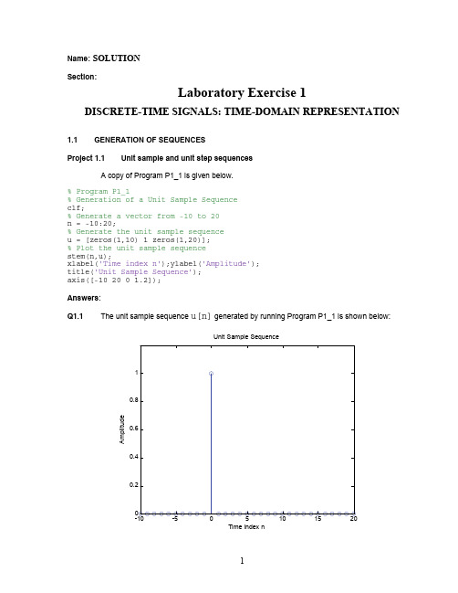
Name : SOLUTION Section :Laboratory Exercise 1DISCRETE-TIME SIGNALS: TIME-DOMAIN REPRESENTATION1.1GENERATION OF SEQUENCESProject 1.1Unit sample and unit step sequencesA copy of Program P1_1 is given below.% Program P1_1% Generation of a Unit Sample Sequence clf;% Generate a vector from -10 to 20 n = -10:20;% Generate the unit sample sequence u = [zeros(1,10) 1 zeros(1,20)]; % Plot the unit sample sequence stem(n,u);xlabel('Time index n');ylabel('Amplitude'); title('Unit Sample Sequence'); axis([-10 20 0 1.2]); Answers : Q1.1The unit sample sequence u[n] generated by running Program P1_1 is shown below:Time index nA m p l i t u d eUnit Sample SequenceQ1.2The purpose of clf command is – clear the current figureThe purpose of axis command is – control axis scaling and appearanceThe purpose of title command is – add a title to a graph or an axis and specify textpropertiesThe purpose of xlabel command is – add a label to the x-axis and specify textpropertiesThe purpose of ylabel command is – add a label to the y-axis and specify the textpropertiesQ1.3The modified Program P1_1 to generate a delayed unit sample sequence ud[n] with a delay of 11 samples is given below along with the sequence generated by running this program .% Program P1_1, MODIFIED for Q1.3% Generation of a DELAYED Unit Sample Sequence clf;% Generate a vector from -10 to 20 n = -10:20;% Generate the DELAYED unit sample sequence u = [zeros(1,21) 1 zeros(1,9)];% Plot the DELAYED unit sample sequence stem(n,u);xlabel('Time index n');ylabel('Amplitude'); title('DELAYED Unit Sample Sequence'); axis([-10 20 0 1.2]);Time index nA m p l i t u d eDELAYED Unit Sample SequenceQ1.4The modified Program P1_1 to generate a unit step sequence s[n] is given below along with the sequence generated by running this program .% Program Q1_4% Generation of a Unit Step Sequence clf;% Generate a vector from -10 to 20 n = -10:20;% Generate the unit step sequence s = [zeros(1,10) ones(1,21)]; % Plot the unit step sequence stem(n,s);xlabel('Time index n');ylabel('Amplitude'); title('Unit Step Sequence'); axis([-10 20 0 1.2]);Time index nA m p l i t u d eUnit Step SequenceQ1.5The modified Program P1_1 to generate a unit step sequence sd[n] with an advance of 7 samples is given below along with the sequence generated by running this program .% Program Q1_5% Generation of an ADVANCED Unit Step Sequence clf;% Generate a vector from -10 to 20 n = -10:20;% Generate the ADVANCED unit step sequence sd = [zeros(1,3) ones(1,28)];% Plot the ADVANCED unit step sequence stem(n,sd);xlabel('Time index n');ylabel('Amplitude'); title('ADVANCED Unit Step Sequence'); axis([-10 20 0 1.2]);Time index nA m p l i t u d eADVANCED Unit Step SequenceProject 1.2 Exponential signalsA copy of Programs P1_2 and P1_3 are given below .% Program P1_2% Generation of a complex exponential sequence clf;c = -(1/12)+(pi/6)*i; K = 2; n = 0:40;x = K*exp(c*n); subplot(2,1,1); stem(n,real(x));xlabel('Time index n');ylabel('Amplitude'); title('Real part'); subplot(2,1,2); stem(n,imag(x));xlabel('Time index n');ylabel('Amplitude'); title('Imaginary part');% Program P1_3% Generation of a real exponential sequence clf;n = 0:35; a = 1.2; K = 0.2; x = K*a.^n; stem(n,x);xlabel('Time index n');ylabel('Amplitude');Answers: Q1.6The complex-valued exponential sequence generated by running Program P1_2 is shown below :510152025303540Time index n A m p l i t u d eReal partTime index nA m p l i t u d eImaginary partQ1.7The parameter controlling the rate of growth or decay of this sequence is – the real part of c .The parameter controlling the amplitude of this sequence is - KQ1.8The result of changing the parameter c to (1/12)+(pi/6)*i is – since exp(-1/12) isless than one and exp(1/12) is greater than one, this change means that the envelope of the signal will grow with n instead of decay with n.Q1.9The purpose of the operator real is – to extract the real part of a Matlab vector.The purpose of the operator imag is – to extract the imaginary part of a Matlab vector. Q1.10The purpose of the command subplot is – to plot more than one graph in the sameMatlab figure.Q1.11The real-valued exponential sequence generated by running Program P1_3 is shown below :Time index nA m p l i t u d eQ1.12The parameter controlling the rate of growth or decay of this sequence is - aThe parameter controlling the amplitude of this sequence is - KQ1.13The difference between the arithmetic operators ^ and .^ is – “^” raises a square matrix toa power using matrix multiplication. “.^” raises the elements of a matrix or vector to a power; this is a “pointwise” operation.Q1.14The sequence generated by running Program P1_3 with the parameter a changed to 0.9 and the parameter K changed to 20 is shown below :5101520253035Time index nA m p l i t u d eQ1.15The length of this sequence is - 36It is controlled by the following MATLAB command line : n = 0:35;It can be changed to generate sequences with different lengths as follows (give an example command line and the corresponding length): n = 0:99; makes the length 100. Q1.16The energies of the real-valued exponential sequences x [n]generated in Q1.11 and Q1.14 and computed using the command sum are - 4.5673e+004 and 2.1042e+003.Project 1.3 Sinusoidal sequencesA copy of Program P1_4 is given below .% Program P1_4% Generation of a sinusoidal sequence n = 0:40;f = 0.1; phase = 0; A = 1.5; arg = 2*pi*f*n - phase; x = A*cos(arg);clf; % Clear old graphstem(n,x); % Plot the generated sequence axis([0 40 -2 2]); grid;title('Sinusoidal Sequence'); xlabel('Time index n'); ylabel('Amplitude'); axis; Answers:Q1.17 The sinusoidal sequence generated by running Program P1_4 is displayed below .0510152025303540Sinusoidal SequenceTime index nA m p l i t u d eQ1.18The frequency of this sequence is- f = 0.1 cycles/sample.It is controlled by the following MATLAB command line: f = 0.1;A sequence with new frequency 0.2 can be generated by the following command line:f = 0.2;The parameter controlling the phase of this sequence is- phaseThe parameter controlling the amplitude of this sequence is- AThe period of this sequence is - 2π/ω = 1/f = 10Q1.19 The length of this sequence is - 41It is controlled by the following MATLAB command line: n = 0:40;A sequence with new length __81_ can be generated by the following command line:n = 0:80;Q1.20 The average power of the generated sinusoidal sequence is–sum(x(1:10).*x(1:10))/10 = 1.1250Q1.21 The purpose of axis command is – to set the range of the x-axis to [0,40] and the range of the y-axis to [-2,2].The purpose of grid command is – to turn on the drawing of grid lines on the graph.Q1.22 The modified Program P1_4 to generate a sinusoidal sequence of frequency 0.9 is given below along with the sequence generated by running it.% Program Q1_22A% Generation of a sinusoidal sequencen = 0:40;f = 0.9;phase = 0;A = 1.5;arg = 2*pi*f*n - phase;x = A*cos(arg);clf; % Clear old graphstem(n,x); % Plot the generated sequenceaxis([0 40 -2 2]);grid;title('Sinusoidal Sequence');xlabel('Time index n');ylabel('Amplitude');axis;Sinusoidal SequenceTime index nA m p l i t u d eA comparison of this new sequence with the one generated in Question Q1.17 shows - thetwo graphs are identical. This is because, in the modified program, we have ω = 0.9*2π. This generates the same graph as a cosine with angular frequency ω - 2π = −0.1*2π. Because cosine is an even function, this is the same as a cosine with angular frequency +0.1*2π, which was the value used in P1_4.m in Q1.17.In terms of Hertzian frequency, we have for P1_4.m in Q1.17 that f = 0.1 Hz/sample. For the modified program in Q1.22, we have f = 0.9 Hz/sample, which generates the same graph as f = 0.9 – 1 = −0.1. Again because cosine is even, this makes a graph that is identical to the one we got in Q1.17 with f = +0.1 Hz/sample.A sinusoidal sequence of frequency 1.1 generated by modifying Program P1_4 is shown below.0510152025303540Sinusoidal SequenceTime index nA m p l i t u d eA comparison of this new sequence with the one generated in Question Q1.17 shows - thegraph here is again identical to the one in Q1.17. This is because a cosine of frequency f = 1.1 Hz/sample is identical to one with frequency f = 1.1 – 1 = 0.1 Hz/sample, which was the frequency used in Q1.17.Q1.23The sinusoidal sequence of length 50, frequency 0.08, amplitude 2.5, and phase shift of 90 degrees generated by modifying Program P1_4 is displayed below .NOTE: for this program, it is necessary to convert the phase of 90 deg to radians and account for the minus sign that appears in the statement “arg = 2*pi*f*n - phase;” as opposed to the plus sign shown in eq. (1.12) of the lab manual. The correct statement to generate the phase is “phase = -90/(2*pi);”. It is also necessary to modify the axis command to account for the new length and amplitude of the signal. The correct axis statement is “axis([0 50 -3 3]);”.05101520253035404550Sinusoidal SequenceTime index nA m p l i t u d eThe period of this sequence is - 2π/ω = 1/f = 1/0.08 = 1/(8/100) = 100/8 = 25/2.Therefore, the fundamental period is 25 and the graph has the “appearance” of going through 2 cycles of a cosine waveform during each period.Q1.24By replacing the stem command in Program P1_4 with the plot command, the plot obtained is as shown below :Sinusoidal SequenceTime index nA m p l i t u d eThe difference between the new plot and the one generated in Question Q1.17 is – instead ofdrawing stems from the x-axis to the points on the curve, the “plot ” command connects the points with straight line segments, which approximates the graph of a continuous-time cosine signal.Q1.25By replacing the stem command in Program P1_4 with the stairs command the plot obtained is as shown below :Sinusoidal SequenceTime index nA m p l i t u d eThe difference between the new plot and those generated in Questions Q1.17 and Q1.24 is– the “stairs” command produces a stairstep plot as opposed to the stem graph that was generated in Q1.17 and the straight-line interpolation plot that was generated in Q1.24.Project 1.4 Random signalsAnswers:Q1.26 The MATLAB program to generate and display a random signal of length 100 with elements uniformly distributed in the interval [–2, 2] is given below along with the plot of the random sequence generated by running the program:% Program Q1_26% Generation of a uniform random sequencen = 0:99;A = 2;rand('state',sum(100*clock)); % "seed" the generator% rand(1,100) is uniform in [0,1]% rand(1,100)-0.5 is uniform in [-0.5,0.5]% 4*(rand(1,100)-0.5) is uniform in [-2,2]x = 2*A*(rand(1,length(n))-0.5);clf; % Clear old graphstem(n,x); % Plot the generated sequenceaxis([0 length(n) -round(2*(A+0.5))/2 round(2*(A+0.5))/2]);grid;title('Uniform Random Sequence');xlabel('Time index n');ylabel('Amplitude');axis;102030405060708090100Uniform Random SequenceTime index nA m p l i t u d eQ1.27 The MATLAB program to generate and display a Gaussian random signal of length 75 withelements normally distributed with zero mean and a variance of 3 is given below along with the plot of the random sequence generated by running the program :% Program Q1_27% Generation of a Gaussian random sequence% NOTE: if X is a random variable with zero mean and % unity variance, then (aX + b) is a random variable % with mean b and variance a^2. This follows from % basic probability theory. n = 0:74;xmean = 0; % mean of xxstd = sqrt(3); % standard deviation of xrandn('state',sum(100*clock)); % "seed" the generator % generate the sequencex = xstd*randn(1,length(n)) + xmean; % setup the graph and plotclf; % Clear old graphstem(n,x); % Plot the generated sequence xmax = max(abs(x));Ylim = round(2*(xmax+0.5))/2; axis([0 length(n) -Ylim Ylim]); grid;title('Gaussian Random Sequence'); xlabel('Time index n'); ylabel('Amplitude'); axis;10203040506070Gaussian Random SequenceTime index nA m p l i t u d eQ1.28The MATLAB program to generate and display five sample sequences of a random sinusoidal signal of length 31{X[n]} = {A·cos(ωo n + φ)}where the amplitude A and the phase φ are statistically independent random variables with uniform probability distribution in the range 0≤A ≤4 for the amplitude and in the range 0 ≤ φ ≤ 2π for the phase is given below. Also shown are five sample sequences generated by running this program five different times .% Generates the "deterministic stochastic process" % called for in Q1.28. n = 0:30; f = 0.1; Amax = 4;phimax = 2*pi;rand('state',sum(100*clock)); % "seed" the generator A = Amax*rand;% NOTE: successive calls to rand without arguments % return a random sequence of scalars. Since this % random sequence is "white" (uncorrelated), it is % not necessary to re-seed the generator for phi. phi = phimax*rand;% generate the sequence arg = 2*pi*f*n + phi; x = A*cos(arg); % plotclf; % Clear old graphstem(n,x); % Plot the generated sequence Ylim = round(2*(Amax+0.5))/2; axis([0 length(n) -Ylim Ylim]); grid;title('Sinusoidal Sequence with Random Amplitude and Phase'); xlabel('Time index n'); ylabel('Amplitude'); axis;Sinusoidal Sequence with Random Amplitude and PhaseTime index nA m p l i t u d eSinusoidal Sequence with Random Amplitude and PhaseTime index nA m p l i t u d eTime index nA m p l i t u d eSinusoidal Sequence with Random Amplitude and PhaseTime index nA m p l i t u d eTime index nA m p l i t u d e1.2 SIMPLE OPERATIONS ON SEQUENCESProject 1.5Signal SmoothingA copy of Program P1_5 is given below .% Program P1_5% Signal Smoothing by Averaging clf; R = 51;d = 0.8*(rand(R,1) - 0.5); % Generate random noise m = 0:R-1;s = 2*m.*(0.9.^m); % Generate uncorrupted signal x = s + d'; % Generate noise corrupted signal subplot(2,1,1);plot(m,d','r-',m,s,'g--',m,x,'b-.');xlabel('Time index n');ylabel('Amplitude'); legend('d[n] ','s[n] ','x[n] ');x1 = [0 0 x];x2 = [0 x 0];x3 = [x 0 0]; y = (x1 + x2 + x3)/3; subplot(2,1,2);plot(m,y(2:R+1),'r-',m,s,'g--'); legend( 'y[n] ','s[n] ');xlabel('Time index n');ylabel('Amplitude'); Answers: Q1.29The signals generated by running Program P1_5 are displayed below :05101520253035404550-5510Time index nA m p l i t u d e2468Time index nA m p l i t u d eQ1.30The uncorrupted signal s[n]is - the product of a linear growth with a slowly decayingreal exponential.The additive noise d[n]is – a random sequence uniformly distributed between -0.4 and+0.4.Q1.31 The statement x = s + d CANNOT be used to generate the noise corrupted signalbecause – d is a column vector, whereas s is a row vector; it is necessary to transposeone of these vectors before adding them.Q1.32The relations between the signals x1, x2, and x3, and the signal x are – all three signalsx1, x2, and x3 are extended versions of x , with one additional sample appended at the left and one additional sample appended to the right. The signal x1 is a delayedversion of x , shifted one sample to the right with zero padding on the left. The signal x2 is equal to x , with equal zero padding on both the left and right to account for the extended length. Finally, x3 is a time advanced version of x , shifted one sample to the left with zero padding on the right.Q1.33The purpose of the legend command is – to create a legend for the graphs. In P1_5, the signals are plotted using different colors and line types; the legend providesinformation about which color and line type is associated with each signal.Project 1.6Generation of Complex SignalsA copy of Program P1_6 is given below.% Program P1_6% Generation of amplitude modulated sequenceclf;n = 0:100;m = 0.4;fH = 0.1; fL = 0.01;xH = sin(2*pi*fH*n);xL = sin(2*pi*fL*n);y = (1+m*xL).*xH;stem(n,y);grid;xlabel('Time index n');ylabel('Amplitude');Answers:Q1.34 The amplitude modulated signals y[n]generated by running Program P1_6 for various values of the frequencies of the carrier signal xH[n]and the modulating signal xL[n], andvarious values of the modulation index m are shown below:m=0.4; fH=0.1; fL=0.01:Time index nA m p l i t u d em=0.9; fH=0.1; fL=0.1:Time index nA m p l i t u d em=0.4; fH=0.1; fL=0.005:Time index nA m p l i t u d em=0.4; fH=0.25; fL=0.01:Time index nA m p l i t u d eQ1.35 The difference between the arithmetic operators * and .* is – “*” multiplies twoconformable matrices or vectors using matrix multiplication. “.*” takes the pointwise products of the elements of two matrices or vectors that have the same dimensions.A copy of Program P1_7 is given below .% Program P1_7% Generation of a swept frequency sinusoidal sequence n = 0:100; a = pi/2/100; b = 0;arg = a*n.*n + b*n; x = cos(arg);clf; stem(n, x);axis([0,100,-1.5,1.5]);title('Swept-Frequency Sinusoidal Signal'); xlabel('Time index n'); ylabel('Amplitude'); grid; axis; Answers:Q1.36 The swept-frequency sinusoidal sequence x[n] generated by running Program P1_7 isdisplayed below .Swept-Frequency Sinusoidal SignalTime index nA m p l i t u d eQ1.37The minimum and maximum frequencies of this signal are - The minimum occurs at n=0, where we have 2an+b = 0 rad/sample = 0 Hz/sample. The maximum occurs at n=100, where we have 2an+b = 200a = 200π(0.5)(0.01) = π rad/sample= 0.5 Hz/sample.Q1.38The Program 1_7 modified to generate a swept sinusoidal signal with a minimum frequency of0.1 and a maximum frequency of 0.3 is given below:Note: for a minimum frequency of 0.1 Hz/sample = π/5 rad/sample at n=0, we must have 2a(0) + b =π/5, which implies b=π/5. For a maximum frequency of 0.3 Hz/sample = 3π/5 rad/sample at n=100, we must have 2a(100) + π/5 = 3π/5, which implies a=π/500.% Program Q1_38% Generation of a swept frequency sinusoidal sequencen = 0:100;a = pi/500;b = pi/5;arg = a*n.*n + b*n;x = cos(arg);clf;stem(n, x);axis([0,100,-1.5,1.5]);title('Swept-Frequency Sinusoidal Signal');xlabel('Time index n');ylabel('Amplitude');grid; axis;INFORMATION1.3 WORKSPACEQ1.39The information displayed in the command window as a result of the who command is – a listing of the names of the variables defined in the current workspace.Q1.40The information displayed in the command window as a result of the whos command is – a long form listing of the variables defined in the current workspace, including the variable names, their dimensions (size), the number of bytes of storage required for each variable, and the datatype of each variable. The total number of bytes of storagefor the entire workspace is also displayed.1.4 OTHER TYPES OF SIGNALS (Optional)Project 1.8 Squarewave and Sawtooth SignalsAnswer:Q1.41MATLAB programs to generate the square-wave and the sawtooth wave sequences of the type shown in Figures 1.1 and 1.2 are given below along with the sequences generated by running these programs:% Program Q1_41A% Generation of the square wave in Fig. 1.1(a)n = 0:30;f = 0.1;phase = 0;duty=60;A = 2.5;arg = 2*pi*f*n + phase;x = A*square(arg,duty);clf; % Clear old graphstem(n,x); % Plot the generated sequenceaxis([0 30 -3 3]);grid;title('Square Wave Sequence of Fig. 1.1(a)');xlabel('Time index n');ylabel('Amplitude');axis;% Program Q1_41B% Generation of the square wave in Fig. 1.1(b)n = 0:30;f = 0.1;phase = 0;duty=30;A = 2.5;arg = 2*pi*f*n + phase;x = A*square(arg,duty);clf; % Clear old graphstem(n,x); % Plot the generated sequenceaxis([0 30 -3 3]);grid;title('Square Wave Sequence of Fig. 1.1(b)');xlabel('Time index n');ylabel('Amplitude');axis;% Program Q1_41C% Generation of the square wave in Fig. 1.2(a) n = 0:50;f = 0.05;phase = 0;peak = 1;A = 2.0;arg = 2*pi*f*n + phase;x = A*sawtooth(arg,peak);clf; % Clear old graphstem(n,x); % Plot the generated sequence axis([0 50 -2 2]);grid;title('Sawtooth Wave Sequence of Fig. 1.2(a)'); xlabel('Time index n');ylabel('Amplitude');axis;% Program Q1_41D% Generation of the square wave in Fig. 1.2(b) n = 0:50;f = 0.05;phase = 0;peak = 0.5;A = 2.0;arg = 2*pi*f*n + phase;x = A*sawtooth(arg,peak);clf; % Clear old graphstem(n,x); % Plot the generated sequence axis([0 50 -2 2]);grid;title('Sawtooth Wave Sequence of Fig. 1.2(b)'); xlabel('Time index n');ylabel('Amplitude');axis;051015202530Time index nA m p l i t u d eSquare Wave Sequence of Fig. 1.1(b)Time index nA m p l i t u d eTime index nA m p l i t u d eSawtooth Wave Sequence of Fig. 1.2(b)Time index nA m p l i t u d eDate: 14 September, 2006 Signature: HAVLICEK。
数字信号处理教程第四版答案

z2 x (n ) [z ]z 0 8 1 (z )z 4
当n 0时,围线内部没有极点 ,故x(n) 0
1 x(n) 7 u(n 1) 8(n) 4
n
z2 部分分式法: X(z) 1 z 4 X(z) z2 A1 A2 故 1 1 z z (z )z z 4 4
数 字 信 号 处 理
第二章 z变换与离散时间傅里叶 变换(DTFT)
2.2 z变换的定义与收敛域
序列x(ห้องสมุดไป่ตู้)的z变换定义为:
n x ( n ) z
X ( z)
n
对任意给定序列x(n),使其z变换收敛的所有z值的集合 称为X(z)的收敛域,上式收敛的充分必要条件是满足绝 对可和
1 z2 A1 [(z ) ] 1 7 1 4 (z )z z 4 4 z2 A 2 [z ] 8 1 z 0 (z )z 4
n
7 1 X( z ) 8,| z | 1 1 4 1 z 4
1 x(n) 7 u(n 1) 8(n) 4
1 | z | 4
n 1
jIm[z]
1/4 o
Re[z]
当n 1时,分母中z的阶次比分子中 z的阶次高两阶 或两阶以上,可用围线 外部极点求解
1 (z 2)z n 1 1 n x (n ) [(z ) ] 1 7( ) z 1 4 4 4 z 4
z2 当n 0时,F(z) ,此时围线内部有一阶 极点z 0 1 (z )z 4
1 n x (n ) ( ) u (n ) 2
部分分式法: Z[a n u (n )]
1 , | z || a | 1 1 az
数字信号处理—原理、实现及应用(第4版)第8章 时域离散系统的实现 学习要点及习题答案
·185·第8章 时域离散系统的实现本章学习要点第8章研究数字信号处理系统的实现方法。
数字信号处理系统设计完成后得到的是该系统的系统函数或者差分方程,要实现还需要设计一种具体的算法,这些算法会影响系统的成本以及运算误差等。
本章介绍常用的几种系统结构,即系统算法,同时简明扼要地介绍数字信号处理中的量化效应,最后介绍了MA TLAB 语言中的滤波器设计和分析工具。
本章学习要点如下:(1) 由系统流图写出系统的系统函数或者差分方程。
(2) 按照FIR 系统的系统函数或者差分方程画出其直接型、级联型和频率采样结构,FIR 线性相位结构,以及用快速卷积法实现FIR 系统。
(3) 按照IIR 系统的系统函数或者差分方程画出其直接型、级联型、并联型。
(4) 一般了解格型网络结构,包括全零点格型网络结构系统函数、由FIR 直接型转换成全零点格型网络结构、全极点格型网络结构及其系统函数。
(5) 一般了解如何用软件实现各种网络结构,并排出运算次序。
(6) 数字信号处理中的量化效应,包括A/D 变换器中的量化效应、系数量化效应、运算中的量化效应及其影响。
(7) 了解用MA TLAB 语言设计、分析滤波器。
8.5 习题与上机题解答8.1 已知系统用下面差分方程描述311()(1)(2)()(1)483y n y n y n x n x n =---++- 试分别画出系统的直接型、级联型和并联型结构。
差分方程中()x n 和()y n 分别表示系统的输入和输出信号。
解:311()(1)(2)()(1)483y n y n y n x n x n --+-=+- 将上式进行Z 变换,得到121311()()()()()483Y z Y z z Y z z X z X z z ----+=+ 112113()31148z H z z z ---+=-+ (1) 按照系统函数()H z ,画出直接型结构如图S8.1.1所示。
数字信号处理—原理、实现及应用(第4版)第4章 模拟信号数字处理 学习要点及习题答案
·78· 第4章 模拟信号数字处理4.1 引 言模拟信号数字处理是采用数字信号处理的方法完成模拟信号要处理的问题,这样可以充分利用数字信号处理的优点,本章也是数字信号处理的重要内容。
4.2 本章学习要点(1) 模拟信号数字处理原理框图包括预滤波、模数转换、数字信号处理、数模转换以及平滑滤波;预滤波是为了防止频率混叠,模数转换和数模转换起信号类型匹配转换作用,数字信号处理则完成对信号的处理,平滑滤波完成对数模转换后的模拟信号的进一步平滑作用。
(2) 时域采样定理是模拟信号转换成数字信号的重要定理,它确定了对模拟信号进行采样的最低采样频率应是信号最高频率的两倍,否则会产生频谱混叠现象。
由采样得到的采样信号的频谱和原模拟信号频谱之间的关系式是模拟信号数字处理重要的公式。
对带通模拟信号进行采样,在一定条件下可以按照带宽两倍以上的频率进行采样。
(3) 数字信号转换成模拟信号有两种方法,一种是用理想滤波器进行的理想恢复,虽不能实现,但没有失真,可作为实际恢复的逼近方向。
另一种是用D/A 变换器,一般用的是零阶保持器,虽有误差,但简单实用。
(4) 如果一个时域离散信号是由模拟信号采样得来的,且采样满足采样定理,该时域离 散信号的数字频率和模拟信号的模拟频率之间的关系为T ωΩ=,或者s /F ωΩ=。
(5) 用数字网络从外部对连续系统进行模拟,数字网络的系统函数和连续系统传输函数 之间的关系为j a /(e )(j )T H H ωΩωΩ==,≤ωπ。
数字系统的单位脉冲响应和模拟系统的单位冲激响应关系应为 a a ()()()t nTh n h t h nT === (6) 用DFT (FFT )对模拟信号进行频谱分析(包括周期信号),应根据时域采样定理选择采样频率,按照要求的分辨率选择观测时间和采样点数。
要注意一般模拟信号(非周期)的频谱是连续谱,周期信号是离散谱。
用DFT (FFT )对模拟信号进行频谱分析是一种近似频谱分析,但在允许的误差范围内,仍是很重要也是常用的一种分析方法。
数字信号处理—原理、实现及应用(第4版)第3章 离散傅里叶变换及其快速算法 学习要点及习题答案

·54· 第3章 离散傅里叶变换(DFT )及其快速算法(FFT )3.1 引 言本章是全书的重点,更是学习数字信号处理技术的重点内容。
因为DFT (FFT )在数字信号处理这门学科中起着不一般的作用,它使数字信号处理不仅可以在时域也可以在频域进行处理,使处理方法更加灵活,能完成模拟信号处理完不成的许多处理功能,并且增加了若干新颖的处理内容。
离散傅里叶变换(DFT )也是一种时域到频域的变换,能够表征信号的频域特性,和已学过的FT 和ZT 有着密切的联系,但是它有着不同于FT 和ZT 的物理概念和重要性质。
只有很好地掌握了这些概念和性质,才能正确地应用DFT (FFT ),在各种不同的信号处理中充分灵活地发挥其作用。
学习这一章重要的是会应用,尤其会使用DFT 的快速算法FFT 。
如果不会应用FFT ,那么由于DFT 的计算量太大,会使应用受到限制。
但是FFT 仅是DFT 的一种快速算法,重要的物理概念都在DFT 中,因此重要的还是要掌握DFT 的基本理论。
对于FFT 只要掌握其基本快速原理和使用方法即可。
3.2 习题与上机题解答说明:下面各题中的DFT 和IDFT 计算均可以调用MA TLAB 函数fft 和ifft 计算。
3.1 在变换区间0≤n ≤N -1内,计算以下序列的N 点DFT 。
(1) ()1x n =(2) ()()x n n δ=(3) ()(), 0<<x n n m m N δ=- (4) ()(), 0<<m x n R n m N = (5) 2j()e, 0<<m n N x n m N π=(6) 0j ()e n x n ω=(7) 2()cos , 0<<x n mn m N N π⎛⎫= ⎪⎝⎭(8)2()sin , 0<<x n mn m N N π⎛⎫= ⎪⎝⎭(9) 0()cos()x n n ω=(10) ()()N x n nR n =(11) 1,()0n x n n ⎧=⎨⎩,解:(1) X (k ) =1N kn N n W -=∑=21j0eN kn nn π--=∑=2jj1e1ekN n k nπ---- = ,00,1,2,,1N k k N =⎧⎨=-⎩(2) X (k ) =1()N knNM n W δ-=∑=10()N n n δ-=∑=1,k = 0, 1, …, N -1(3) X (k ) =100()N knNn n n W δ-=-∑=0kn NW 1()N n n n δ-=-∑=0kn NW,k = 0, 1, …, N -1为偶数为奇数·55·(4) X (k ) =1m knN n W -=∑=11kmN N W W --=j (1)sin esin k m N mk N k N π--π⎛⎫⎪⎝⎭π⎛⎫ ⎪⎝⎭,k = 0, 1, …, N -1 (5) X (k ) =21j 0e N mn kn N N n W π-=∑=21j ()0e N m k nNn π--=∑=2j()2j()1e1em k N N m k Nπ--π----= ,0,,0≤≤1N k mk m k N =⎧⎨≠-⎩(6) X (k ) =01j 0eN nknN n W ω-=∑=021j 0e N k nN n ωπ⎛⎫-- ⎪⎝⎭=∑=002j 2j 1e1ek NN k N ωωπ⎛⎫- ⎪⎝⎭π⎛⎫- ⎪⎝⎭--= 0210j 202sin 2e2sin /2N k N N k N k N ωωωπ-⎛⎫⎛⎫- ⎪⎪⎝⎭⎝⎭⎡⎤π⎛⎫- ⎪⎢⎥⎝⎭⎣⎦⎡⎤π⎛⎫- ⎪⎢⎥⎝⎭⎣⎦,k = 0, 1, …, N -1或 X (k ) =00j 2j 1e 1e Nk N ωωπ⎛⎫- ⎪⎝⎭--,k = 0, 1, …, N -1(7) X (k ) =102cos N kn N n mn W N -=π⎛⎫ ⎪⎝⎭∑=2221j j j 01e e e 2N mn mn kn N N N n πππ---=⎛⎫ ⎪+ ⎪⎝⎭∑=21j ()01e 2N m k n N n π--=∑+21j ()01e 2N m k n N n π--+=∑=22j ()j ()22j ()j ()11e 1e 21e 1e m k N m k N N N m k m k N N ππ--+ππ--+⎡⎤--⎢⎥+⎢⎥⎢⎥--⎣⎦=,,20,,N k m k N mk m k N M ⎧==-⎪⎨⎪≠≠-⎩,0≤≤1k N - (8) ()22j j 21()sin ee 2j mn mnN N x n mn N ππ-π⎛⎫== ⎪-⎝⎭ ()()112222j j j ()j ()0011()=e e ee 2j 2j j ,2=j ,20,(0≤≤1)N N kn mn mn m k n m k n N N N N N n n X k W Nk m N k N mk k N --ππππ---+===--⎧-=⎪⎪⎨=-⎪⎪-⎪⎩∑∑其他(9) 解法① 直接计算χ(n ) =cos(0n ω)R N (n ) =00j j 1[e e ]2n n ωω-+R N (n )X (k ) =1()N knNn n W χ-=∑=0021j j j 01[e e ]e 2N kn n n N n ωωπ---=+∑=0000j j 22j j 11e 1e 21e 1e N N k k N N ωωωω-ππ⎛⎫⎛⎫--+ ⎪ ⎪⎝⎭⎝⎭⎡⎤--⎢⎥+⎢⎥⎢⎥--⎣⎦,k = 0, 1, … , N -1 解法② 由DFT 共轭对称性可得同样的结果。
数字信号处理实验4答案.docx

一、实验目的深刻理解离散时间系统的系统函数在分析离散系统的时域特性、频域特性以及稳定性中的重要作用及意义,熟练掌握利用MATLAB分析离散系统的时域响应、频响特性和零极点的方法。
掌握利用DTFT和DFT 确定系统特性的原理和方法。
二、实验原理MATLAB提供了许多可用于分析线性时不变连续系统的函数,主要包含有系统函数、系统时域响应、系统频域响应等分析函数。
1.离散系统的时域响应2.离散系统的系统函数零极点分析3.离散系统的频率响应4.利用DTFT和DFT确定离散系统的特性三、实验内容1.已知某LTI系统的差分方程为:尹[妇-1. 143尹顷一1] + 0. 412尹- 2]=0. 0675x[妇 + 0. 1349x[A - 1] + 0. 0675x[A - 2]1.初始状态y[-1] = 1, y[-2] = 2,输入= 〃伏]计算系统的完全响应.程序:a=[l,-1.143,0.412];b=[O.O675,0.1349,0.0675];n=40;x=ones(l,n);yi=[l,2];zi=filtic(b,a,yi);y=filter(b,a,x,zi);stem(y)(2)当以下三个信号分别通过系统时,分别计算离散系统的零状态响应:X』妇=cos (—; xS_k\ = cos (—= cos (—10 5 10程序n=100;k=0:n-1;a=[l,-1.143,0.412];b=[0.0675,0.1349,0.0675];xl=cos(pi*k/10);x2 = cos (pi*k/5);x3=cos(7*pi*k/10);yl=filter(b,a,xl);y2=filter(b,a,x2);y3=filter(b,a,x3);subplot(3,1,1);stem(k, yl) subplot(3,1,2); stem(k,y2)subplot(3,1,3); stem(k,y3)10 20 30 40 50 60 70 80 90 1002. 已知某因果LTI 系统的系统函数为:m 、0. 03571 + 0. 1428/T + 0. 2143z~2 + 0. 1428z~3 + 0.0357lz~4 H(z) = -------- - ------- § ----------------------- ------------------------------- 7 -------- 1 - 1. 035/T + 0. 8264/2 — Q. 2605/3 + o. 04033z~4 (1) 计算系统的单位脉冲响应。
数字信号处理_习题与解答

[ax (k ) bx (k )]
1 2 2 1 2
x1( k ) b
n n0
k n n0
x (k ) aT[ x (n)] bT[ x (n)]
系统是线性系统 9
( 4)T [ x( n )] x( n n0) ( a )若 | x( n ) | M ,则: | T [ x( n )] || x( n n0 ) | M 系统是稳定系统 (b ) y( n ) x( n n0 ), (i )n0 0, n n0 n, y( n )与n时刻之后的输入无关 系统是因果系统 (ii )n0 0, n n0 n, y( n )与n时刻之后的输入有关 系统不是因果系统 (c ) T [ax1( n ) bx2 ( n )] ax1( n n0 ) bx2 ( n n0 ) aT[ x1( n )] bT[ x2 ( n )] 系统是稳定系统
15
1 2 j n x( n ) X ( j )e d 2 0 1 2 j 2 n x ( 2n ) X ( j )e d 2 0 1 4 j ' n X ( j '/ 2)e d ' ( ' 2) 4 0 1 2 j n 1 4 j n X ( j )e d X ( j )e d 4 0 2 4 2 2 1 2 j n 1 2 2 j n X ( j )e d X( j )e d 2 0 2 4 0 2 2 1 2 1 j n [ X ( j ) X [ j ( )]e d G ( j )e j d 0 0 2 2 2 2 16
数字信号处理-基于计算机的方法(第四版)答案 8-11章
Copyright © 2011 by Sanjit K. Mitra. No part of this publication may be reproduced or distributed in any form or by any means, or stored in a database or retrieval system, without the prior written consent of Sanjit K. Mitra, including, but not limited to, in any network or other electronic Storage or transmission, or broadcast for distance learning.
D = 2〈2−1 〉 5 = 6.
€
€
⎧0 ≤ n1 ≤ 4, Thus, n = 〈5 n1 + 2 n 2 〉10 , ⎨ ⎩0 ≤ n 2 ≤ 2, ⎧0 ≤ k ≤ 4, k = 〈5 k1 + € 6 k 2 〉10 , ⎨ €1 ⎩0 ≤ k 2 ≤ 2. The corresponding€ index mappings are indicated below:
- 1、下载文档前请自行甄别文档内容的完整性,平台不提供额外的编辑、内容补充、找答案等附加服务。
- 2、"仅部分预览"的文档,不可在线预览部分如存在完整性等问题,可反馈申请退款(可完整预览的文档不适用该条件!)。
- 3、如文档侵犯您的权益,请联系客服反馈,我们会尽快为您处理(人工客服工作时间:9:00-18:30)。
Laboratory Exercise 4
LINEAR, TIME-INVARIANT DISCRETE-TIME SYSTEMS: FREQUENCY-DOMAIN REPRESENTATIONS
4.1 TRANSFER FUNCTION AND FREQUENCY RESPONSE
M=3
Magnitude Spectrum |H(ej)| 1
0.5
0 0 0.2 0.4 0.6 0.8 1 1.2 1.4 1.6 1.8 2 / Phase Spectrum arg[H(ej)]
4 2 0 -2 -4
0 0.2 0.4 0.6 0.8 1 1.2 1.4 1.6 1.8 2 /
I shall choose the filter of Question Q4._36__ for the following reason - It can be both causal and BIBO stable, whereas the filter of Q4.37 cannot be both because the two poles are both outside of the unit circle.
Q4.5
The plots of the first 100 samples of the impulse responses of the two filters of Questions 4.2
2
Amplitude
Phase in radians
Amplitude
Phase in radians
M=10
Magnitude Spectrum |H(ej)| 1
0.5
0 0 0.2 0.4 0.6 0.8 1 1.2 1.4 1.6 1.8 2 / Phase Spectrum arg[H(ej)]
4 2 0 -2 -4
0 0.1 0.2 0.3 0.4 0.5 0.6 0.7 0.8 0.9 1 /
The type of filter represented by this transfer function is - Bandpass
The difference between the two filters of Questions 4.2 and 4.3 is - The magnitude responses are the same. The phase responses might look very different to you at first,
1
Amplitude
Phase in radians
This program was run for the following three different values of M and the plots of the corresponding frequency responses are shown below:
Q4.4
The group delay of the filter specified in Question Q4.4 and obtained using the function
grpdelay is shown below:
Group Delay of H(ej) 7
6
5
4Leabharlann group delay3
Q4.2
The plot of the frequency response of the causal LTI discrete-time system of Question Q4.2
obtained using the modified program is given below:
Magnitude Spectrum |H(ej)| 1
M=7
Magnitude Spectrum |H(ej)| 1
0.5
0 0 0.2 0.4 0.6 0.8 1 1.2 1.4 1.6 1.8 2 / Phase Spectrum arg[H(ej)]
4 2 0 -2 -4
0 0.2 0.4 0.6 0.8 1 1.2 1.4 1.6 1.8 2 /
Project 4.1 Transfer Function Analysis
Answers:
Q4.1
The modified Program P3_1 to compute and plot the magnitude and phase spectra of a moving
average filter of Eq. (2.13) for 0 2 is shown below:
Amplitude
0.5
Phase in radians
0 0 0.1 0.2 0.3 0.4 0.5 0.6 0.7 0.8 0.9 1 / Phase Spectrum arg[H(ej)]
2
1
0
-1
-2 0 0.1 0.2 0.3 0.4 0.5 0.6 0.7 0.8 0.9 1 /
Q4.3
4 2 0 -2 -4
0 0.2 0.4 0.6 0.8 1 1.2 1.4 1.6 1.8 2 /
The types of symmetries exhibited by the magnitude and phase spectra are due to - The impulse response is real. Therefore, the frequency response is periodically conjugate symmetric, the magnitude response is periodically even symmetric, and the phase response is periodically odd symmetric. The type of filter represented by the moving average filter is - This is a lowpass filter. The results of Question Q2.1 can now be explained as follows – It is a lowpass filter. The input was a sum of two sinusoids, one high frequency and one low frequency. The particular results depend on the filter length M, but the general result is that the higher frequency sinusoidal input component is attenuated more than the lower frequency sinusoidal input component.
The type of filter represented by this transfer function is - Bandpass
The plot of the frequency response of the causal LTI discrete-time system of Question Q4.3
% Program Q4_1 % Frequency response of the causal M-point averager of Eq. (2.13) clear; % User specifies filter length M = input('Enter the filter length M: '); % Compute the frequency samples of the DTFT w = 0:2*pi/1023:2*pi; num = (1/M)*ones(1,M); den = [1]; % Compute and plot the DTFT h = freqz(num, den, w); subplot(2,1,1) plot(w/pi,abs(h));grid title('Magnitude Spectrum |H(e^{j\omega})|') xlabel('\omega /\pi'); ylabel('Amplitude'); subplot(2,1,2) plot(w/pi,angle(h));grid title('Phase Spectrum arg[H(e^{j\omega})]') xlabel('\omega /\pi'); ylabel('Phase in radians');
4
but they are actually similar. The phase response of the second filter exhibits a branch cut of the arctangent function at normalized frequency 0.4, which is right in the middle of the passband. However, the unwrapped phase would not show this discontinuity. Both filters have an approximately linear phase in the passband and their group delays are approximately the negatives of one another. However, the two filters have different poles. The poles of the first filter are INSIDE the unit circle, whereas those of the second filer are OUTSIDE the unit circle. Thus, in a causal implementation, the first filter would be BIBO STABLE, whereas the second filter would be UNSTABLE. Therefore, in most applications the second filter would be preferable.