SPSS加权最小二乘法及应用
spss最小二乘估计求回归方程

spss最小二乘估计求回归方程SPSS最小二乘估计求回归方程为标题,写一篇3000字的文章> SPSS最小二乘估计(Least Squares Estimation, LSE)是一种常用的统计回归分析方法,它可以用来求解回归方程,其关键步骤是将变量之间的关系以线性方程的形式表示,并使用最小二乘法将结果进行估计。
其中的参数可以用来描述回归方程的性质。
1. SPPS最小二乘估计的基本原理SPPS最小二乘估计(Least Squares Estimation, LSE)通过拟合数据点到一条直线,使得所有观测点到这条直线的残差平方和(residual sum of squares,RSS)最小,这样可以有效地拟合观测数据,从而可以确定回归方程。
为了确定回归方程,首先需要确定自变量和因变量之间的关系,记为:Y = 0 + 1 X 1 + 2 X 2 + + n X n其中,Y为因变量,X1,X2,…,Xn为自变量,β0,β1,…,βn为回归方程参数,它们需要求解,以便使得回归方程能够最大程度地拟合观测数据。
通过最小二乘估计求解的回归方程,有许多优点:首先,它可以得到准确的结果,即使模型中出现噪声,结果也是可靠的;其次,它具有较小的标准误差和较小的偏差,而且与观测数据紧密相关;最后,它可以用来分析两个或多个变量之间的相关关系,利用这些变量可以预测某一变量的值,并可以根据这些变量计算出模型参数,提高模型的准确性和精确性。
2. SPPS最小二乘估计的应用(1)营销领域:可以利用最小二乘估计的方法,分析营销中的投放力度,投放媒介,投放时间等因素与消费者购买行为之间的关系,分析出影响消费者购买行为的因素,并可以利用模型估计出投放参数,用以提高营销的效率。
(2)金融领域:利用最小二乘估计的方法,可以分析不同的股票或个股的走势,其中的变量有价格、成交量、利润率等,可以分析其中不同股票或个股之间的关系,为投资者提供参考。
SPSS教程:做多重线性回归,方差不齐怎么办

SPSS教程:做多重线性回归,方差不齐怎么办今天我们就来继续讨论一下,如果残差不满足方差齐性时,应该如何解决?一、残差方差齐性判断1. 残差方差齐性回顾一下前面介绍过的残差方差齐性,即残差ei的大小不随预测值水平的变化而变化。
我们在进行残差分析时,可以通过绘制标准化残差和标准化预测值的散点图来进行判断。
若残差满足方差齐性,则标准化残差的散点会在一定区域内,围绕标准化残差ei=0这条直线的上下两侧均匀分布,不随标准化预测值的变化而变化,如图1所示。
图1. 标准化残差散点图(方差齐性)2. 残差方差不齐但有时残差不满足方差齐性的假设,其标准化残差散点图显示,残差的变异程度随着变量取值水平的变化而发生变化,如图2(a)显示标准化残差的分布随变量取值的增大而呈现扩散趋势,图2(b)显示标准化残差的分布随变量取值的增大而呈现收敛趋势,说明残差不满足方差齐性的条件。
图2. 标准化残差散点图(方差不齐)二、加权最小二乘法在多重线性回归模型中,我们采用的是普通最小二乘法(Ordinary Least Square,OLS)来对参数进行估计,即要求每个观测点的实际值与预测值之间的残差平方和最小,对于模型中的每个观测点是同等看待的,残差满足方差齐性的假设。
但是在有些研究问题中,例如调查某种疾病的发病率,以地区为观测单位,很显然地区人数越多,所得到的率就越稳定,变异程度越小,而地区人数越少,所得到的率的变异就越大。
在这种情况下,因变量的变异程度会随着自身数值或其他变量的变化而变化,残差不满足方差齐性的条件。
此时如果继续采用OLS方法进行模型估计,则拟合结果就会受到变异程度较大的数据的影响,在这种情况下构建的回归模型就会发生偏差,预测精度降低,甚至预测功能失效。
为了解决这一问题,我们可以采用加权最小二乘法(Weighted Least Squares,WLS)的方法来进行模型估计,即在模型拟合时,根据数据变异程度的大小赋予不同的权重,对于变异程度较小、测量更精确的数据赋予较大的权重,对于变异程度较大、测量不稳定的数据赋予较小的权重,从而使得加权后回归直线的残差平方和最小,保证拟合的模型具有更好的预测价值。
薛薇,《SPSS统计分析方法及应用》第八章 相关分析和线性回归分析

以控制,进行偏相关分析。
偏相关分 析输出结 果;负的 弱相关
相关分析 输出结果 ;正强相 关
8.4.1
8.4.2
回归分析概述
线性回归模型
8.4.3
8.4.4 8.4.5 8.4.6
回归方程的统计检验
基本操作
其它操作
应用举例
线性回归分析的内容
能否找到一个线性组合来说明一组自变量和因变量
可解释x对Y的影响大小,还可 以对y进行预测与控制
目的是刻画变量间的相关 程度
8.2.1 8.2.2 8.2.3 8.2.4
散点图 相关系数 基本操作 应用举例
•
相关分析通过图形和数值两种方式,有效地揭示事物
之间相关关系的强弱程度和形式。
8.2.1 散点图 它将数据以点的的形式画在直角坐标系上,通过
Distances 过程用于对各样本点之间或各个变量之间 进行相似性分析,一般不单独使用,而作为聚类分
析和因子分析等的预分析。
1) 选择菜单Analyze Correlate Bivariate,出现 窗口:
2) 把要分析的变量选到变量Variables框。
3) 在相关系数Correlation Coefficents框中选择计算哪种
一元线性回归模型的数学模型:
y 0 1 x
其中x为自变量;y为因变量; 0 为截距,即常量;
1 为回归系数,表明自变量对因变量的影响程度。
用最小二乘法求解方程中的两个参数,得到
1
( x x )( y y ) (x x)
i i 2 i
0 y bx
线性回归—SPSS操作

线性回归—SPSS操作线性回归是一种用于研究自变量和因变量之间的关系的常用统计方法。
在进行线性回归分析时,我们通常假设误差项是同方差的,即误差项的方差在不同的自变量取值下是相等的。
然而,在实际应用中,误差项的方差可能会随着自变量的变化而发生变化,这就是异方差性问题。
异方差性可能导致对模型的预测能力下降,因此在进行线性回归分析时,需要进行异方差的诊断检验和修补。
在SPSS中,我们可以使用几种方法进行异方差性的诊断检验和修补。
第一种方法是绘制残差图,通过观察残差图的模式来判断是否存在异方差性。
具体的步骤如下:1. 首先,进行线性回归分析,在"Regression"菜单下选择"Linear"。
2. 在"Residuals"选项中,选择"Save standardized residuals",将标准化残差保存。
3. 完成线性回归分析后,在输出结果的"Residuals Statistics"中可以看到标准化残差,将其保存。
4. 在菜单栏中选择"Graphs",然后选择"Legacy Dialogs",再选择"Scatter/Dot"。
5. 在"Simple Scatter"选项中,将保存的标准化残差添加到"Y-Axis",将自变量添加到"X-Axis"。
6.点击"OK"生成残差图。
观察残差图,如果残差随着自变量的变化而出现明显的模式,如呈现"漏斗"形状,则表明存在异方差性。
第二种方法是利用Levene检验进行异方差性的检验。
具体步骤如下:1. 进行线性回归分析,在"Regression"菜单下选择"Linear"。
spss实验异方差性的检验及处理
实验四 异方差性的检验及处理(2学时)一、实验目的(1)、掌握异方差检验的基本方法; (2)、掌握异方差的处理方法。
二、实验学时:2学时三、实验要求(1)掌握用SPSS 软件实现异方差的检验和处理; (2)掌握异方差的检验和处理的基本步骤。
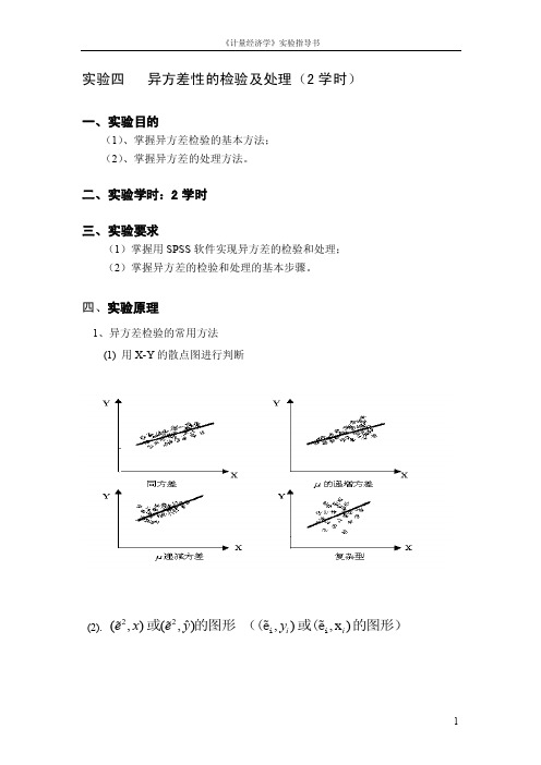
四、实验原理1、异方差检验的常用方法 (1) 用X-Y 的散点图进行判断(2).22ˆ(,)(,)e x e y 或的图形 ,),x )i i y i i ((e 或(e 的图形)(3).等级相关系数法(又称Spearman 检验)是一种应用较广的方法,既可以用于大样本,也可与小样本。
:i u 0原假设H 是等方差的;:i u 0备择假设H 是异方差; 检验的三个步骤 ①ˆt t y y =- i e②|i x i i 将e 取绝对值,并把|e 和按递增或递减次序排序,计算Spearman 系数rs ,其中:21ni i d =∑s 26r =1-n(n -1)|i x i i 其中, n 为样本容量d 为|e 和的等级的差数。
③ 做等级相关系数的显著性检验。
n>8时,(2)t t n =-0当H 成立时,/2(2),t t n α≤-若认为异方差性问题不存在;/2(2),t t n α>-反之,若||i i e x 说明与之间存在系统关系,异方差问题存在。
(4) 帕克(Park)检验帕克检验常用的函数形式:若α在统计上是显著的,表明存在异方差性。
2、异方差检验的处理方法: 加权最小二乘法如果在检验过程中已经知道:222()()()i i i ji u Var u E u f x σσ===则将原模型变形为:121i i p pi iy x x u βββ=⋅⋅++⋅+ 在该模型中:2211)()()()()i i ji u u ji jiVar u Var u f x f x f x σσ===即满足同方差性。
于是可以用OLS 估计其参数,得到关于参数12,,,p βββ 的无偏、有效估计量。
spss最小二乘法求多元线性回归方程

spss最小二乘法求多元线性回归方程
最小二乘法是一种常用的求解多元线性回归方程的方法。
在使用 SPSS 软件求解多元线性回归方程时,可以使用如下步骤:
1.打开 SPSS 软件,在数据窗口中输入需要分析的数据。
2.在 SPSS 的分析菜单中,选择“回归”,然后选择“多元线性回归”。
3.在多元线性回归对话框中,选择“方程”选项卡。
4.在“自变量”框中,选择需要作为自变量的变量。
5.在“因变量”框中,选择需要作为因变量的变量。
6.在“模型”框中,勾选“最小二乘法”复选框。
7.点击“计算”按钮,SPSS 将使用最小二乘法求解多元线性回归方程。
8.在“输出”选项卡中,勾选“方程”复选框,
然后点击“确定”按钮。
SPSS 将计算并输出多元线性回归方程。
在 SPSS 的输出窗口中,可以看到多元线性回归方程的结果。
其中,回归方程的形式为:
Y = b0 + b1X1 + b2X2 + … + bn*Xn
其中,Y 为因变量,X1、X2、…、Xn 为自变量,b0、b1、b2、…、bn 为回归系数。
在输出结果中,还包含了回归系数的估计值、标准误、t 值、p 值等信息。
这些信息可以帮助我们评估回归系数的统计显著性和实际意义。
总的来说,使用 SPSS 软件求解多元线性回归方程时,可以使用最小二乘法的方法,并利用输出结果中的信息评估回归系数的统计显著性和实际意义。
spss课后作业答案
spss课后作业答案SPSS课后作业第⼀章1-1、spss的运⾏⽅式有⼏种?分别是什么?答:SPSS的运⾏⽅式有三种,分别是批处理⽅式、完全窗⼝菜单运⾏⽅式、程序运⾏⽅式。
1-2、SPSS中“DataView”所对应的表格与⼀般的电⼦处理软件有什么区别?答:与⼀般电⼦表格处理软件相⽐,SPSS的“Data View”窗⼝还有以下⼀些特性:(1)⼀个列对应⼀个变量,即每⼀列代表⼀个变量(Variable)或⼀个被观测量的特征;(2)⾏是观测,即每⼀⾏代表⼀个个体、⼀个观测、⼀个样品,在SPSS中称为事件(Case);(3)单元包含值,即每个单元包括⼀个观测中的单个变量值;(4)数据⽂件是⼀张长⽅形的⼆维表。
第⼆章2-1、在SPSS中可以使⽤那些⽅法输⼊数据?答:SPSS中输⼊数据⼀般有以下三种⽅式:(1)通过⼿⼯录⼊数据;(2)可以将其他电⼦表格软件中的数据整列(⾏)的复制,然后粘贴到SPSS中;(3)通过读⼊其他格式⽂件数据的⽅式输⼊数据。
2-2、对于缺失值,如何利⽤SPSS进⾏科学替代?答:选择“Transform”菜单的Replace Missing Values命令,弹出Replace Missing Values 对话框。
先在变量名列中选择1个或多个存在缺失值的变量,使之添加到“New Variable(s)”框中,这时系统⾃动产⽣⽤于替代缺失值的新变量。
最后选择合适的替代⽅式即可。
2-3、在计算数据的加权平均数时,如何对变量进⾏加权?答:选择“Data”菜单中的Weight Cases命令,出现如图2-22所⽰的Weight Cases对话框。
其中, Do not weight cases项表⽰不做加权,这可⽤于取消加权;Weight cases by 项表⽰选择1个变量做加权。
2-4、如何对变量进⾏⾃动赋值?答:变量的⾃动赋值可以将字符型、数字型数值转变成连续的整数,并将结果保存在⼀个新的变量中。
运用SPSS软件对生物统计分析
(运用SPSS软件对生物统计分析)班级学号姓名成绩SPSS方差分析在生物统计的应用摘要:方差分析是生物统计中常采用的一种方法。
如何使用统计分析软件进行方差分析来实现对研究结果的快速和科学的处理,获得正确的结论,是生物学研究中重要的一环。
本文通过实例介绍了如何使用SPSS数据分析工具进行方差分析的方法;实现了数据分析和处理的快捷、准确和直观;与Excel相比,SPSS的统计分析功能更为强大,既有利于提高数据处理效率,又降低了实验成本。
关键词:SPSS 方差分析单因变量多因素方差分析引言:生物学研究离不开统计分析,比较单一或多因素影响下各组别数据之间的差异是生物统计中常用的方法。
如何选择适当的分析软件使差异分析更加快速、便捷,对于研究者来说尤为重要。
常用的分析软件,如:SAS、BMDP、Excel和SPSS等都包含差异分析功能,一般来说所分析数据的种类、软件的功能和使用的便捷性决定了最适合软件的选择。
上述软件中SAS是功能最为强大的统计软件,是熟悉统计学并擅长编程的专业人士的首选。
而SPSS则是非统计学专业人士的首选,其分析结果清晰、直观、易于掌握。
SPSS统计分析软件是20世纪60年代末由美国斯坦福大学的三位研究生共同研制开发的,它借助于数据管理窗口和主窗口的File、Data、Transform等菜单完成,本文通过几个实例介绍了SPSS的数据管理方法以及如何利用SPSS数据分析工具进行方差分析。
l SPSS方差分析的特点方差分析又称变异分析或F检验,用于两个及两个以上样本均数差别的显著性检验。
由于受到各种因素的影响,研究所得的数据呈现波动状,造成波动的原因可分成两类,一类是不可控的随机因素,另一类是研究中施加的对结果形成影响的可控因素。
通过方差分析可评估不同来源的变异对总变异的贡献大小,从而客观地判断可控因素对研究结果影响力的大小旧。
从方差人手的研究方法有助于找到事物的内在规律性。
SPSS适用于社会学、医学、经济学和统计学等多个学科的量化研究。
- 1、下载文档前请自行甄别文档内容的完整性,平台不提供额外的编辑、内容补充、找答案等附加服务。
- 2、"仅部分预览"的文档,不可在线预览部分如存在完整性等问题,可反馈申请退款(可完整预览的文档不适用该条件!)。
- 3、如文档侵犯您的权益,请联系客服反馈,我们会尽快为您处理(人工客服工作时间:9:00-18:30)。
SPSS数据统计分析与实践主讲:周涛副教授北京师范大学资源学院2007-12-4教学网站:/Courses/SPSS第十五章:加权最小二乘法(Weighted Least Squares)本章内容:一、最小二乘法的应用领域z根据需要人为地改变观测量的权重z Remedial Measures for Unequal Error Variances二、SPSS提供的WLS过程z Linear Regression procedure (with weight variable)z Weight Estimation procedure三、相关输出结果的比较z OLS与WLS比较z SPSS提供的两种WLS方法比较加权最小二乘法应用(一)根据需要人为地改变观测量的权重根据需要人为地改变观测量的权重--实例实验中收集的15对数据,每对数据都是将n份样品混合后测得的平均结果,但各对数据的n大小不等,试求出X对Y的线性方程。
数据源:郭祖超,《医用数理统计方法》第三版P249根据需要人为地改变观测量的权重--实例方法一:如果不考虑样品混合量的差异,则该问题是一个非常简单的线性回归问题,可直接拟合回归方程,结果如下:Model Summary b.987a.975.973.11330Model1R R SquareAdjustedR SquareStd. Error ofthe Estimate Predictors: (Constant), xa.Dependent Variable: yb.Coefficients a7.454.17343.143.000-.015.001-.987-22.468.000 (Constant)xModel1B Std. ErrorUnstandardizedCoefficientsBetaStandardizedCoefficientst Sig.Dependent Variable: ya.Y = 7.45 –0.015 * X (R2=0.98)根据需要人为地改变观测量的权重--实例方法二:由于每对测量数据都是将n份样品混合后测得结果,显然混合的样品越多,测得的结果越稳定,即变异越小。
如果直接拟合方程,则是将所有测量值均一视同仁,1份样品的测量结果与15份样品混合后的测量结果等价对待,这显然不太合理。
为此可以考虑在分析中将样品数n作为权重变量,n 值越大的观测量在计算中给予的权重越高,对方程的影响越大,即按照加权最小二乘法来拟合回归方程。
根据需要人为地改变观测量的权重--实例z SPSS操作步骤:z AnalyzeÆRegressionÆLinearz Dependent: Yz Independent: Xz WLS Weight: nWLS WeightWLS: Weighted Least SquaresWLS 输出结果Model Summary b,c.982a.965.962.29365Model 1RR SquareAdjusted R SquareStd. Error of the EstimatePredictors: (Constant), x a. Dependent Variable: yb. Weighted Least Squares Regression - Weighted by nc. Y = 7.19 –0.014 * X (R 2=0.97)Coefficients a,b7.190.18838.316.000-.014.001-.982-18.816.000(Constant)xModel 1B Std. Error Unstandardized Coefficients BetaStandardizedCoefficientstSig.Dependent Variable: ya. Weighted Least Squares Regression - Weighted by nb.WLS 与OLS 输出结果比较1.在OLS中,测定系数为0.975, 而在WLS中测定系数降低为0.965。
2.由于测定系数是按照普通最小二乘法进行计算,因此加权后的方程测定系数必然小于普通最小二乘法,即此时不能使用测定系数来判断模型的优劣。
WLS 与OLS 输出结果比较3. 通过绘制OLS和WLS的回归直线加以比较,如下图所示,WLS更靠近中部那些混合样品数据n较大的测量值,而对两端n较小的测量值则比OLS回归直线更远一些,显然这些测量值在计算时对方程的影响程度是不同的。
实现WLS的另一种方法z事实上,如果使用SPSS的Weight Case过程,将n指定为频数变量,然后进行普通的线性回归,得到的分析结果与上述加权最小二乘法完全相同。
z操作过程如下所示:实现WLS的另一种方法步骤:(1)调用Weight Case过程DataÆWeight Cases…)(2)调用线性回归过程(采用OLS)实现WLS 的另一种方法—输出结果Model Summary b,c.982a.965.962.29365Model 1RR SquareAdjusted R SquareStd. Error of the EstimatePredictors: (Constant), x a. Dependent Variable: yb. Weighted Least Squares Regression - Weighted by nc. Y = 7.19 –0.014 * X (R 2=0.97)Coefficients a,b7.190.18838.316.000-.014.001-.982-18.816.000(Constant)xModel 1B Std. Error Unstandardized Coefficients BetaStandardizedCoefficientstSig.Dependent Variable: ya. Weighted Least Squares Regression - Weighted by nb.加权最小二乘法应用(二)Unequal Error Variances Remedial Measures ----Weighted Least SquaresVariation of Errors Around the Regression LineX1X 2XYf(e)1. y values are normally distributedaround the regression line.2. For each x value, the “spread”orvariance around the regression line isthe same.Regression LineEqual Error Variancesip i p i i i X X X Y εββββ+++++=−−1,122110K 110,,−p βββK are parameters1,21,,,−p i i i X X X K are known constantsi εare independent ),0(2σN ni ,,1L =Equal error variance(1)111)(××−××′′=p p p pp p YX X X b (2)ip i p i i i X X X Y εββββ+++++=−−1,122110K 110,,−p βββK are parameters1,21,,,−p i i i X X X K are known constantsi εare independent ),0(2iN σni ,,1L =Unequal error variance⎥⎥⎥⎥⎥⎦⎤⎢⎢⎢⎢⎢⎣⎡=×222212000000}{n n n σσσεσK MM M K K (3)z The estimation of the regression coefficients in generalized model (3)could be done by using the estimators in (2)for regression model (1)with equal error variances. These estimators are still unbiased and consistent for model (3),but they no longer have minimum variance.z To obtain unbiased estimators with minimum variance, we must take into account that the different Y observations for the n cases no longer have the same reliability.z Observations with small variances provide more reliable information about the regression function than those with large variances.Error Variances KnownError Variances KnownWe first consider the estimation of the regressionfunction coefficients when the error varianceare known . This case is usually unrealistic, but it provides guidance as to how to proceed when the error variances are not know.2i σError Variances KnownWhen the error variances are known, we can usethe method of maximum likelihood to obtainestimators of the regression coefficients in (3).2i σ])(21exp[)2(1)(21,1110212/12−−=−−−−−=∏p i p i i i n i i X X Y L βββσπσK βwhere βdenotes the vector of the regression coefficients. We define the reciprocal of the variance as the weight w i :2i σ21i i w σ=(4)(5)⎥⎦⎤⎢⎣⎡−−−−−⎥⎦⎤⎢⎣⎡=−−=∑∏21,1110112/1)(21exp )2()(p i p i i n i n i i X X Y w w L βββπK β(6)Error Variances Known⎥⎦⎤⎢⎣⎡−−−−−⎥⎦⎤⎢⎣⎡=−−=∑∏21,1110112/1)(21exp )2()(p i p i i n i ni i X X Y w w L βββπK β(6)We find the maximum likelihood estimators of theregression coefficients by maximizing L(β)in formula (6)with respect to .110,,,−p βββK Since the error variances and hence the weightsare assumed to be known, maximizing L(β)with respect to the regression coefficients is equivalent to minimizing the exponential term :2i σi w 21,11101)(−−=−−−−=∑p i p i i n i i w X X Y w Q βββK (7): weight least squares criterionw QError Variances Known•Since the weight is inversely related to the variance , it reflects the amount of information contained in the observation Yi.•Thus, an observation Yi that has a large variance receivesless weight than another observation that has a small variance.•Intuitively, this is reasonable. The more precise is Yi (i.e.,the smaller is ), the more information Yi provides aboutE{Yi }and therefore the more weight it should receive infitting the regression function.2i σiw2iσLet the matrix W be a diagonal matrix containing the weight :i w ⎥⎥⎥⎥⎦⎤⎢⎢⎢⎢⎣⎡=×n n n w w w W K M M M K K 00000021The normal equations can then be expressed as follows:WYX b WX X w′=′)(and the weighted least squares and maximum likelihood estimators of the regression coefficients are:WYX WX X b w ′′=−1)(where b w is the vector of the estimated regressioncoefficients obtained by weighted least squares.(8)(9)(10)•The weighted least squares and maximum likelihood estimators of the regression coefficients in formula (10) are unbiased, consistent, and have minimum variance among unbiased linear estimator.•Thus, when the weights are known, bw generally exhibitsless variability than the ordinary least squares estimator b.Error Variances UnknownError Variances Unknownz If the variances of errors were known, the use of weighted least squares with weights wi would be straightforward.z Unfortunately, one rarely has knowledge of the variances of errors. We are then forced to use estimates of the variances.Estimation of Variance Function z The magnitudes of error variances often vary in a regular fashion with one or severalpredictor variables Xk or with the meanresponse E{Yi}.X ez Such a relationship between and one or several predictor can be estimated because the squared residual obtained from an ordinary least squares regression fit is an estimate of , provided that theregression function is appropriate.X e2i σ2i e 2i σ}{22ii E εσ=Some possible variance functions:1.A residual plot against X 1exhibits a megaphone shape . Regress the absolute residuals against X 1.2.A residual plot against exhibits a megaphone shape. Regress the absolute residuals against .3.A plot of squared residuals against X 3exhibits an upward tendency. Regress the squared residuals against X 3.4. A plot of the residuals against X 2suggests that the varianceincreases rapidly with increases in X 2up to a point and then increases more slowly. Regree the absolute residualsagainst X 2and .Y ˆY ˆ22XSummary of the WLS estimation process1.Fit the regression model by unweighted leastsquares and analyze the residuals.2.Estimate the variance function by regression eitherthe squared residuals or the absolute residuals onthe appropriate predictor(s).e the fitted values from the estimated varianceto obtain the weights w.i4.Estimate the regression coefficients using theseweights.SPSS Example of WLSExamplez A health researcher, interested in studying the relationship between diastolic blood pressure(舒张压) and age among healthy adult women 20 to 60 years old, collected data on 54 subjects.Step 1: Preliminary analysesBlood_Pressure= 56.157 + 0.58003 * Age Nonconstant errorvarianceStep 2: Estimating the variance functionThe plot of the absolute residuals against X suggests that a linearrelation between the error standard deviation and X maybe reasonable.Age s×+=198.0549.1ˆdenotes the estimated expected standard deviationsˆTo obtain the weights w i , the analyst obtained the fitted values from the standard deviation function in (11). For case 1 (X 1=27)(11)801.327198.0549.1ˆ1=×+=s0692.0)801.3(1)ˆ(12211===s wStep 2: Estimating the variance functionX i Yiei|ei|isˆi w21)ˆ(1swi=Step 3: Weighted Least SquaresX Y596.0566.55ˆ+=Coefficients a,b55.566 2.52122.042.000.596.079.7227.526.000(Constant)AgeModel 1B Std. Error Unstandardized Coefficients BetaStandardizedCoefficientstSig.Dependent Variable: Blood_Pressurea. Weighted Least Squares Regression - Weighted by wib. (12)Step 4: Comparison of WLS and OLSCoefficients a56.157 3.99414.061.000.580.097.6395.983.000(Constant)AgeModel 1B Std. Error Unstandardized Coefficients BetaStandardizedCoefficientstSig.Dependent Variable: Blood_Pressurea. Coefficients a,b55.566 2.52122.042.000.596.079.7227.526.000(Constant)AgeModel 1B Std. Error Unstandardized Coefficients BetaStandardizedCoefficientstSig.Dependent Variable: Blood_Pressurea. Weighted Least Squares Regression - Weighted by wib. OLSWLSb w generally exhibits less variability than the ordinary least squares estimator bIt is interesting to note that this Std. is somewhat smaller than the Std.of the estimate obtained by OLS. The reduction of about 18% is the result of the recognition of unequal error variances when using WLS.Step 4: Comparison of WLS and OLSCoefficients a56.157 3.99414.061.000.580.097.6395.983.000(Constant)AgeModel 1B Std. Error Unstandardized Coefficients BetaStandardizedCoefficientstSig.Dependent Variable: Blood_Pressurea. Coefficients a,b55.566 2.52122.042.000.596.079.7227.526.000(Constant)AgeModel 1B Std. Error Unstandardized Coefficients BetaStandardizedCoefficientstSig.Dependent Variable: Blood_Pressurea. Weighted Least Squares Regression - Weighted by wib. OLSWLSSince the regression coefficients changed only a little , the analyst concluded that there was no need to reestimate the standard deviation function and the weights based on the residuals for the weighted regression in formula (12).Step 4: Comparison of WLS and OLS If the estimated coefficients differ substantially from the estimated regression coefficients obtained by OLS, it is usually advisable to iterate the WLS process by using the residuals from the WLS fit to reestimate the variance or Std. Function and then obtain revised weights. This iteration process is often called iteratively reweighted least squares.SPSS Weight Estimation procedureSPSS Weight Estimation procedurez尽管采用SPSS Linear Regression过程(人为确定WLS Weight变量)可以用于WLS,但两个因素使得使用该过程比较麻烦:1.有时WLS Weight变量值不容易确定。