ADAMS接触力汇总
adams中接触力参数

在ADAMS(Automatic Dynamic Analysis of Mechanical Systems)中,接触力参数的设置对于模拟接触行为和计算接触力至关重要。
以下是一些常见的接触力参数:1. 接触类型:二维(2D)接触:适用于平面几何形状之间的接触,如圆弧、曲线和点。
三维(3D)接触:适用于实体之间的接触,如球、圆柱、封闭的shell、拉伸体和旋转体。
2. 接触算法:基于回归的接触算法(Restitution-base contact):通过惩罚参数与回归系数计算接触力,考虑能量损失和恢复系数。
基于碰撞函数的接触算法(IMPACT-Function-based contact):使用ADAMS函数库中的IMPACT函数来计算接触力。
3. 接触参数:刚度(Stiffness):描述接触面抵抗变形的能力,单位通常为N/m或N/mm。
力指数(Force Exponent):影响接触力随位移变化的曲线形状,通常取值在1.1~1.5之间。
最大阻尼系数(Damping):控制接触过程中能量耗散的速度,单位通常为N·s/m。
穿透深度(Penetration Depth):允许接触体在没有产生接触力的情况下相互穿透的最大距离,单位通常为m。
静摩擦系数(Static Friction Coefficient):描述接触面在相对静止时阻止滑动的阻力。
动摩擦系数(Kinetic Friction Coefficient):描述接触面在相对运动时阻止滑动的阻力。
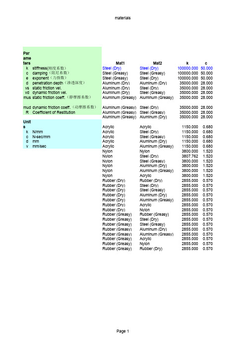
4. 材料相关参数:材料stiffness 和damping:这些参数取决于具体材料的物理特性,例如钢(Steel)在干燥或润滑条件下的刚度和阻尼系数。
在设置这些参数时,需要根据实际的机械系统和材料特性进行调整,以确保模拟结果的准确性和可靠性。
虚拟样机详述Adams中接触的定义
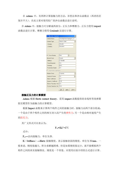
在Adams中,有两种计算接触力的方法:补偿法和冲击函数法(两者的差别并不大)。
在此主要对使用较广的冲击函数法进行说明。
在Adams中,接触力可分解成两部分:正压力和摩擦力。
正压力使用impact 函数法进行计算,摩擦力使用Coulomb法进行计算。
接触正压力的计算模型Adams根据Hertz contact theory,采用impact函数提供的非线性等效弹簧阻尼模型作为接触力的计算模型。
根据Impact函数来计算两个构件之间的接触力时,接触力由两个部分组成:一个是由于两个构件之间的相互切入而产生的弹性力;另一个是由相对速度产生的阻尼力。
其广义形式可以表示为:F ni=Kδi e+CV i式中:F ni—法向接触力,单位为N。
K(Stiffness)—Hertz接触刚度,表示接触表面的刚度,单位为N/mm。
一般来说,刚度值越大,积分求解越困难,但是如果刚度值过小,就不能模拟两个构件之间的真实接触情况。
刚度是一个常值,应使用后面介绍的公式进行计算。
δi(Penetration Depth)—接触点的法向穿透深度,单位为mm。
注意:接触定义界面中输入的是阻尼达到最大值时的穿透深度(由碰撞动力学模型可知,两物体接触后,阻尼很快就达到最大值,且在接触过程中保持不变,因此,此时输入的穿透深度的取值应该越小越好。
同时考虑到ADAMS中的数值收敛性,一般可采用ADAMS中推荐的取值0.01 mm),并不是最大穿透深度(阻尼达到最大值后,构件之间的相互切入还可以继续)。
当接触点的法向穿透深度小于其临界值(接触定义界面中的输入值)时,阻尼系数是穿透深度的三次函数,当大于等于临界值时,阻尼值也到达其最大值,如下图所示。
e(Force Exponent)—力的指数,刚度项的贡献因子。
对于刚度比较大的接触,e>1,否则e<1。
对于金属常用1.3~1.5,对于橡胶可取2甚至3。
一般用1.5。
C(Damping)—阻尼系数,单位为N*sec/mm。
adams各种材料接触参数设置
Page 1
terials
e
d
vs vd mus mud R
1.5 0.1 0.1
10 0.3 0.25 0.15
1.5 0.1 0.1
10 0.08 0.05 0.15
1.5 0.1 0.1
10 0.08 0.05 0.15
1.5 0.1 0.1
10 0.25 0.2 0.20
1.5 0.1 0.1
2 0.1 0.1 2 0.1 0.1 2 0.1 0.1 2 0.1 0.1 2 0.1 0.1 2 0.1 0.1 2 0.1 0.1 2 0.1 0.1 2 0.1 0.1 2 0.1 0.1 2 0.1 0.1 1.1 0.1 0.1 1.1 0.1 0.1 1.1 0.1 0.1 1.1 0.1 0.1 1.1 0.1 0.1 1.1 0.1 0.1 1.1 0.1 0.1 1.1 0.1 0.1 1.1 0.1 0.1 1.1 0.1 0.1 1.1 0.1 0.1 1.1 0.1 0.1 1.1 0.1 0.1 1.1 0.1 0.1 1.1 0.1 0.1
materials
Par
ame
ters k stiffness(刚度系数) c damping(阻尼系数) e exponent(力指数) d penetration depth(渗透深度)
vs static friction vel.
vd dynamic friction vel. mus static friction coeff.(静摩擦系数)
0.680 0.680 0.680 0.680 0.680 1.520 1.520 1.520 1.520 1.520 1.520 0.570 0.570 0.570 0.570 0.570 0.570 0.570 0.570 0.570 0.570 0.570 0.570 0.570 0.570 0.570
虚拟样机详述Adams中接触的定义
在Adams中,有两种计算接触力的方法:补偿法和冲击函数法(两者的差别并不大)。
在此主要对使用较广的冲击函数法进行说明。
在Adams中,接触力可分解成两部分:正压力和摩擦力。
正压力使用impact 函数法进行计算,摩擦力使用Coulomb法进行计算。
接触正压力的计算模型Adams根据Hertz contact theory,采用impact函数提供的非线性等效弹簧阻尼模型作为接触力的计算模型。
根据Impact函数来计算两个构件之间的接触力时,接触力由两个部分组成:一个是由于两个构件之间的相互切入而产生的弹性力;另一个是由相对速度产生的阻尼力。
其广义形式可以表示为:F ni=Kδi e+CV i式中:F ni—法向接触力,单位为N。
K(Stiffness)—Hertz接触刚度,表示接触表面的刚度,单位为N/mm。
一般来说,刚度值越大,积分求解越困难,但是如果刚度值过小,就不能模拟两个构件之间的真实接触情况。
刚度是一个常值,应使用后面介绍的公式进行计算。
δi(Penetration Depth)—接触点的法向穿透深度,单位为mm。
注意:接触定义界面中输入的是阻尼达到最大值时的穿透深度(由碰撞动力学模型可知,两物体接触后,阻尼很快就达到最大值,且在接触过程中保持不变,因此,此时输入的穿透深度的取值应该越小越好。
同时考虑到ADAMS中的数值收敛性,一般可采用ADAMS中推荐的取值0.01 mm),并不是最大穿透深度(阻尼达到最大值后,构件之间的相互切入还可以继续)。
当接触点的法向穿透深度小于其临界值(接触定义界面中的输入值)时,阻尼系数是穿透深度的三次函数,当大于等于临界值时,阻尼值也到达其最大值,如下图所示。
e(Force Exponent)—力的指数,刚度项的贡献因子。
对于刚度比较大的接触,e>1,否则e<1。
对于金属常用1.3~1.5,对于橡胶可取2甚至3。
一般用1.5。
C(Damping)—阻尼系数,单位为N*sec/mm。
ADAMS接触与摩擦力简介
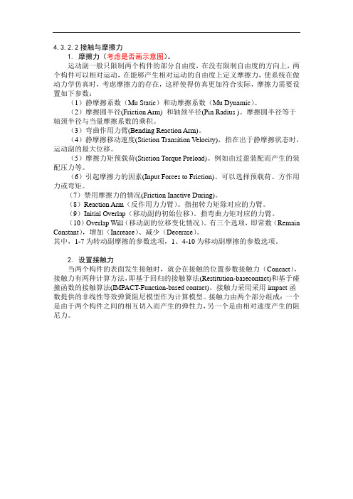
4.3.2.2接触与摩擦力1. 摩擦力(考虑是否画示意图)。
运动副一般只限制两个构件的部分自由度,在没有限制自由度的方向上,两个构件可以相对运动,在能够产生相对运动的自由度上定义摩擦力,使系统在做动力学仿真时,考虑摩擦力的存在,这样使得仿真更加符合实际,摩擦力需要设置如下参数:(1)静摩擦系数(Mu Static)和动摩擦系数(Mu Dynamic)。
(2)摩擦圆半径(Friction Arm) 和轴颈半径(Pin Radius )。
摩擦圆半径等于轴颈半径与当量摩擦系数的乘积。
(3)弯曲作用力臂(Bending Reaction Arm)。
(4)静摩擦移动速度(Stiction Transition Velocity),指在出于静摩擦状态时,运动副的最大位移。
(5)摩擦力矩预载荷(Stiction Torque Preload)。
例如由过盈装配而产生的装配压力等。
(6)引起摩擦力的因素(Input Forces to Friction)。
可以选择预载荷、方作用力或弯矩。
(7)禁用摩擦力的情况(Friction Inactive During)。
(8)Reaction Arm(反作用力力臂)。
指扭转力矩除对应的力臂。
(9)Initial Overlap(移动副的初始位移)。
指弯曲力矩对应的力臂。
(10)Overlap Will(移动副的位移变化情况)。
有三个选项,即常数(Remain Constant),增加(Increace)、减少(Decerase)。
其中,1-7为转动副摩擦的参数选项,1、4-10为移动副摩擦的参数选项。
2. 设置接触力当两个构件的表面发生接触时,就会在接触的位置参数接触力(Concact),接触力有两种计算方法,即基于回归的接触算法(Restitution-basecontact)和基于碰撞函数的接触算法(IMPACT-Function-based contact)。
接触力采用采用impact函数提供的非线性等效弹簧阻尼模型作为计算模型。
adams中接触力参数
adams中接触力参数在力学中,接触力是指两个物体之间的相互作用力。
对于光滑表面,可以通过分析各种因素来确定接触力的参数。
总的来说,接触力参数可以分为以下几个方面:表面形貌、表面粗糙度、接触面积、弹性模量、材料硬度等。
首先,表面形貌对接触力参数的影响很大。
例如,对于两个接触表面,如果其中一个表面具有凸起的形状,而另一个表面是平坦的,那么接触力将主要由凸起部分上的接触区域决定。
这是因为凸起部分有更高的位置,会承受更高的压力。
因此,凸起部分的形状和尺寸将直接影响接触力的大小。
其次,表面粗糙度也会影响接触力参数。
粗糙表面上存在着更多的微小凸起和凹陷,使得接触面积变大,从而增加了接触力。
此外,粗糙表面还会增加摩擦力,使物体之间更难相对移动。
因此,在分析接触力参数时,需要考虑表面的粗糙度,并根据具体情况调整相关参数。
接下来是接触面积对接触力参数的影响。
接触面积是指两个物体之间实际接触的表面积。
通常,接触面积越大,接触力就越大。
这是因为接触力与单位面积上的压力成正比。
例如,当一个球形物体通过液体或柔软材料时,只有一个点和液体或材料接触,因此接触面积很小,接触力也相对较小。
此外,弹性模量也是影响接触力参数的因素之一。
弹性模量是物体对应力或应变的响应能力。
对于具有不同弹性模量的物体,其接触力也会有所不同。
当两个物体接触时,弹性模量较大的物体更难被压缩和变形,因此会产生更大的接触力。
最后,材料硬度也会对接触力参数产生影响。
材料硬度是材料抵抗局部形变和划痕的能力。
当硬度较大的物体接触时,它们更难被压缩和变形,因此会产生更大的接触力。
综上所述,接触力参数的确定涉及到多个因素,包括表面形貌、表面粗糙度、接触面积、弹性模量和材料硬度等。
这些参数的具体数值需要通过实验或模拟分析获得,从而更好地确定接触力。
在工程设计和材料选择中,准确地了解和控制接触力参数对于确保结构安全和材料性能至关重要。
adams中的接触力算法

Contacts•Overview•Contact Force Algorithms•Supported Geometry in Contacts•Creating/Modifying Contact Forces•Simulation Results of Contact Forces•Learning More about the Contact Detection Algorithm•Contact Friction Force Calculation•Material Contact Properties TableOverviewUsing contacts, you can go beyond just modeling how parts meet at points and model how solid bodies react when they come in contact with one another when the model is in motion.For more on the theory behind contact forces, see the CONTACT statement in the Adams/Solver online help.See Solver Settings - Contacts dialog box help.About Contact ForcesContacts allow you to model how free-moving bodies interact with one another when they collide during a simulation.Contacts are grouped into two categories:•Two-dimensional contacts, which include the interaction between planar geometric elements (for example, circle, curve, and point)•Three-dimensional contacts, which include the interaction between solid geometry (for example, spheres, cylinders, enclosed shells, extrusions, and revolutions).You currently cannot model contact between a two-dimensional and a three-dimensional geometry, except for sphere-to-plane contact.For more on the theory behind contact forces, see the CONTACT statement in the Adams/Solver online help.Click here to see an Example of Using Contact Forces.Contact Force AlgorithmsContact forces use two distinct normal force algorithms:•Restitution-based contactAdams/View Contacts 288•IMPACT-Function-Based ContactYou can also create your own contact force model by entering parameters to a User-written subroutine .Supported Geometry in ContactsTwo-Dimensional ContactsAdams/View supports two-dimensional contact between the following geometry:•Arc•Circle•Polylines•Splines•Point•PlaneFor flexible bodies, only point-to-plane and point-to-curve contacts are supported, where the point is on the flexible body. Adams/Solver (C++) can treat multiple points per CONTACT statement. Adams/Solver (FORTRAN) can only treat one point per CONTACT statement.Three-Dimensional ContactsAdams/View supports three-dimensional contact between the following solid geometry:•Sphere•Cylinder•Frustum•Box•Link•TorusNote:Contact defined between planar geometry (for example, circle to curve) must beconstrained to lie in the same plane. You usually accomplish this using planar joints or anequivalent set of Constraint s that enforce the planarity.Failure to enforce planarity will result in a run-time error when the bodies go out of planeduring a Simulation .Note:You cannot have contacts between a point and another point and a plane and another plane.289Contacts•Extrusion•Revolution•Constructive, solid geometry (geometry combined from several geometries)•Generic three-dimensional Parasolid geometry, including extrusion and revolution•Shell (enclosed-volume only)You can also create a contact between a three-dimensional elliposoid and a plane (sphere only).In case of Adams/Solver C++, you can create three-dimensional contacts between flexible bodies as wellas between a flexible body and a Solid geometry. When a three-dimensional contact is created betweena flexible body and a solid geometry, it is mandatory that the rigid body is always the J geometry.Adams/View also supports nonsolid, three-dimensional geometries, such as shells. Adams/View allows you to select the free edges of shell elements. You can create contacts between flexible body edges aswell as between flexible body edge and a plane or a curve.Creating/Modifying Contact ForcesTo create or modify a contact force:1.From the Force tool stack or palette, select the Contact Force tool .The Create/Modify Contact dialog box appears.2.Enter values in the dialog box as explained in the table below, and then select OK.Tip:You can change the direction of the force on some geometry (for example, circle, curve,plane, and sphere) by selecting the Change Direction tool .Adams/ViewContacts290Define type and geometry To define the geometry/flexible body that comes into contact:1.Set Type to the type of geometry to come into contact. In case offlexible bodies, you must either select the Flex Body To Flex Bodyor Flex Body to Solid options. Flexible bodies can participate inthe contact only for Adams/Solver C++. In case of flex edgecontacts, select Flex Edge To Flex Edge or Flex Edge To Curve orFlex Edge To Plane.The text boxes change depending on the type of contact force youselected.2.In the text boxes, enter the name of the geometry or flexible bodyobjects. For solids and curves, you can enter more than onegeometry, but the geometry must belong to the same part. You canselect the objects from the screen or Database Navigator or type itdirectly in the text box. If you type the geometry object namedirectly in the text box, you must press Enter to register the value.In case of "Flex Body to Solid" type of contacts, the rigid bodyshould always be the J geometry. Similarly in case of Flex Edge toCurve or Plane type of contacts, Curve or Plane should always beJ geometries.Tips on Entering Object Names in Text Boxes.If you want to change the direction of the force, in the Directionpull-down menu, select the geometry on which you want to changethe force, and then select the Change Direction tool . Thisis disabled in case of "Flex Body to Flex Body" and "Flex Body toSolid" contacts but is available in all the Flex Edge contacts.Turn on the force display for both normal and friction forces and set its color Select Force Display, and then from the option menu, select a color for the force display.Note:If you are using an External Adams/Solver, you must set the output files to XML to view the force display. See SolverSettings - Output dialog box helpRefine the normal force between two sets of rigid geometries that are in contact Select Augmented Lagrangian.When you select Augmented Lagrangian, Adams/View uses iterative refinement to ensure that penetration between the geometries is minimal. It also ensures that the normal force magnitude is relatively insensitive to the penalty or stiffness used to model the local material compliance effects.Note:Augmented Lagrangian is only available when defining a Restitution-based contact.291 ContactsDefine a restitution-based contact To define the normal force as restitution-based:1.Set Normal Force to Restitution.2.Enter a penalty value to define the local stiffness propertiesbetween the contacting material.A large penalty value ensures that the penetration of one geometryinto another will be small. Large values, however, will causenumerical integration difficulties. A value of 1E6 is appropriatefor systems modeled in Kg-mm-sec. For more information on how to specify this value, see the Extended Definition for theCONTACT statement in the Adams/Solver online help.3.Enter the coefficient of restitution, which models the energy lossduring contact.4.A value of zero specifies a perfectly plastic contact between thetwo colliding bodies.5.A value of one specifies a perfectly elastic contact. There is noenergy loss.The coefficient of restitution is a function of the two materials that are coming into contact. For information on material types versus commonly used values of the coefficient of restitution, see the table for the CONTACT statement in the Adams/Solver online help. Restitution based contacts is not available when flexible bodies are participating in the contact.Adams/ViewContacts292Define an impact contact To define the normal force as based on an impact using the IMPACTfunction:1.Set Normal Force to Impact.2.Enter values for the following:•Stiffness - Specifies a material stiffness that is to be used tocalculate the normal force for the impact model.In general, the higher the stiffness, the more rigid or hard thebodies in contact are.Note:When changing the length units in Adams/View, stiffnesses incontacts are scaled by (length conversion factor**exponent).When changing the force unit, stiffness is only scaled by theforce conversion factor.•Force Exponent - Adams/Solver models normal force as anonlinear springdamper. If the damping penetration, above, isthe instantaneous penetration between the contactinggeometry, Adams/Solver calculates the contribution of thematerial stiffness to the instantaneous normal forces as:STIFFNESS * (PENALTY)**EXPONENTFor more information, see the IMPACT function in theAdams/Solver online help.•Damping - Enter a value to define the damping properties ofthe contacting material. A good rule of thumb is that thedamping coefficient is about one percent of the stiffnesscoefficient.•Penetration Depth - Enter a value to define the penetration atwhich Adams/Solver turns on full damping. Adams/Solveruses a cubic STEP function to increase the damping coefficientfrom zero, at zero penetration, to full damping when thepenetration reaches the damping penetration. A reasonablevalue for this parameter is 0.01 mm. For more information,refer to the IMPACT function in the Adams/Solver online help.Define your own contact model 1.Set Normal Force to User Defined.2.Enter parameters to the user-defined subroutine. You can alsospecify an alternative library and name for the user subroutine in the Routine text box. Learn about ROUTINE Argument.293ContactsModel the friction effectsat the contact locations using the Coulombfriction modelNote:The friction model models dynamic friction but not stiction.For more on friction in contacts, see Contact Friction Force Calculation . In addition, read the information for the CONTACT statement in the Adams/Solver online help.1.Set Friction Force to Coulomb .2.Set Coulomb Friction to On , Off , or Dynamics Only to define whether friction effects are to be included.3.In the Static Coefficient text box, specify the coefficient of friction at a contact point when the slip velocity is smaller than the value for Static Transition Vel . For information on material types versus commonly used values of the coefficient of static friction,see Material Contact Properties Table .Excessively large values of Static Coefficient can causeintegration difficulties.Range: Static Coefficient 04.In the Dynamic Coefficient text box, specify the coefficient offriction at a contact point when the slip velocity is larger than thevalue for Friction Transition Vel. For information on materialtypes versus commonly used values of the coefficient of thedynamic coefficient of friction, see Material Contact PropertiesTable .Excessively large values of Dynamic Coefficient can causeintegration difficulties.Range: 0 Dynamic Coefficient Static Coefficient5.In the Static Transition Vel . text box, enter the static transitionvelocity. Learn more about this value .6.In the Friction Transition Vel . text box, enter the frictiontransition velocity.Adams/Solver gradually transitions the coefficient of friction fromthe value for Static Coefficent to the value for DynamicCoefficient as the slip velocity at the contact point increases.When the slip velocity is equal to the value specified for FrictionTransition Vel., the effective coefficient of friction is set toDynamic Coefficient.Note:Small values for this option cause the integrator difficulties. You should specify this value as:Friction Transition Vel. 5* ERRORwhere ERROR is the integration error used for the solution. Itsdefault value is 1E-3.Range: Friction Transition Vel. Static Transition Vel. > 0Adams/View Contacts 294Simulation Results of Contact ForcesWhen you run a simulation, Adams/View automatically calculates specific attributes of contact forces. The results appear in Adams/PostProcessor in plotting mode for objects.For contact force:•element_force•element_torqueFor tracks:•Double-click a track to view:•I_Point•I_Normal_Force•I_Friction_Force•I_Normal_Unit_Vector•I_Friction_Unit_Vector•J_Point•J_Normal_Force•J_Friction_ForceModel the friction effects at the contact locationsusing your own model 1.Set Friction Force to User Defined .2.Enter parameters to a user-defined subroutine, CNFSUB , and enterthe name of the routine.3.In the Static Transition Vel . text box, enter the static transitionvelocity.Adams/Solver gradually transitions the coefficient of friction fromthe value in Dynamic Coefficient to the value in Static Coefficentas the slip velocity at the contact point decreases. When the slipvelocity is equal to the value you specify for Static Transition Vel.,the effective coefficient of friction is set to the value in StaticCoefficient.Range: 0 < Static Transition Vel. Friction Transition VelNote: A small value for Static Transition Vel. causes numerical integrator difficulties. A general rule for specifying this value is:Static Transition Vel. ERRORwhere ERROR is the accuracy requested of the integrator. Itsdefault value is 1E-3. See Solver Settings - Dynamic .295Contacts•J_Normal_Unit_Vector•J_Friction_Unit_Vector•Slip_Deformation•Slip_Velocity•PenetrationLearning More about the Contact Detection AlgorithmTo greatly simplify the contact detection algorithm, Adams/Solver assumes that the volume of intersection between two solids will be much, much less than the volume of either solid. This means that,for example for a sphere in a V-groove, the Adams/Solver algorithm breaks down when the two contact volumes merge into one. This assumption is not as drastic as it may first appear. The reason is that most users are interested in contact between rigid bodies (that is, bodies that do not undergo a large deformation). Also, rigid bodies generally do not penetrate very far into one another. Note that we do not recommend that you use the contact detection algorithm in the modeling of very soft bodies.After contact occurs between two solids, Adams/Solver computes the volumes of intersection. There maybe only one volume of intersection, or there may be multiple volumes of intersection (this would correspond to multiple locations of contact). In this discussion, we assume that there is only a single volume of intersection. The algorithm is the same for every intersection volume.Once there is contact, Adams/Solver finds the centroid of the intersection volume. This is the same as the center of mass of the intersection volume (assuming the intersection volume has uniform density).Next, Adams/Solver finds the closest point on each solid to the centroid. The distance between these two points is the penetration depth.Adams/Solver then puts this distance into the formula:F = K*(distance)nwhere:•K - material stiffness•n - exponent• F - forceto determine the contact force due to the material stiffness (there can also be damping and friction forcesin the contact).For example, if you apply this algorithm to a sphere on a plate, the intersection volume is some type of spherical shape with a flat side. The centroid of this volume can be computed (this is where most of the time is spent in the algorithm). It will be below the plate and inside the sphere. The nearest point on the plate (to the centroid) and the nearest point on the sphere (to the centroid) can also be computed. In this case, the line between them will pass through the center of the sphere (this will also be the direction in which the contact force acts).Adams/View296ContactsAgain, the algorithm can handle the case of a sphere in a V-groove. There will be two volumes ofintersection and two separate forces will be applied to sphere and to the V-groove (equal and oppositeforces).Contact Friction Force CalculationAdams/Solver uses a relatively simple velocity-based friction model for contacts. Specifying thefrictional behavior is optional. The figure below shows how the coefficient of friction varies with slipvelocity.Coefficient of Friction Varying with Slip VelocityContacts In this simple model:Material Contact Properties TableThe table below shows material types and their commonly used values for the dynamic coefficient of friction and restitution.Material 1:Material 2:Mu static:Mu dynamic:Restitution Coefficient: Dry steel Dry steel0.700.570.80Greasy steel Dry steel0.230.160.90Greasy steel Greasy steel0.230.160.90Dry aluminium Dry steel0.700.500.85Dry aluminium Greasy steel0.230.160.85 Dry aluminium Dry aluminium0.700.500.85 Greasy aluminium Dry steel0.300.200.85 Greasy aluminium Greasy steel0.230.160.85 Greasy aluminium Dry aluminium0.300.200.85 Greasy aluminium Greasy aluminium0.300.200.85 Acrylic Dry steel0.200.150.70 Acrylic Greasy steel0.200.150.70 Acrylic Dry aluminium0.200.150.70 Acrylic Greasy aluminium0.200.150.70 Acrylic Acrylic0.200.150.70 Nylon Dry steel0.100.060.70 Nylon Greasy steel0.100.060.70 Nylon Dry aluminium0.100.060.70 Nylon Greasy aluminium0.100.060.70 Nylon Acrylic0.100.060.65 Nylon Nylon0.100.060.70 Dry rubber Dry Steel0.800.760.95 Dry rubber Greasy steel0.800.760.95 Dry rubber Dry aluminium0.800.760.95 Dry rubber Greasy aluminium0.800.760.95 Dry rubber Acrylic0.800.760.95 Dry rubber Nylon0.800.760.95 Dry rubber Dry rubber0.800.760.95 Greasy rubber Dry steel0.630.560.95 Greasy rubber Greasy steel0.630.560.95 Greasy rubber Dry aluminium0.630.560.95 Greasy rubber Greasy aluminium0.630.560.95 Greasy rubber Acrylic0.630.560.95 Greasy rubber Nylon0.630.560.95 Greasy rubber Dry rubber0.630.560.95 Greasy rubber Greasy rubber0.630.560.95ContactsReferencesThe friction values used in the material interaction table are generalized values based on the following references:•Bowden & Tabor, "The Friction and Lubrication of Solids," Oxford.•Fuller, "Theory and Practice of Lubrication for Engineers," Wiley.•Ham & Crane, "Mechanics of Machinery," McGraw-Hill.•Bevan, "Theory of Machines," Longmans.•Shigley, "Mechanical Design," McGraw-Hill.•Rabinowicz, "Friction and Wear of Materials," Wiley.。
虚拟样机详述Adams中接触的定义
在Adams中,有两种计算接触力的方法:补偿法和冲击函数法(两者的差别并不大)。
在此主要对使用较广的冲击函数法进行说明。
在Adams中,接触力可分解成两部分:正压力和摩擦力。
正压力使用impact 函数法进行计算,摩擦力使用Coulomb法进行计算。
接触正压力的计算模型Adams根据Hertz contact theory,采用impact函数提供的非线性等效弹簧阻尼模型作为接触力的计算模型。
根据Impact函数来计算两个构件之间的接触力时,接触力由两个部分组成:一个是由于两个构件之间的相互切入而产生的弹性力;另一个是由相对速度产生的阻尼力。
其广义形式可以表示为:F ni=Kδi e+CV i式中:F ni—法向接触力,单位为N。
K(Stiffness)—Hertz接触刚度,表示接触表面的刚度,单位为N/mm。
一般来说,刚度值越大,积分求解越困难,但是如果刚度值过小,就不能模拟两个构件之间的真实接触情况。
刚度是一个常值,应使用后面介绍的公式进行计算。
δi(Penetration Depth)—接触点的法向穿透深度,单位为mm。
注意:接触定义界面中输入的是阻尼达到最大值时的穿透深度(由碰撞动力学模型可知,两物体接触后,阻尼很快就达到最大值,且在接触过程中保持不变,因此,此时输入的穿透深度的取值应该越小越好。
同时考虑到ADAMS中的数值收敛性,一般可采用ADAMS中推荐的取值0.01 mm),并不是最大穿透深度(阻尼达到最大值后,构件之间的相互切入还可以继续)。
当接触点的法向穿透深度小于其临界值(接触定义界面中的输入值)时,阻尼系数是穿透深度的三次函数,当大于等于临界值时,阻尼值也到达其最大值,如下图所示。
e(Force Exponent)—力的指数,刚度项的贡献因子。
对于刚度比较大的接触,e>1,否则e<1。
对于金属常用1.3~1.5,对于橡胶可取2甚至3。
一般用1.5。
C(Damping)—阻尼系数,单位为N*sec/mm。
- 1、下载文档前请自行甄别文档内容的完整性,平台不提供额外的编辑、内容补充、找答案等附加服务。
- 2、"仅部分预览"的文档,不可在线预览部分如存在完整性等问题,可反馈申请退款(可完整预览的文档不适用该条件!)。
- 3、如文档侵犯您的权益,请联系客服反馈,我们会尽快为您处理(人工客服工作时间:9:00-18:30)。
ADAMS 接触力
ADAMS 中的接触力(contact force)可用来描述运动物体接触时的相互作用力。
在ADAMS 中有如下两类接触力:
1) 二维(2D)接触:是指平面几何形体之间的相互作用(比如圆弧、曲线和点)。
2) 三维(3D)接触:是指实体之间的相互作用(比如球、圆柱、封闭的shell 、拉伸体和 旋转体)。
Contact force 运用两种不同的方法计算法向力:
1)基于回归的接触算法(Restitution-base contact)。
ADAMS/Solver 用这种算法通过惩罚参数与回归系数计算接触力。
惩罚参数施加了单面约束,回归系数决定了接触时的能量损失。
2)基于碰撞函数的接触算法(IMPACT-Function-based contact)。
ADAMS/Solver 运用ADAMS 函数库中IMPACT 函数来计算接触力。
点击力库的按钮contact force ,弹出Create Contact 对话框,图1为对话框截取的部分内容:
下面只对应用较广的IMPACT 型接触力的各参数作一说明,其参数如图1所示:
1) Stiffness 指定材料刚度。
一般来说,刚度值越大,积分求解越困难。
2) Force Exponent 用来计算瞬时法向力中材料刚度项贡献值的指数。
通常取1.5或更 大。
其取值范围为Force Exponent 1≥,对于橡胶可取2甚至3;对于金属则常用1.3~1.5。
3) Damping 定义接触材料的阻尼属性。
取值范围为Damping 0≥,通常取刚度值的0.1~1﹪
4)Penetration Depth 定义全阻尼(full damping)时的穿透值。
在零穿越值时,阻尼系数为零;ADAMS/Solver 运用三次STEP 函数求解这两点之间的阻尼系数。
其取值范围为Penetration Depth 0≥
下例为某金属材料在不同单位下的参数设置
Stiffness 100000N/mm 1e8N/m
Exponent 1.3~1.5 1.3~1.5
Damping 10~100N ·s/mm 1e6 N ·s/m
Penetration 0.1mm 1e-3m
图2部分内容为选定库伦摩擦时的内容,其含义如下:
1) Coulomb Friction 。
指定摩擦模型为dynamic friction ,而不是stiction 。
2) Static Coefficient (MU_STA TIC)是当接触点滑动速度小于Stiction Transition Velocity 值时的摩擦系数,取值范围:MU_STATIC 0≥。
3)Dynamic Coefficient (MU_DANAMIC)是当接触点滑动速度大于Friction Transition
Velocity 值时的摩擦系数,取值范围:MU_STATIC MU_DANAMIC 0≤≤。
4)Friction Transition Velocity 用在库伦摩擦中。
当接触点滑动速度逐渐增大时,摩擦系数从MU_STATIC 到MU_DANAMIC 逐渐变化。
当滑动速度等于Friction Transition Velocity 指定值时,摩擦系数为MU_DANAMIC 。
过小的Friction Transition Velocity 值将导致积分困难,一般Friction Transition Velocity Error *5≥;其中Error 为积分误差,其默认值为1E-3。
取值范围Friction Transition Velocity ≥Stiction Transition Velocity 0 。
5)Stiction Transition Velocity 用在库伦摩擦中。
当接触点滑动速度逐渐减小时,摩擦系数从MU_DANAMIC 到MU_STATIC 逐渐变化。
当滑动速度等于Stiction Transition Velocity 指定值时,摩擦系数为MU_STA TIC 。
过小的Stiction Transition Velocity 值将导致积分困难,
一般Stiction Transition Velocity ≥Error 。
取值范围:MU_STATIC MU_DANAMIC 0≤≤。