微积分英文课件PPT (6)
高等数学-微积分第1章(英文讲稿)

高等数学-微积分第1章(英文讲稿)C alc u lus (Fifth Edition)高等数学- Calculus微积分(双语讲稿)Chapter 1 Functions and Models1.1 Four ways to represent a function1.1.1 ☆Definition(1-1) function: A function f is a rule that assigns to each element x in a set A exactly one element, called f(x), in a set B. see Fig.2 and Fig.3Conceptions: domain; range (See fig. 6 p13); independent variable; dependent variable. Four possible ways to represent a function: 1)Verbally语言描述(by a description in words); 2) Numerically数据表述(by a table of values); 3) Visually 视觉图形描述(by a graph);4)Algebraically 代数描述(by an explicit formula).1.1.2 A question about a Curve represent a function and can’t represent a functionThe way ( The vertical line test ) : A curve in the xy-plane is the graph of a function of x if and only if no vertical line intersects the curve more than once. See Fig.17 p 171.1.3 ☆Piecewise defined functions (分段定义的函数)Example7 (P18)1-x if x ≤1f(x)=﹛x2if x>1Evaluate f(0),f(1),f(2) and sketch the graph.Solution:1.1.4 About absolute value (分段定义的函数)⑴∣x∣≥0;⑵∣x∣≤0Example8 (P19)Sketch the graph of the absolute value function f(x)=∣x∣.Solution:1.1.5☆☆Symmetry ,(对称) Even functions and Odd functions (偶函数和奇函数)⑴Symmetry See Fig.23 and Fig.24⑵①Even functions: If a function f satisfies f(-x)=f(x) for every number x in its domain,then f is call an even function. Example f(x)=x2 is even function because: f(-x)= (-x)2=x2=f(x)②Odd functions: If a function f satisfie s f(-x)=-f(x) for every number x in its domain,thenf is call an odd function. Example f(x)=x3 is even function because: f(-x)=(-x)3=-x3=-f(x)③Neither even nor odd functions:1.1.6☆☆Increasing and decreasing function (增函数和减函数)⑴Definition(1-2) increasing and decreasing function:① A function f is called increasing on an interval I if f(x1)<f(x2) whenever x1<x2 in I. ①A function f is called decreasing on an interval I if f(x1)>f(x2) whenever x1<x2 in I.See Fig.26. and Fig.27. p211.2 Mathematical models: a catalog of essential functions p251.2.1 A mathematical model p25A mathematical model is a mathematical description of a real-world phenomenon such as the size of a population, the demand for a product, the speed of a falling object, the concentration of a product in a chemical reaction, the life expectancy of a person at birth, or the cost of emission reduction.1.2.2 Linear models and Linear function P261.2.3 Polynomial P27A function f is called a polynomial ifP(x) =a n x n+a n-1x n-1+…+a2x2+a1x+a0Where n is a nonnegative integer and the numbers a0,a1,a2,…,a n-1,a n are constants called the coefficients of the polynomial. The domain of any polynomial is R=(-∞,+∞).if the leading coefficient a n≠0, then the degree of the polynomial is n. For example, the function P(x) =5x6+2x5-x4+3x-9⑴Quadratic function example: P(x) =5x2+2x-3 二次函数(方程)⑵Cubic function example: P(x) =6x3+3x2-1 三次函数(方程)1.2.4Power functions幂函数P30A function of the form f(x) =x a,Where a is a constant, is called a power function. We consider several cases:⑴a=n where n is a positive integer ,(n=1,2,3,…,)⑵a=1/n where n is a positive integer,(n=1,2,3,…,) The function f(x) =x1/n⑶a=n-1 the graph of the reciprocal function f(x) =x-1 反比函数1.2.5Rational function有理函数P 32A rational function f is a ratio of two polynomials:f(x)=P(x) /Q(x)1.2.6Algebraic function代数函数P32A function f is called algebraic function if it can be constructed using algebraic operations ( such as addition,subtraction,multiplication,division,and taking roots) starting with polynomials. Any rational function is automatically an algebraic function. Examples: P 321.2.7Trigonometric functions 三角函数P33⑴f(x)=sin x⑵f(x)=cos x⑶f(x)=tan x=sin x / cos x1.2.8Exponential function 指数函数P34The exponential functions are the functions the form f(x) =a x Where the base a is a positive constant.1.2.9Transcendental functions 超越函数P35These are functions that are not a algebraic. The set of transcendental functions includes the trigonometric,inverse trigonometric,exponential,and logarithmic functions,but it also includes a vast number of other functions that have never been named. In Chapter 11 we will study transcendental functions that are defined as sums of infinite series.1.2 Exercises P 35-381.3 New functions from old functions1.3.1 Transformations of functions P38⑴Vertical and Horizontal shifts (See Fig.1 p39)①y=f(x)+c,(c>0)shift the graph of y=f(x) a distance c units upward.②y=f(x)-c,(c>0)shift the graph of y=f(x) a distance c units downward.③y=f(x+c),(c>0)shift the graph of y=f(x) a distance c units to the left.④y=f(x-c),(c>0)shift the graph of y=f(x) a distance c units to the right.⑵ V ertical and Horizontal Stretching and Reflecting (See Fig.2 p39)①y=c f(x),(c>1)stretch the graph of y=f(x) vertically bya factor of c②y=(1/c) f(x),(c>1)compress the graph of y=f(x) vertically by a factor of c③y=f(x/c),(c>1)stretch the graph of y=f(x) horizontally by a factor of c.④y=f(c x),(c>1)compress the graph of y=f(x) horizontally by a factor of c.⑤y=-f(x),reflect the graph of y=f(x) about the x-axis⑥y=f(-x),reflect the graph of y=f(x) about the y-axisExamples1: (See Fig.3 p39)y=f( x) =cos x,y=f( x) =2cos x,y=f( x) =(1/2)cos x,y=f( x) =cos(x/2),y=f( x) =cos2xExamples2: (See Fig.4 p40)Given the graph y=f( x) =( x)1/2,use transformations to graph y=f( x) =( x)1/2-2,y=f( x) =(x-2)1/2,y=f( x) =-( x)1/2,y=f( x) =2 ( x)1/2,y=f( x) =(-x)1/21.3.2 Combinations of functions (代数组合函数)P42Algebra of functions: Two functions (or more) f and g through the way such as add, subtract, multiply and divide to combined a new function called Combination of function.☆Definition(1-2) Combination function: Let f and g be functions with domains A and B. The functions f±g,f g and f /g are defined as follows: (特别注意符号(f±g)( x) 定义的含义)①(f±g)( x)=f(x)±g( x),domain =A∩B②(f g)( x)=f(x) g( x),domain =A∩ B③(f /g)( x)=f(x) /g( x),domain =A∩ B and g( x)≠0Example 6 If f( x) =( x)1/2,and g( x)=(4-x2)1/2,find functions y=f(x)+g( x),y=f(x)-g( x),y=f(x)g( x),and y=f(x) /g( x)Solution: The domain of f( x) =( x)1/2 is [0,+∞),The domain of g( x) =(4-x2)1/2 is interval [-2,2],The intersection of the domains of f(x) and g( x) is[0,+∞)∩[-2,2]=[0,2]Thus,according to the definitions, we have(f+g)( x)=( x)1/2+(4-x2)1/2,domain [0,2](f-g)( x)=( x)1/2-(4-x2)1/2,domain [0,2](f g)( x)=f(x) g( x) =( x)1/2(4-x2)1/2=(4 x-x3)1/2domain [0,2](f /g)( x)=f(x)/g( x)=( x)1/2/(4-x2)1/2=[ x/(4-x2)]1/2 domain [0,2)1.3.3☆☆Composition of functions (复合函数)P45☆Definition(1-3) Composition function: Given two functions f and g the composite func tion f⊙g (also called the composition of f and g ) is defined by(f⊙g)( x)=f( g( x)) (特别注意符号(f⊙g)( x) 定义的含义)The domain of f⊙g is the set of all x in the domain of g such that g(x) is in the domain of f . In other words, (f⊙g)(x) is defined whenever both g(x) and f (g (x)) are defined. See Fig.13 p 44 Example7 If f (g)=( g)1/2 and g(x)=(4-x3)1/2find composite functions f⊙g and g⊙f Solution We have(f⊙g)(x)=f (g (x) ) =( g)1/2=((4-x3)1/2)1/2(g⊙f)(x)=g (f (x) )=(4-x3)1/2=[4-((x)1/2)3]1/2=[4-(x)3/2]1/2Example8 If f (x)=( x)1/2 and g(x)=(2-x)1/2find composite function s①f⊙g ②g⊙f ③f⊙f④g⊙gSolution We have①f⊙g=(f⊙g)(x)=f (g (x) )=f((2-x)1/2)=((2-x)1/2)1/2=(2-x)1/4The domain of (f⊙g)(x) is 2-x≥0 that is x ≤2 {x ︳x ≤2 }=(-∞,2]②g⊙f=(g⊙f)(x)=g (f (x) )=g (( x)1/2 )=(2-( x)1/2)1/2The domain of (g⊙f)(x) is x≥0 and 2-( x)1/2x ≥0 ,that is( x)1/2≤2 ,or x ≤ 4 ,so the domain of g⊙f is the closed interval[0,4]③f⊙f=(f⊙f)(x)=f (f(x) )=f((x)1/2)=((x)1/2)1/2=(x)1/4The domain of (f⊙f)(x) is [0,∞)④g⊙g=(g⊙g)(x)=g (g(x) )=g ((2-x)1/2 )=(2-(2-x)1/2)1/2The domain of (g⊙g)(x) is x-2≥0 and 2-(2-x)1/2≥0 ,that is x ≤2 and x ≥-2,so the domain of g⊙g is the closed interval[-2,2]Notice: g⊙f⊙h=f (g(h(x)))Example9Example10 Given F (x)=cos2( x+9),find functions f,g,and h such that F (x)=f⊙g⊙h Solution Since F (x)=[cos ( x+9)] 2,that is h (x)=x+9 g(x)=cos x f (x)=x2Exercise P 45-481.4 Graphing calculators and computers P481.5 Exponential functions⑴An exponential function is a function of the formf (x)=a x See Fig.3 P56 and Fig.4Exponential functions increasing and decreasing (单调性讨论)⑵Lows of exponents If a and b are positive numbers and x and y are any real numbers. Then1) a x+y=a x a y2) a x-y=a x / a y3) (a x)y=a xy4) (ab)x+y =a x b x⑶about the number e f (x)=e x See Fig. 14,15 P61Some of the formulas of calculus will be greatly simplified if we choose the base a .Exercises P 62-631.6 Inverse functions and logarithms1.6.1 Definition(1-4) one-to-one function: A function f iscalled a one-to-one function if it never takes on the same value twice;that is,f (x1)≠f (x2),whenever x1≠x2( 注解:不同的自变量一定有不同的函数值,不同的自变量有相同的函数值则不是一一对应函数) Example: f (x)=x3is one-to-one function.f (x)=x2 is not one-to-one function, See Fig.2,3,4 ☆☆Definition(1-5) Inverse function:Let f be a one-to-one function with domain A and range B. Then its inverse function f -1(y)has domain B and range A and is defined byf-1(y)=x f (x)=y for any y in Bdomain of f-1=range of frange of f-1=domain of f( 注解:it says : if f maps x into y, then f-1maps y back into x . Caution: If f were not one-to-one function,then f-1 would not be uniquely defined. )Caution: Do not mistake the-1 in f-1for an exponent. Thus f-1(x)=1/ f(x) Because the letter x is traditionally used as the independent variable, so when we concentrate on f-1(y) rather than on f-1(y), we usually reverse the roles of x and y in Definition (1-5) and write as f-1(x)=y f (x)=yWe get the following cancellation equations:f-1( f(x))=x for every x in Af (f-1(x))=x for every x in B See Fig.7 P66Example 4 Find the inverse function of f(x)=x3+6Solution We first writef(x)=y=x3+6Then we solve this equation for x:x3=y-6x=(y-6)1/3Finally, we interchange x and y:y=(x-6)1/3That is, the inverse function is f-1(x)=(x-6)1/3( 注解:The graph of f-1 is obtained by reflecting the graph of f about the line y=x. ) See Fig.9、8 1.6.2 Logarithmic function If a>0 and a≠1,the exponential function f (x)=a x is either increasing or decreasing and so it is one-to-one function by the Horizontal Line Test. It therefore has an inverse function f-1,which is called the logarithmic function with base a and is denoted log a,If we use the formulation of an inverse function given by (See Fig.3 P56)f-1(x)=y f (x)=yThen we havelogx=y a y=xThe logarithmic function log a x=y has domain (0,∞) and range R.Usefully equations:①log a(a x)=x for every x∈R②a log ax=x for every x>01.6.3 ☆Lows of logarithms :If x and y are positive numbers, then①log a(xy)=log a x+log a y②log a(x/y)=log a x-log a y③log a(x)r=r log a x where r is any real number1.6.4 Natural logarithmsNatural logarithm isl og e x=ln x =ythat is①ln x =y e y=x② ln(e x)=x x∈R③e ln x=x x>0 ln e=1Example 8 Solve the equation e5-3x=10Solution We take natural logarithms of both sides of the equation and use ②、③ln (e5-3x)=ln10∴5-3x=ln10x=(5-ln10)/3Example 9 Express ln a+(ln b)/2 as a single logarithm.Solution Using laws of logarithms we have:ln a+(ln b)/2=ln a+ln b1/2=ln(ab1/2)1.6.5 ☆Change of Base formula For any positive number a (a≠1), we havel og a x=ln x/ ln a1.6.6 Inverse trigonometric functions⑴Inverse sine function or Arcsine functionsin-1x=y sin y=x and -π/2≤y≤π / 2,-1≤x≤1 See Fig.18、20 P72Example13 ① sin-1 (1/2) or arcsin(1/2) ② tan(arcsin1/3)Solution①∵sin (π/6)=1/2,π/6 lies between -π/2 and π / 2,∴sin-1 (1/2)=π/6② Let θ=arcsin1/3,so sinθ=1/3tan(arcsin1/3)=tanθ=s inθ/cosθ=(1/3)/(1-s in2θ)1/2=1/(8)1/2Usefully equations:①sin-1(sin x)=x for -π/2≤x≤π / 2②sin (sin-1x)=x for -1≤x≤1⑵Inverse cosine function or Arccosine functioncos-1x=y cos y=x and 0 ≤y≤π,-1≤x≤1 See Fig.21、22 P73Usefully equations:①cos-1(cos x)=x for 0 ≤x≤π②cos (cos-1x)=x for -1≤x≤1⑶Inverse Tangent function or Arctangent functiontan-1x=y tan y=x and -π/2<y<π / 2 ,x∈R See Fig.23 P73、Fig.25 P74Example 14 Simplify the expression cos(ta n-1x).Solution 1 Let y=tan-1 x,Then tan y=x and -π/2<y<π / 2 ,We want find cos y but since tan y is known, it is easier to find sec y first:sec2y=1 +tan2y sec y=(1 +x2 )1/2∴cos(ta n-1x)=cos y =1/ sec y=(1 +x2)-1/2Solution 2∵cos(ta n-1x)=cos y∴cos(ta n-1x)=(1 +x2)-1/2⑷Other Inverse trigonometric functionscsc-1x=y∣x∣≥1csc y=x and y∈(0,π / 2]∪(π,3π / 2]sec-1x=y∣x∣≥1sec y=x and y∈[0,π / 2)∪[π,3π / 2]cot-1x=y x∈R cot y=x and y∈(0,π)Exercises P 74-85Key words and PhrasesCalculus 微积分学Set 集合Variable 变量Domain 定义域Range 值域Arbitrary number 独立变量Independent variable 自变量Dependent variable 因变量Square root 平方根Curve 曲线Interval 区间Interval notation 区间符号Closed interval 闭区间Opened interval 开区间Absolute 绝对值Absolute value 绝对值Symmetry 对称性Represent of a function 函数的表述(描述)Even function 偶函数Odd function 奇函数Increasing Function 增函数Increasing Function 减函数Empirical model 经验模型Essential Function 基本函数Linear function 线性函数Polynomial function 多项式函数Coefficient 系数Degree 阶Quadratic function 二次函数(方程)Cubic function 三次函数(方程)Power functions 幂函数Reciprocal function 反比函数Rational function 有理函数Algebra 代数Algebraic function 代数函数Integer 整数Root function 根式函数(方程)Trigonometric function 三角函数Exponential function 指数函数Inverse function 反函数Logarithm function 对数函数Inverse trigonometric function 反三角函数Natural logarithm function 自然对数函数Chang of base of formula 换底公式Transcendental function 超越函数Transformations of functions 函数的变换Vertical shifts 垂直平移Horizontal shifts 水平平移Stretch 伸张Reflect 反演Combinations of functions 函数的组合Composition of functions 函数的复合Composition function 复合函数Intersection 交集Quotient 商Arithmetic 算数。
微分方程差分方程(英文版)(托马斯微积分)
第10页
嘉兴学院
6 March 2020
第十章 常微分方程与差分方程
第11页
(3) y f ( y, y) 型
特点 不显含自变量 x. 解法 令 y P( x), y P dp ,
dy 代入原方程, 得 P dp f ( y, P).
dy
4.线性微分方程解的结构
(1) 二阶齐次方程解的结构:
形如 y P( x) y Q( x) y 0
(1)
嘉兴学院
6 March 2020
第十章 常微分方程与差分方程
第12页
定理 1 如果函数 y1( x)与 y2 ( x)是方程(1)的两个
解,那末 y C1 y1 C2 y2 也是(1)的解.(C1, C2 是常 数)
定理 2:如果 y1( x)与 y2 ( x)是方程(1)的两个线性
嘉兴学院
6 March 2020
第十章 常微分方程与差分方程
第21页
定义2
含 有 未 知 函 数 两 个 或 两个 以 上 时 期 的 符 号 yx , yx1 , 的方程,称为差分方程.
形式:F ( x, yx , yx1, , yxn ) 0 或G( x, yx , yx1, , yxn ) 0 (n 1)
定理 3 设 yx* 是 n 阶常系数非齐次线性差分方程
yxn a1 yxn1 an1 yx1 an yx f x 2
的一个特解, Yx 是与(2)对应的齐次方程(1)的通
解,
那么
yx
Yx
y
* x
是
n
阶常系数非齐次线性差分
方程(2)的通解.
嘉兴学院
微积分英文课件PPT (6)

The maximum and minimum values of f are called the extreme values of f.
(d,f(d))
c d
(c,f(c))
Definition A function f has a Local maximum (or relative maximum ) at c if
Example : f (x) 3x4 16 x3 18 x2
1 x 4
Example: f (x) cosx
Example: f (x) x2
Example:
f (x) x3
•We have seen that some functions have extreme values, whereas others do not. The following theorem gives conditions under which a function is guaranteed to possess extreme values.
numbers c where f (c) 0 or f (c) does not exist.
Definition:
A critical number of a function f is a number c in the domain of f such that either f (c) 0 or f (c) does not exist.
微积分CALCULUS.ppt

Solution:
a. Since g 32 ft/sec2 (9.8m/s2 ), V0 96 ft/sec and H0 112 ft, the height of the ball above the ground at time t is H (t) 16t 2 96t 112 feet. The velocity at time t is
c. Set v(t)=0, solve t=3. Thus, the ball is at its highest point when t=3 seconds.
d. The ball starts at H(0)=112 feet and rises to a maximum height of H(3)=256. So: The total distance travelled=2(256-112)+112 =400 feet.
acceleration acting on the object is the constant
downward acceleration g due to gravityistance is negligible). Thus, the height of the object
at time t is given by the formula
H
(t )
1 2
gt 2
V0t
H0
where H0 and V0 are the initial height and velocity of the object, respectively.
Example 10 Suppose a person standing at the top of a building 112 feet high throws a ball vertically upward with an initial velocity of 96 ft/sec.
微积分英文版课件
机动 目录 上页 下页 返回 结束
定理 . 原函数都在函数族
证: 1)
( C 为任意常数 ) 内 .
即
又知
[(x) F(x)] (x) F(x) f (x) f (x) 0
故
(x) F(x) C0 (C0 为某个常数)
即 (x) F(x) C0 属于函数族 F(x) C .
( k 为常数)
(2)
x dx
1
1
x
1
C
( 1)
(3)
dx x
ln
x
C
x 0时 ( ln x ) [ ln(x) ] 1
x
机动 目录 上页 下页 返回 结束
(4)
1
dx x
2
arctan
x
C
或 arccot x C
(5)
dx arcsin x C 1 x2
或 arccos x C
想到公式
1
d
u u
2
arctan u C
机动 目录 上页 下页 返回 结束
例. 求 解:
dx a 1 (ax)2
d
(
x a
)
1
(
x a
)2
想到
d u arcsinu C 1u2
f [(x)](x)dx f ((x))d(x)
(直接配元)
机动 目录 上页 下页 返回 结束
例4. 求 解:
例1. 求
解: 令 u ax b ,则 d u adx , 故
原式 = um 1 d u 1 1 um1 C a a m1
注: 当
时
机动 目录 上页 下页 返回 结束
微积分一些相关PPT

微分学
微分学主要研究的是在函数自变量变化时如
何确定函数值的瞬时变化率(或微分)。换 言之,计算导数的方法就叫微分学。微分学 的另一个计算方法是牛顿法,该算法又叫应 用几何法,主要通过函数曲线的切线来寻找 点斜率。费马常被称作“微分学的鼻祖”。
积分学
积分学是微分学的逆运算,即从导数推算出
原函数,又分为定积分与不定积分。一个一元 函数的定积分可以定义为无穷多小矩形的面 积和,约等于函数曲线下包含的实际面积。 因此,我们可以用积分来计算平面上一条曲 线所包含的面积、球体或圆锥体的表面积或 体积等。而不定积分的用途较少,主要用于 微分方程的解。
牛顿
牛顿在1671年写了《流数法和 无穷级数》,这本书直到1736 年才出版,它在这本书里指出: 变量是由点、线、面的连续运动产生的,否定了以 前自己认为的变量是无穷小元素的静止集合。他把 连续变量叫做流动量,把这些流动量的导数叫做流 数。牛顿在流数术中所提出的中心问题是:已知连 续运动的路径,求给定时刻的速度(微分法);已 知运动的速度求给定时间内经过的路程(积分法)。
2:微积分的创立
微积分学的建立 从微积分成为一门学科来说,是在十七世纪,但是,微分和 积分的思想在古代就已经产生了。 极限的产生 公元前三世纪,古希腊的阿基米德在研究解决抛物弓形的面 积、球和球冠面积、螺线下面积和旋转双曲体的体积的问题 中,就隐含着近代积分学的思想。作为微分学基础的极限理 论来说,早在古代以有比较清楚的论述。比如中国的庄周所 著的《庄子》一书的“天下篇”中,记有“一尺之棰,日取 其半,万世不竭”。三国时期的刘徽在他的割圆术中提到 “割之弥细,所失弥小,割之又割,以至于不可割,则与圆 周和体而无所失矣。”这些都是朴素的、也是很典型的极限 概念。
微积分英文版电子档
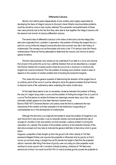
Differential CalculusNewton and Leibniz,quite independently of one another,were largely responsible for developing the ideas of integral calculus to the point where hitherto insurmountable problems could be solved by more or less routine methods.The successful accomplishments of these men were primarily due to the fact that they were able to fuse together the integral calculus with the second main branch of calculus,differential calculus.The central idea of differential calculus is the notion of derivative.Like the integral,the derivative originated from a problem in geometry—the problem of finding the tangent line at a point of a curve.Unlile the integral,however,the derivative evolved very late in the history of mathematics.The concept was not formulated until early in the 17th century when the French mathematician Pierre de Fermat,attempted to determine the maxima and minima of certain special functions.Fermat’s idea,basically very simple,can be understood if we refer to a curve and assume that at each of its points this curve has a definite direction that can be described by a tangent line.Fermat noticed that at certain points where the curve has a maximum or minimum,the tangent line must be horizontal.Thus the problem of locating such extreme values is seen to depend on the solution of another problem,that of locating the horizontal tangents.This raises the more general question of determining the direction of the tangent line at an arbitrary point of the curve.It was the attempt to solve this general problem that led Fermat to discover some of the rudimentary ideas underlying the notion of derivative.At first sight there seems to be no connection whatever between the problem of finding the area of a region lying under a curve and the problem of finding the tangent line at a point of a curve.The first person to realize that these two seemingly remote ideas are,in fact, rather intimately related appears to have been Newton’s teacher,IsaacBarrow(1630-1677).However,Newton and Leibniz were the first to understand the real importance of this relation and they exploited it to the fullest,thus inaugurating an unprecedented era in the development of mathematics.Although the derivative was originally formulated to study the problem of tangents,it was soon found that it also provides a way to calculate velocity and,more generally,the rate of change of a function.In the next section we shall consider a special problem involving the calculation of a velocity.The solution of this problem contains all the essential fcatures of the derivative concept and may help to motivate the general definition of derivative which is given below.Suppose a projectile is fired straight up from the ground with initial velocity of 144 fee t persecond.Neglect friction,and assume the projectile is influenced only by gravity so that it moves up and back along a straight line.Let f(t) denote the height in feet that the projectile attains t seconds after firing.If the force of gravity were not acting on it,the projectile would continue to move upward with a constant velocity,traveling a distance of 144 feet every second,and at time t we woule have f(t)=144 t.In actual practice,gravity causes the projectile toslow down until its velocity decreases to zero and then it drops back to earth.Physical experiments suggest that as the projectile is aloft,its height f(t) is given by the formula.The term –16t2 is due to the influence of gravity.Note that f(t)=0 when t=0 and whent=9.This means that the projectile returns to earth after 9 seconds and it is to be understood that formula (1) is valid only for 0<t<9.The problem we wish to consider is this:T o determine the velocity of the projectile at each instant of its motion.Before we can understand this problem,we must decide on what is meant by the velocity at each instant.T o do this,we introduce first the notion of average velocity during a time interval,say from time t to time t+h.This is defined to be the quotient. Change in distance during time interval =f(t+h)-f(t)/h.ength of time intervalThis quotient,called a difference quotient,is a number which may be calculated whenever both t and t+h are in the interval[0,9].The number h may be positive or negative,but not zero.We shall keep t fixed and see what happens to the difference quotient as we take values of h with smaller and smaller absolute value.The limit process by which v(t) is obtained from the difference quotient is written symbolically as follows:The equation is used to define velocity not only for this particular example but,more generally,for any particle moving along a straight line,provided the position function f is such that the differerce quotient tends to a definite limit as h approaches zero.The example describe in the foregoing section points the way to the introduction of the concept of derivative.We begin with a function f defined at least on some open interval(a,b) on the x axis.Then we choose a fixed point in this interval and introduce the differencequotient[f(x+h)-f(x)]/h.Where the number h,which may be positive or negative(but not zero),is such that x+h also lies in(a,b).The numerator of this quotient measures the change in the function when x changes from x to x+h.The quotient itself is referred to as the average rate of change of f in the interval joining x to x+h.Now we let h approach zero and see what happens to this quotient.If the quotient.If the quotient approaches some definite values as a limit(which implies that the limit is the same whether h approaches zero through positive values or through negative values),then this limit is called the derivative of f at x and is denoted by the symbol f’(x) (read as ―f prime of x‖).Thus the formal definition of f’(x) may be stated a s follows Definition of derivative.The derivative f’(x)is defined by the equation。
《微积分英文》课件 (2)

Types of Limits
One-sided limits
Limits approached
from one direction
Limits at infinity
Behavior of functions at
infinity
● 02
第2章 Limits and Continuity
01 Definition of a limit
Explanation of what a limit is
02 Properties of limits
Key characteristics of limits
03 Calculating limits algebraically
Graphing functions by analyzing their derivatives and key points
Higher Order Derivatives
Second derivative
Rate of change of the rate of
change
nth derivative
● 03
第3章 Differentiation
Derivatives and Rates of
Change
A derivative is defined as the rate of change of a function at a given point. Notation for derivatives includes symbols such as f'(x) or dy/dx. Derivatives can be interpreted as rates of change in various realworld applications.
- 1、下载文档前请自行甄别文档内容的完整性,平台不提供额外的编辑、内容补充、找答案等附加服务。
- 2、"仅部分预览"的文档,不可在线预览部分如存在完整性等问题,可反馈申请退款(可完整预览的文档不适用该条件!)。
- 3、如文档侵犯您的权益,请联系客服反馈,我们会尽快为您处理(人工客服工作时间:9:00-18:30)。
(2)
xn dx
1 n1
x n1
C
(n 1)
(3)
dx x
ln
x
C
( ln x ) 1
x
(4)
1
dx x
2
arctan
x
C
or arccot x C
(5)
dx arcsin x C 1 x2
or
arccos x C
(6) cos xdx sin x C
(7) sin xdx cos x C
Thus
sinn xdx 1 cos x sinn1 x n 1 sinn2 xdx
n
n
x2ex ex 2xdx
x2ex 2 xdex
x2ex 2[xex exdx]
x2ex 2xex ex C
ex x2 2x 2 C
Example5
x ln xdx
3
3
ln
x(
2x2 3
)dx
ln
xd
2x2 3
3
3
2x 2
ln x
2x 2 1 dx
33
udv uv vdu
x2 sin xdx x2d cos x
x2 cos x ccoossxxd(x22x)dx
x2 cos x 2 xd sin x
x2 cos x 2(x sin x sin xdx)
x2 cos x 2xsin x 2cos x C
Example 3 Solution
x ln 2 x
2[
x
ln
x
x
1dx] x
x ln 2 x 2x ln x 2x C
Example9 ex sin xdx exd cos x
ex cos x ex cos xdx
ex cos x exd sin x
ex cos x ex sin x ex sin xdx
Solution Let u x, dv cos xdx,
Then du dx, v sin x
x cos xdx
x sin x sin xdx
xsin x cos x C
udv uv vdu
Example 2 Evaluate x2 sin xdx
Solution
f (x)g(x)]ba
b
f (x)g(x)dx
a
b
f (x)g(x)dx
a
b f (x)g(x)dx
a
f (x)g(x)]ba
b
f (x)g(x)dx
a
or
b udv
a
uv]ba
b
vdu
a
1
1
Exampe
arctan xdx. arctan xdx
0
0
x arctanx 1 0
2
Integration by parts can also be usd in connection With definite integrals,the formula is
b
f (x)g(x)dx
a
f (x)g(x)]ba
b
f (x)g(x)dx
a
b
b
a [ f (x)g(x)] dx a ( f (x)g(x) f (x)g(x))dx
sinn1 x cos x (n 1) (1 sin2 x) sin n2 xdx sinn1 x cos x (n 1) sin n2 xdx
(n 1) sinn xdx
Therefore
n sinn xdx cos x sinn1 x (n 1) sinn2 xdx
f (x)g(x)dx f (x)g(x) f (x)g(x)dx
Let u f (x) and v g(x)
Then the formula for integration by parts becomes
udv uv vdu
Example 1 Find x cos xdx
( f (x)g(x))dx f (x)g(x)dx f (x)g(x)dx
f (x)g(x)dx ( f (x)g(x))dx f (x)g(x)dx f (x)g(x)dx f (x)g(x) f (x)g(x)dx
The formula for integration by parts
2ห้องสมุดไป่ตู้
2
1 x2 1arctan x 1 x C
2
2
Example 7 arccos xdx
x arccos x
x dx
1 x2
x arccos x 1 x2 C
Example 8 ln 2 xdx
xd ln2 x
x ln 2 x
x
2
ln
x
1 x
dx
x ln 2 x 2 ln xdx
xexdx
Evaluate xexdx
xexdx
exd 1 x2
2
xdex
1 x2 ex 1 x2dex
xex exdx 2
2
xex ex C 1 x2 ex 1 x2exdx
2
2
Example 4 Solution
Evaluate x2exdx
x2exdx x2dex
so
ex sin xdx
1 ex sin x cos x C
2
or
ex sin xdx
sin xdex
ex sin x ex cos xdx
ex sin x cos xdex
ex sin x ex cos x ex sin xdx so, ex sin xdx 1 ex sin x cos x C
Chapter 7
Techniques of Integration L’Hospital Rule
and Improper Integrals
7.1 Basic Integration Formulas
Table of Indefinite integrals
(1) dx x C
( C is a constant)
ln a
(14) sh xdx ch x C
sh x ex ex 2
ch x ex ex 2
(15) ch xdx sh x C
Exercise:
2x 9
1.
dx x2 9x 1
2.
dx 8x x2
3. (secx tan x)2 dx
Exercise:
/4
4. 0 1 4 cos4xdx
0
0
(ex sin x ) 2 2 ex cos xdx
0
0
(ex sin x ) 2 0
2 cos xdex
0
e2
(ex
cos x ) 2 0
2 ex sin xdx
0
so
2 ex sin xdx
0
e2
1
2 ex sin xdx
0
Thus
2 ex sin xdx
1
e2
1
0
22
1x 0 1 x2 dx
1 ln(1 x2 ) 1 1 ln 2.
42
0 42
e
Example x ln xdx.
1 e ln xdx2
1
21
1 x2 ln x 2
e 1 e x2 1 dx 1 21 x
e2 2
e2 1 4
1 x2 e
4
1
Example 2 ex sin xdx 2 sin xdex
(8)
dx cos 2
x
sec2
xdx
tan x C
(9)
d sin
x
2
x
csc2
xdx
cot
xC
(10) sec x tan xdx sec x C
(11) csc x cot xdx csc x C
(12) ex dx ex C (13) a xdx a x C
Example Prove the reduction
sinn xdx 1 cos x sinn1 x n 1 sinn2 xdx
n
n
Where n>2 is integer
Proof
sinn xdx sinn1 xd cos x
sinn1 x cos x cos xd sin n1 x sinn1 x cos x (n 1) cos2 x sin n2 xdx sinn1 x cos x (n 1) (1 sin2 x) sin n2 xdx
3x 2
5.
dx 1 x2
6.
3x2 3x
7x 2
dx
7. sec xdx
7.2 Integration by Parts
Integration by Parts If f (x) and g(x) are differentiable functions ,then
( f (x)g(x)) f (x)g(x) f (x)g(x)
3x
2x 2
ln x 33
2 3
xdx
3
2x2 ln x
4x2 C
3
9
Example6 x arctan xdx
arctan
xd
x2 2
arctan x x2 2
x2 2
1
1 x2
dx
x2 2
arctan
x
1 2
1
1
1 x
2
dx