CodeWarrior 10.2简明手册(V1.1)
Freescale CodeWarrior 10.6 集成开发环境(IDE)使用手册
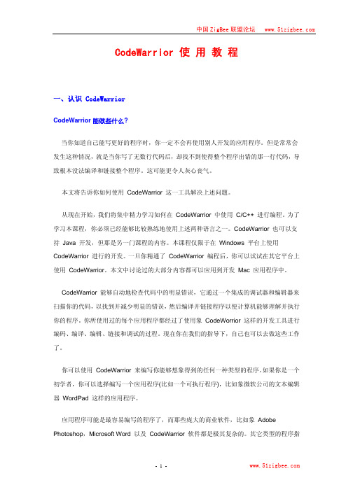
单击此处“…”则会 弹出下页ppt所示的 周期设置窗口
CodeWarrior 10.6 IDE使用手册
14
设置定时器中断周期为10ms
在此输入期望的中断周期10ms 这里列出了当前选择的定时器能 够实现的定时周期及精度 设此处限定定时误差,若设置的中断周 期超出此误差,则处理器专家会报错
CodeWarrior 10.6 IDE使用手册
CodeWarrior 10.6 IDE使用手册
3
利用工程向导快速创建KEA工程
e.选择编程语言和浮点数支持以及控制 台(console)硬件支持: f.选择是否使用处理器专家系统以及工 程外设driver的使用模式:
CodeWarrior 10.6 IDE使用手册
4
利用工程向导快速创建KEA工程
其中包含了默认看门狗、SWD调试口以及Flash Memory 的设置
在CPU组件的属性设置中还包括CPU 内核中断/复位设置(CPU interrupt/reset)
其中包含了CPU内核系统级中断(ARM Cortex M0+实现的 异常):不可屏蔽中断NMI、硬件错误异常Hard fault(当 CPU执行非法指令、非对其地址访问时触发该异常,可以 用于捕获程序跑飞时的场景)、超级调用Supervisor Call和 可请求服务异常(用于RTOS系统任务切换),以及内部时 钟失锁(ICS Loss of lock)。所有这些中断的优先级都高于 外设中断。
CodeWarrior 10.6 IDE使用手册
18
添加和配置定时器中断组件
最后在中断回调函数中添加中断处理,这里为全局中断计数器加1; 注意:用户的中断处理代码必须加在处理器专家指定的位置
CodeWarrior 10.6 IDE使用手册
CODEV10.2说明书1

ALI-Alignment OptimizationALI computes the necessary changes in compensators needed to minimize the differences between nominal design wavefronts and wavefronts measured by an interferometer on the system as-built; these adjustments would then be made in the hardware to restore as much of the design performance as possible. The calculation predicts the potential improvement that making such adjustments will generate, pre- and post-alignment. ALI can also convert a null test interferogram into a surface deformation interferogram.When to Use the Alignment Optimization (ALI) OptionThe ALI option can be used for three purposes:•To predict the small changes in specified parameters (compensators designated in the LDM) needed to do final alignment of an assembled optical system•To predict the potential improvement that making such adjustments will generate, pre- and post-alignment•To convert a null test interferogram into an interferogram measured along the surface normal.The first two are part of the output of the option. The conversion of a null test interferogram to a surface normal interferogram is included here because the computation in ALI is the one needed: defining a system wavefront and relating surface errors to system wavefront errors.The use of ALI should be associated with lens systems that require adjustments after initial assembly. Most rotationally symmetric refractive lens systems are designed to be fabricated and assembled with enough precision that no internal adjustments after assembly are needed; only focus and possibly tilt of the image surface are typically used to enhance performance; an effective tolerance analysis can establish the feasibility of such an approach. Additional steps such as fitting to test plates, melt glass data, or even respacing for measured thicknesses can be applied to give wider latitude to the remaining tolerances or achieve a higher level of quality. These systems do not require the use of the ALI option.In non-rotationally symmetric systems (and even in selected centered systems) it is often too much to expect that all parts can be made and assembled without planning to have final adjustments. For example, multi-mirror unobscured systems depend on adjustable parameters (element tilts and/or displacements) for final tuning of the system to produce the design performance; in fact, they often are designed with 6degree-of-freedom mirror mounts and toleranced with adjustment as an essential step. Alignment would be an impossible task without developing the simultaneous solution for adjustments that the ALI option provides.An assembled system may show residual aberrations not present in the design. Note that - without knowing the magnitude or even the source of specific errors within the lens, but just having the system interferograms at several field angles - computational experiments can be run with this option, trying different potential adjustment scenarios until one is found that restores enough of the design performance. The best scenario can then be applied to do final alignment of the lens assembly.Even some rotationally symmetric systems (e.g., microscope objectives, Cassegrain reflecting systems, etc.) may be designed to have an adjustment (e.g., a mirror tilt, lens element decenter, and/or an airspace) aimed at taking out some residual aberration such as axial coma or spherical aberration; the ALI option makes this a single step process giving both the correct magnitude and direction, instead of a trial-and-error process on the hardware itself. For modest field systems, this often can be done with a single axial system interferogram. In all of the applications suited for treatment by the ALI option, the system must have residual wavefronterrors that can be measured interferometrically.ALI - Alignment OptimizationPreparation for Running the Alignment OptionLike the TOR option, the ALI option calculates wavefront differentials which are linear with respect to the parameter changes. Thus, it can only predict small changes in the user-specified alignment parameters. One common alignment problem is that of rotating two mirrors with respect to each other to minimize the effects of surface errors, e.g., astigmatism. This must be done by assigning the interferogram data to the appropriate surfaces and analyzing the system with any of the image quality options (e.g., WAV). By going through a series of rotation angles (e.g., 0, 30, 60, 90), a minimum may be found.Preparation for Running the Alignment Option For alignment purposes, the lens data should be the best achievable design - the design fitted to glass melt data, test plates and measured thicknesses. Only include enough of these steps, forming the “baseline” design, to represent the design performance as you want it to be post-alignment. Details such as interferometric surface errors are immaterial since the predicted adjustment magnitudes and directions will be unaffected by them; they will only affect the pre- and post-alignment predicted performance.As part of the lens data, include the compensators (CMP) you wish to have used as alignment parameters. These are entered in the LDM (see section on Tolerances). Be sure to include compensators that can be effective in correcting the system (focus shift, image plane tilt or independent focus at each field (INC command), element/subsystem spacings and tilts, etc.). Note that this is a crucial step in the process - selection of the right element decenter in a high numerical aperture microscope objective may make an otherwise unfeasible performance level achievable.There is no limit on the number of compensators allowed, however the best solutions are obtained with the fewest compensators which will accomplish the alignment. The parameters are typically motions of optical elements, such as tilt and decenter of the secondary in a Cassegrain, but also would normally include axial displacement and tilt of the image surface.The focusing mode is determined by compensator entries such as DLZ SI (defocus) and TIL SI (2components of tilt). If none of these compensators is entered, there is no adjustment of the focal surface. With INC (independent compensation), DLZ SI must also be entered if it is to work correctly, but each field will be focused independently and any focal surface tilt compensators will have no effect.A special feature of the ALIgnment option is the ability to calculate the surface deformations of a surface being tested in a null configuration. In some null tests, the surface is not measured at center of curvature, e.g., a parabola in autocollimation. The resulting interferogram, therefore, does not correctly represent surface errors as measured normal to the surface. This feature predicts the correct surface deformations as a Zernike polynomial. To use it, set up the null test configuration as the lens data in the LDM. Run the ALI option, designating the one surface associated with the null test wavefront; write out the .INT file in polynomial form. Repeat for each null tested surface in the system. Then restore the full system and attach the new files to the corresponding surfaces. Proceed with any desired CODE V operations (optimization, evaluation, alignment, etc.).Default OperationNone; no calculation is possible without at least one measured wavefront supplied (INT command). With one such wavefront (measured at the exit pupil for the assembled system in the reference wavelength) entered for each field point and zoom position, values of the small alignment changes are generated. (Alignmentparameters are selected in the LDM as compensators, such as tilts, decenters, axial spacings, and focal plane shift and tilt). The computed changes are those needed to restore as much performance as possible; they are listed along with the RMS error existing before and after alignment. The RMS error is for the difference between the measured and nominal system wavefronts; thus the goal is restoration of design performance, notenhancement relative to a perfect lens. ALI uses Gaussian apodization if present in the lens data.ALI - Alignment OptimizationCommand MnemonicsCommand Mnemonics (alphabetical)Data Input Overview The ALI option assumes that:•The lens data (entered or restored in the LDM) is a system that represents the desired wavefront performance, and that the desired alignment parameters have been designated as compensators in theLDM. Zoom positions can be used to represent a zoom lens or to extend the number of fields at which measurements have been made beyond the limit of 25 for a non-zoom lens.•Exit pupil interferograms have been measured at one or more field points for the hardware assembled as represented in the lens data, and converted to files according to the CODE V standard described in theLDM (several interferometer manufacturers supply this form of output).•These files are attached to their appropriate field points (INT) and scaled in deformation if needed (ISF).The interferograms they represent are matched to the exit pupil in size (INR) and position (FID or IMI, IRO, INX, INY).•All exit pupil interferograms have been measured with respect to images lying on the desired focal surface, or else adjusted so (FOC).•Appropriate values or defaults are present for ray grid density (NRD) and the desired weighting of the various field points (WTF). The default field weights are the LDM field weights.The option then proceeds with its computation. All calculations are done in the reference wavelength only. If it is a null test conversion see “Null Test Computations” on page 21-18 for details. Also see “Discussion of Input and Computations” on page 21-16 for a thorough explanation.FID FOC IMI INR INT INX INY IRO ISF NRD NUL WIN WTF ZFRZRNALI - Alignment OptimizationDefining the InterferogramDefining the Interferogram To define the interferogram, select the Analysis >Fabrication Support > Alignment Optimization menu. The Alignment Optimization dialog box is displayed, with the Interferogram tab in the mand Syntax Screen ControlExplanation Default INT Fk [ Zn ] int_filenameFile Assign system (exit pupil) interferogram data in the file int_filename.INT to field k, zoom n. When more than twenty-five fields are needed, the system may be zoomedto allow other fields (up to 35) to be defined in the added position(s); this is the most frequent use of Zn, althoughzoom systems can also be aligned.None; at least one interferogram isREQUIRED.ISF Fk scale_factor....zScale Scale the measured wave deformation for field k anddesignated zoom position by the specified scale factor -provides a convenient scale factor separate from the one specified in the interferogram file. Example : use 0.5 for scaling of wavefront data measured in a double-pass test.1.0.ALI - Alignment Optimization Defining the Interferogram INR Fk radius....z Radius Radius of data on the exit pupil at field k and designatedzoom position, in units of the lens. This connects the unit length of the file data to a physical length on the exit pupil. The unit length of file data is defined:Zernike polynomials–In a circle of unit radius Grid –In a square of unitsemi-dimension The entered value of physical length is the radius on the exit pupil, measured in a direction normal to the chief ray.Note : If the given value of radius scaled theinterferogram smaller than needed to cover the exit pupil, the data outside the unit semi-dimension will eitherbe missing (grid) or extrapolated (polynomial) leading to false results; this must be avoided.Semi-diameter of the exit pupil.IMI Fk XC | YC | No....zMirror Mirror image in X or Y at field k and designated zoom position:XC –Move deformation data to theopposite X-coordinateYC –Move deformation data to theopposite Y-coordinateN or No – No mirror image is doneOnly one of IMI XC or IMI YC can be done at a given field position; to do both is equivalent to an IRO of 180°.No.INX Fk x_dec....zX Decenter The X coordinate for the interferogram center in the plane containing the exit pupil point and normal to the chief ray, at field k and designated zoom position.Chief rayintersection.INY Fk y_dec....zY Decenter The Y coordinate for the interferogram center in the plane containing the exit pupil point and normal to the chief ray, at field k and designated zoom position.Chief rayintersection.IRO Fk ang_rot_degr....zRotation Angle of rotation, in degrees, of the deformation data in the interferogram at field k and designated zoom position. Rotation is about the center of the interferogram. Rotation of the positive X axis toward the positive Y axis(counterclockwise) is a positive rotation. If IMI was entered, the IRO action is done after IMI.0.0Command Syntax Screen Control Explanation DefaultALI - Alignment OptimizationFitting the Interferograms to the Exit PupilFitting the Interferograms to the Exit PupilOrienting Interferogram DataFive commands are available for orienting interferogram data on the exit pupil in this option:FID Fk [ Zn ] x_R2 y_R2 x_R3 y_R3 [ x_R4 y_R4 [ x_R5 y_R5 ] ]Fiducials for interferogram data alignment w.r.t. reference ray Fiducials for aligning the interferogram data at field k, zoom n with the CODE V reference rays. Values are points relative to the unit circle (of the interferogram) where the CODE V reference rays (R2, R3, R4 and R5) pass through the interferogram (assuming it is positionedin the real exit pupil, normal to the chief ray). The action is dependent on the number of rays referenced in the X_Rn, Y_Rn values:R2, R3MINIMUM DATA. Generatesvalues for rotation (IRO), scaling(INR), and decenter in X and Y(INX, INY) to match exactly the4 values.R2, R3, R4, orR2, R3, R4, R5Generates values for mirrorimage (IMI,XC),rotation (IRO),scaling (INR), image (IMI, XC),and decenter in X and Y (INX,INY) that minimizes in the least squares sense the departures fromthe 6 (or 8) values.None. Uses IMI, IRO, INR, INX, mand Description LocationIMI Reverse interferogram data “left-for-right” or “up-for-down” (i.e., a mirror image in X or Y, respectively)Interferogram tab (See “Defining the Interferogram” on page 21-8.)IRO Rotate the interferogram about its center Interferogram tab (See “Defining the Interferogram” on page 21-8.)INR Scale the interferogram unit dimension to the specified value Interferogram tab (See “Defining the Interferogram” on page 21-8.)INX, INY Shift center point of interferogram to a designated X, Y point in the exit pupil Interferogram tab (See “Defining the Interferogram” on page 21-8.)Command Syntax Screen Control Explanation DefaultALI - Alignment OptimizationFitting the Interferograms to the Exit PupilIMI and IRO apply to interferogram coordinates only. The interferogram coordinate system is:IMI XC means that data that was on the +X side is now on the -X side and vice versa. IMI YC has a similar meaning in the Y direction. Notice that it is the deformation data that moves; the axes do not move. IRO rotates the data by the specified angle, where counterclockwise is the positive direction (rotating the positive X axis toward the positive Y axis). If both IMI and IRO are entered, the IMI is done first.INX, INY and INR apply to the exit pupil only. INX and INY specify where the center of the interferogram is placed. These are given in units of the lens system. INR is the radius of the data, also in lens units. It equates the unit radius of the interferogram data to a physical distance.Mirror Image, Rotation, and Translation OrderThe transformations IMI, IRO, INX and INY are performed in the order of: mirror image, rotation,translation.Defaults apply:•The interferogram is centered on the intersection of the chief ray with the exit pupil. Overridden by FID, INX and/or INY.•No mirror image. Overridden by FID and/or IMI.•No rotation. Overridden by FID and/or IRO.•The radius of the data is the semi-diameter of the exit pupil. Overridden by FID and/or INR.Interferograms which are entered in ALI, are associated with the exit pupil. The coordinates of the exit pupil are always measured perpendicular to the chief ray. This is because an interferogram represents the image of the exit pupil of the system and the axis of the interferometric setup is approximately along the chief ray. The coordinates of the interferogram are mapped onto the plane which is tangent to the reference sphere at the position where the chief ray intersects the reference sphere.An alternate method of orienting the interferogram to the exit pupil is by matching fiducial points on the interferogram to the intersection of the CODE V reference rays with the tilted exit pupil. The CODE V reference rays are used to define the bundles of light. These rays are:Ray Label DescriptionR1Chief rayR2Upper (+) Y rayR3Lower (-) Y rayR4“Upper” (+) X rayR5“Lower” (-) X rayALI - Alignment OptimizationNull Test Analysis: Converting Non-normal Null Test Interferograms to Normal InterferogramsThe FID input defines between two and four points on the interferogram which are associated with the reference rays, R2, R3, R4 and R5. If only two points (R2, R3) are used, an exact fit can be obtained; for more than two points, a least squares fit is done between the fiducial points and the intersection of the CODE V reference rays with the tilted exit pupil. The solution gives the values of IMI, IRO, INR, INX and INY.If a set of fiducial points (FID) is entered, it will be used for the referencing. Otherwise, the specific coordinate transformations (IMI, IRO, INR, INX, INY) or their defaults will be used. Null Test Analysis: Converting Non-normal Null Test Interferograms to Normal Interferograms In some null tests, the lens surface is not measured at its center of curvature; for example, a parabola could be tested at its focus with a flat mirror. The resulting interferogram, therefore, does not directly represent surface errors as measured normal to the surface. Since surface errors, as specified in .INT files, are assumed to be measured along the surface normal, a way is needed to convert the results of a non-normal null test to surface deformations along the surface normal. This is done, on one interferogram at a time, as follows:•Set up the single field null test configuration as your lens, in the LDM, then enter this option (ALI) •Use INT to place the null test interferogram in the exit pupil•Use ISF, FID or IMI, IRO, INR, INX, INY as necessary•Use NUL to bypass regular alignment operations and to convert the exit pupil interferogram into a surface interferogram for the designated surface•Use ZRN or ZFR to designate form of Zernike polynomial to be generated•Use NRD if necessary to provide enough grid points for the single field fit to polynomials of the designated order•Use WIN (writes the information on a file in a format compatible with the INT command in the LDM) •Do the same for any other surfaces measured by null test interferogramsSet up your actual optical system in the LDM, attaching these new surface interferograms to the assigned surfaces plus any other surface interferograms. Proceed with any desired CODE V operations (optimization,evaluation, etc.).ALI - Alignment Optimization Defining a Null Test Analysis Defining a Null Test Analysis To define a null test analysis, select the Analysis >Fabrication Support > Alignment Optimization menu. The Alignment Optimization dialog box is displayed. Select the Null Test tab to bring it to the foreground. Command SyntaxScreen Control Explanation DefaultNUL Sk [ radius ]Surface number for null test /Radius of surface (lensunits)Bypass the normal alignment calculation and convert the one exit pupil interferogram from a null test into a surface interferogram for surface Sk. The lens must bethe optical system representing the null test; one, and only one, exit pupil interferogram (INT) must beentered. The ray traced wavefront is compared to themeasured exit pupil interferogram; any differences are assumed to be due to errors on the specified surface. A Zernike polynomial fit is done to the surfacedeformations, specified by the ZRN or ZRF command;if neither is given, ZRN 36 is used. The unit circle for the polynomial corresponds to the radius entered on theNUL command. If a radius is not entered, the clear aperture of surface Sk is used.Do the normal alignment process.ALI - Alignment OptimizationDefining a Null Test AnalysisZRN num_terms Select Interferogram Format: StandardZernike Use with NUL. Fit the residual system wavefront, from the null test configuration, to a standard Zernike polynomial to be used as a surface deformation. The fit is done with respect to normalized exit pupilcoordinates, but centered on and measured in a direction normal to the chief ray. Either ZFR or ZRN may be entered but not both. 36, if NUL is used.ZFR num_termsSelect Interferogram Format: Fringe Zernike /Number of terms Use with NUL. Fit the residual system wavefront, from the null test configuration, to a FRINGE Zernike polynomial to be used as a surface deformation. The fit is done with respect to normalized exit pupilcoordinates, but centered on and measured in a direction normal to the chief ray. Either ZFR or ZRN may be entered but not both.None. Use ZRN.WIN int_filenameEnter interferogram file name for saving Zernike coefficients Use with NUL. For the residual system wavefront, from the null test configuration, write Zernike coefficients on an interferogram file namedint_filename.INT, for use as a surface deformation.No file mand Syntax Screen Control Explanation DefaultDefining Computation ControlsDefining Computation ControlsTo define computation controls, select the Analysis >Fabrication Support > Alignment Optimization menu. The Alignment Optimization dialog box is displayed. Select the Computation tab to bring it to the foreground.Command SyntaxScreen ControlExplanationDefaultNRDnum_rays_across_diameter Number of rays across diameterNumber of rays traced across the pupil diameter at each wavelength. Recommendation: There should be enough rays to give a reasonable representation of theaberrations for the RMS calculation. The default is sufficient in most cases. For significant vignetting and/or central obscuration, increase NRD. For the NUL analysis, the smoothness of fit to Zernikepolynomials is dependent on having significantly more (at least twice as much) information than the number of terms in the polynomial. Increase NRD if number of terms is high, especially with significant vignetting and/or central obscuration.16.Discussion of Input and ComputationsDiscussion of Input and ComputationsWhat to Include in the LDM Lens DataFor alignment purposes, the lens data should be the best achievable design – the design fitted to glass melt data, test plates and measured thicknesses. Only include enough of these steps, forming the “baseline” design, to represent the design performance as you want it to be post-alignment. On the other hand, don't expect the option to overcome the effects of severe, unadjustable errors; the process only aims to minimize the difference between the baseline design and the post-alignment system; if the baseline design is too far away from what is achievable with the adjustment parameters given, the balance may not be optimum. Details such asinterferometric surface errors are immaterial since the predicted adjustment magnitudes and directions will be unaffected by them; they will only affect the pre- and post-alignment predicted performance.As part of the lens data, include the compensators (CMP) you wish to have used as alignment parameters. Values entered with the compensators (or their defaults) act as limits to the allowed changes. Be sure to include compensators that can be effective in correcting the system (focus shift, image plane tilt orindependent focus at each field (INC command), element/subsystem spacings and tilts, etc.). Note that this is a crucial step in the process - selection of the right element decenter in a high numerical aperture microscope objective may make an otherwise unfeasible performance level achievable.Specific tolerancing controls allow ALI to select the most effective set of compensators for your system. The Singular Value Decomposition (SVD) Threshold and Used Compensators controls in the System Data window (SVT and MCP commands, respectively) regulate the compensators used to align the system. See “Defining Tolerance Controls” on page 3-60 for details about these commands. In addition, you can specify which compensators must be used, and which can be dropped from the system. This is done using the Compensator Use Control field in the Surface Properties window, on the Tolerances page. From the command line, use the CMP command. For details, see the CMP command description under “Other Tolerance Controls” on page 8-23.WTF field-zoom_weight....f, zField Weights forBalancing Alignment SolutionField weights to balance for solution of alignment parameters. If field_zoom_weight value is 0, computations for that field will be skipped.Lens system weightsfrom WTF in the LDM.FOC focal_shift....f, z Wavefront Focal ShiftFocal shift added to the lens at the specified field/zoom position. Use to compensate for focal shifts known to be present in the measured system interferograms, and to bring them, as needed, into acommon reference with respect to the focal surface as defined in the lens data. Note : Needed so that the focus compensation arrangement defined in the LDM is applied correctly; otherwise, focus compensator values will apply to the unrelated (and possibly unknown) foci represented in the system interferograms.0.0Command SyntaxScreen ControlExplanationDefaultDiscussion of Input and ComputationsUsageThe ALI option predicts small changes in specified alignment parameters based on measured wavefront data at one or more fields:•It uses the baseline design as the performance standard, and compensators (CMP) to designate the alignment parameters, entered in the LDM•It uses measured system wavefront data entered in the option itself•Predicted changes in the alignment parameters are used for adjusting the hardware.Figure 2.Schematic of the ALI optionMore specifically, the ALI option assumes that:•The lens system (entered in the LDM or restored) has been optimized to represent the quality standard to be used, and that the desired alignment parameters have been designated as compensators in the LDM. Zoom positions can be used to represent a zoom lens or to extend the number of fields at whichmeasurements have been made beyond the limit of 25 for a non-zoom lens.•Exit pupil interferograms have been measured at one or more field points for the hardware assembled as represented in the lens data, and converted to files according to the CODE V standard described in theLDM (several interferometer manufacturers supply this form of output).•These files are attached to their appropriate field points (INT) and scaled in deformation if needed (ISF ). The interferograms they represent are matched to the exit pupil in size (INR ) and position (FID or IMI , IRO , INX , INY ).•All exit pupil interferograms have been measured with respect to images lying on the desired focal surface, or else adjusted so (FOC ).•Appropriate values or defaults are present for ray grid density (NRD ) and the desired weighting of the various field points (WTF ). The default field weights are the LDM field weights.。
FreescaleCodeWarrior10.6集成开发环境(IDE)使用用户手册

e.选择编程语言和浮点数支持以及控制 台(console)硬件支持:
f.选择是否使用处理器专家系统以及工 程外设driver的使用模式:
CodeWarrior 10.6 IDE使用手册
4
利用工程向导快速创建KEA工程
处理器专家系统工程介绍 工程及文件窗口
处理器专家为
每一个组件 (compontent) 生一个对应 的.h和.c文件, 包含该组件图
Freescale CodeWarrior 10.6 集成 开发环境(IDE)使用手册
本手册详细介绍了利用Freescale CodeWarrior 10.6 IDE 处 理器专家系统(Processor Expert)快速建立KEA工程和调试的 步骤,以及该IDE常用的编程及调试技巧,旨在帮助用户快速 熟悉和掌握CodeWarrior 10.6的使用,利用处理器专家系统快 速搭建应用工程进行产品原型验证。
CodeWarrior 10.6 IDE使用手册
2
利用工程向导快速创建KEA工程
c. 选择器件,这里KEA属于Kinetis E系列, d. 选择调试工具,这里必须选择TRK-KEA128板
故选择如下:
载的OpenSDA作为本工程的调试工具:
CodeWarrior 10.6 IDE使用手册
3
利用工程向导快速创建KEA工程
6
CPU组件介绍及配置
在CPU组件的属性设置中还包括常
规设置(common settings)
其中包含了默认看门狗、SWD调试口以及Flash Memory 的设置
在CPU组件的属性设置中还包括CPU
内核中断/复位设置(CPU
interrupt/reset)
其中包含了CPU内核系统级中断(ARM Cortex M0+实现的 异常):不可屏蔽中断NMI、硬件错误异常Hard fault(当 CPU执行非法指令、非对其地址访问时触发该异常,可以 用于捕获程序跑飞时的场景)、超级调用Supervisor Call和 可请求服务异常(用于RTOS系统任务切换),以及内部时 钟失锁(ICS Loss of lock)。所有这些中断的优先级都高于 外设中断。
C语言重点语法及CodeWarrior使用介绍
的在线调试功能,可实现程序下载,单步/全速运行,可以设若干个断点,可 以观察和修改任意寄存器或 RAM 内存空间。BDM 几乎是开发飞思卡尔 8 位 (9S08 和 RS08 系列)、16 位(9S12 系列)和 32 位(Coldfire V1 系列)单片
快速实现芯片初始化代码的自动生成工 作,而且 PE 还提供了大量的软件库可供 用户开发时嵌入或调用。因为 8 位单片机
结构和功能相对简单,实现的控制项目复
杂度也不是很高,故一般情况下 8 位机开 发我们都不需要 PE 的介入,自己直接编
图 1-6
写程序代码即可。关于 PE 的详细介绍将
耗费大量的文字,这里按下不提。所以在 图 1-6 的对话框中选择“None”,并直接 按“Next”进入下一步。
如果你以前编写了很多代码文件现在想重 复利用,那么可以通过图 1-5 对话框左面
的文件树选择对应的文件,按中间的
“ Add ” 逐 个 添 加 到 右 侧 的 “ Project Files ” 列 表 中 。 若 加 错 了 就 用 “Remove”把列表中的文件移除。注意 此列表下方的两个选项:“Copy files to project”选择是否将所选的文件拷贝到现
这是项目建立模板的最后一步。在这一步
你可以决定有关 C/C++的一些编译和代码 生成模式,见图 1-7。 启动代码选择。所有 C 编译器会自动
生成一些启动代码。单片机复位后的
指令运行将首先执行这些启动代码, 然后再进入到你自己的程序模块 main
函数。这些启动代码主要完成堆栈指
针初始化、全局和静态变量自动清零
CodeWarriorV.软件使用指南
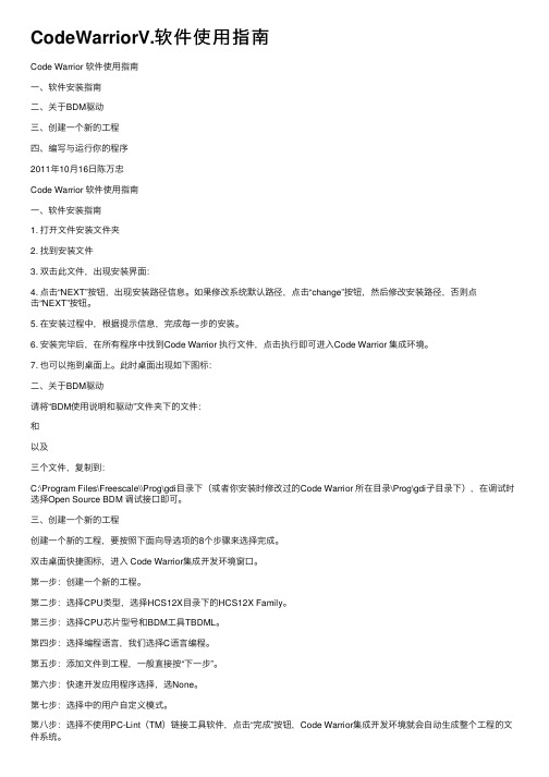
CodeWarriorV.软件使⽤指南Code Warrior 软件使⽤指南⼀、软件安装指南⼆、关于BDM驱动三、创建⼀个新的⼯程四、编写与运⾏你的程序2011年10⽉16⽇陈万忠Code Warrior 软件使⽤指南⼀、软件安装指南1. 打开⽂件安装⽂件夹2. 找到安装⽂件3. 双击此⽂件,出现安装界⾯:4. 点击“NEXT”按钮,出现安装路径信息。
如果修改系统默认路径,点击“change”按钮,然后修改安装路径,否则点击“NEXT”按钮。
5. 在安装过程中,根据提⽰信息,完成每⼀步的安装。
6. 安装完毕后,在所有程序中找到Code Warrior 执⾏⽂件,点击执⾏即可进⼊Code Warrior 集成环境。
7. 也可以拖到桌⾯上。
此时桌⾯出现如下图标:⼆、关于BDM驱动请将“BDM使⽤说明和驱动”⽂件夹下的⽂件:和以及三个⽂件,复制到:C:\Program Files\Freescale\\Prog\gdi⽬录下(或者你安装时修改过的Code Warrior 所在⽬录\Prog\gdi⼦⽬录下),在调试时选择Open Source BDM 调试接⼝即可。
三、创建⼀个新的⼯程创建⼀个新的⼯程,要按照下⾯向导选项的8个步骤来选择完成。
双击桌⾯快捷图标,进⼊ Code Warrior集成开发环境窗⼝。
第⼀步:创建⼀个新的⼯程。
第⼆步:选择CPU类型,选择HCS12X⽬录下的HCS12X Family。
第三步:选择CPU芯⽚型号和BDM⼯具TBDML。
第四步:选择编程语⾔,我们选择C语⾔编程。
第五步:添加⽂件到⼯程,⼀般直接按“下⼀步”。
第六步:快速开发应⽤程序选择,选None。
第七步:选择中的⽤户⾃定义模式。
第⼋步:选择不使⽤PC-Lint(TM)链接⼯具软件,点击“完成”按钮,Code Warrior集成开发环境就会⾃动⽣成整个⼯程的⽂件系统。
四、编写与运⾏你的程序在Code Warrior集成开发环境中,利⽤其⾃动⽣成的函数模板,就可以编写和调试你的应⽤程序了。
codewarrior使用指南
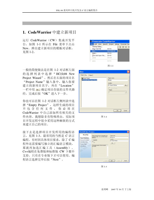
1、安装 CodeWarrior 软件 安装 CodeWarrior 所需要的电脑的硬件资源如下,目前一般的电脑都可以满足这个要求。
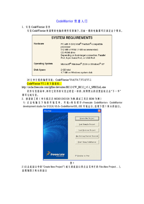
16 位单片机的编程环境:CodeWarrior V4.6,V4.7,V5.0,V5.1 CodeWarrior V5.1 的下载链接: /lgfiles/devsuites/HC12/CW_HC12_v5.1_SPECIAL.exe 软件安装很简单,和其它软件的安装过程是一样的,按照默认的设置直接点击“下一步” 即可完成安装。 2、创建新工程(单片机以以 MC9S12XS128 为例,调试工具以 BDM 为例) 1) 点 击电 脑 左下 角 的 开始 菜 单, 开 始 >所 有 程 序>Freescale CodeWarrior> CodeWarrior development studio for S12(X) V5.0> CodeWarriorIDE。IDE 开始运行,出现下图 1 所示的窗口。
图11
图12 接下来给核心板供电,核心板的供电电压是 5V。有的 BDM 有 5V 供电模式,这个时候 直接用 BDM 供电就可以。 2)在新建的工程中键入如下代码 #include <hidef.h> #include "derivative.h" #define LEDCPU PORTK_PK4 #define LEDCPU_dir DDRK_DDRK4 void delay(void) { unsigned int i; for(i=0;i<50000;i++); } void main(void) { LEDCPU_dir=1; EnableInterrupts;
图8
Codewarrior使用指南

Codewarrior使用指南Codewarrior 使用指南飞思卡尔 HC08/HCS12 系列微控制器开发环境 - Codewarrior 使用指南(草稿)tyf01@/doc/ab18307025.html, 2005 年 10 月仅供学习参考,请勿用于商业目的1Codewarrior 使用指南第一章 Codewarrior IDE 概述在软件开发过程中,通常需要经过以下几个步骤:? 新建:创建新项目,源文件? 编辑:按照一定的规则编辑源代码,注释? 编译:将源代码编译成机器码,同时还会检查语法错误和进行编译优化? 链接:将编译后的独立的模块链接成一个二进制可执行文件? 调试:对软件进行测试并发现错误在软件开发中,每个过程都会用到不同的工具。
如果每个工具都单独存在,这样就会给开发人员带来很多不便。
所以很多公司为开发人员提供了集成开发环境。
开发人员可以在同一个工具或平台上完成以上全部的工作。
Codewarrior 是 Metrowerks 公司开发的软件集成开发环境(以后简称IDE)。
飞思卡尔所有系列的微控制器都可以在 codewarrior IDE 下进行软件开发。
Codewarrior IDE 特点Codewarrior IDE 为软件开发提供了一系列的工具,其中包括:项目管理器:为软件开发人员管理上层的文件;将项目进行分组管理,比如文件或目标系统;跟踪状态信息,比如修改日期;决定编译顺序或每次编译应包括哪些文件;与插件一起提供版本控制功能编辑器:利用颜色来区分不同的关键字;允许用户利用颜色机制自定义关键字;自动检查括号范围;利用菜单在不同的文件或函数中导航搜索器:搜索一个特定的字符串;用特定的字符串代替查找到的字符串;允许使用常规表达式;提供文件比较功能;源代码浏览器:标志符(变量名称,函数名称)数据库;利用数据库来对代码快速定位;对所有的标志符连接到用到它的代码中;编译系统:编译器将源代码编译成机器码;链接器将目标文件链接成可执行文件调试器:利用标志符数据库进行源代码级调试;支持各种标志符数据库,比如:codeview, DWARF, SYM 等Codewarrior IDE 优点交叉平台开发2Codewarrior 使用指南开发人员可以在不同的操作系统下使用codewarrior IDE 来开发自己的软件。
CodeWarrior使用教程
CodeWarrior 使 用 教 程一、认识 CodeWarriorCodeWarrior 能做些什么?当你知道自己能写更好的程序时,你一定不会再使用别人开发的应用程序。
但是常常会发生这种情况,就是当你写了无数行代码后,却找不到使得整个程序出错的那一行代码,导致根本没法编译和链接整个程序。
这可能更令人灰心丧气。
本文将告诉你如何使用 CodeWarrior 这一工具解决上述问题。
从现在开始,我们将集中精力学习如何在 CodeWarrior 中使用 C/C++ 进行编程。
为了学习本课程,你必须已经能够比较熟练地使用上述两种语言之一。
CodeWarrior 也可以支持 Java 开发,但那是另一门课程的内容。
本课程仅限于在 Windows 平台上使用 CodeWarrior 进行的开发。
一旦你精通了 CodeWarrior 编程后,你可以试试在其它平台上使用 CodeWarrior。
本文中讨论过的大部分内容都可以应用到开发 Mac 应用程序中。
CodeWarrior 能够自动地检查代码中的明显错误,它通过一个集成的调试器和编辑器来扫描你的代码,以找到并减少明显的错误,然后编译并链接程序以便计算机能够理解并执行你的程序。
你所使用过的每个应用程序都经过了使用象 CodeWorrior 这样的开发工具进行编码、编译、编辑、链接和调试的过程。
现在你在我们的指导下,自己也可以去做这些工作了。
你可以使用 CodeWarrior 来编写你能够想象得到的任何一种类型的程序。
如果你是一个初学者,你可以选择编写一个应用程序(比如一个可执行程序),比如象微软公司的文本编辑器 WordPad 这样的应用程序。
应用程序可能是最容易编写的程序了,而那些庞大的商业软件,比如象 Adobe Photoshop,Microsoft Word 以及 CodeWarrior 软件都是极其复杂的。
其它类型的程序指的是控制面板(control panels),动态链接库(dynamic linked libraries,DLLs) 和插件(plug-ins)。
- 1、下载文档前请自行甄别文档内容的完整性,平台不提供额外的编辑、内容补充、找答案等附加服务。
- 2、"仅部分预览"的文档,不可在线预览部分如存在完整性等问题,可反馈申请退款(可完整预览的文档不适用该条件!)。
- 3、如文档侵犯您的权益,请联系客服反馈,我们会尽快为您处理(人工客服工作时间:9:00-18:30)。
CodeWarrior 10.2简明手册CodeWarrior 10.2简明手册 (1)1 下载安装CW v10.2 (1)2 安装BDM驱动 (2)3 导入现有工程 (3)4 编译、下载源码工程 (4)5. 带有操作系统程序的编译、下载 (6)5.1 带有操作系统模板程序的打开 (6)5.2 带有操作系统模板程序的编译 (7)5.3 带有操作系统模板程序的下载 (7)6 CodeWarrior 10.2常用操作 (8)7 常见问题说明 (9)基于Eclipse的CodeWarrior Development Studio for Microcontroller v10.2(简称CW10.2)作为一个完整的集成开发环境,提供了高度可视化操作及自动创建复杂嵌入式系统应用的功能,为使用Freescale嵌入式产品开发提供了便利。
官方推荐使用CW v10.2进行Freecale Kinetis嵌入式产品的开发。
本文将对使用CW v10.2开发K60项目的操作进行简要说明。
本文安装的cw10.2 版本是特别版的,支持128KB的代码大小。
用户若需要更大的代码空间和更多的功能的话,则需要向飞思卡尔申请license,这些license都是要收费的。
1 下载安装CW v10.2飞思卡尔半导体为注册用户在其官方网站的网址链接处下载后,双击可执行安装文件,如图1所示,根据提示即可完成安装。
由于有的CW10.2版本安装完成后默认是中文版的,有的默认是英文版的。
集成开发环境的原版是英文版的,所以英文版的运行速度比中文版的快很多。
这里建议用英文版的CW10.2,不建议用户使用中文版集成开发环境,所以本章介绍的使用说明都是基于英文版的。
想将飞思卡尔的CW10.2集成开发环境变成英文版,首先需要关闭当前的CW10.2,然后右击CW10.2桌面图标选择“属性”,在“目标”栏下“…”后面加上“–nl en”再单击“应用”后便改成英文版;加上“–nl zh”可以改2 安装BDM驱动CW_v10.2中已包含了BDM写入器(Open Source BDM,OSBDM)的驱动文件,将BDM接到PC机器时,Windows会提示发现新硬件:提示连接到“Windows Update”更新,选择“否,暂时不”,点击“下一步”。
提示系统自动安装向导,选择“自动安装软件”,点击“下一步”。
安装“PEMicro USB Serial Port”与安装“Open Source BDM”过程相同。
至此,BDM驱动安装过程结束。
3 导入现有工程在Windows XP下,选择“开始”->“所有程序”->“Freescale CodeWarrior”->“CW for MCU v10.2”->“CodeWarrior”启动CW10.2。
启动CW10.2时,提示选择工作空间,可使用默认。
选择“File”->“Import...”,出现导入文件对话框,选择“General”常规分组中的“Existing Projects into Workspace”,点击“Next”。
在“Brose…”导入项目对话框中,选中工程目录(即程序所在最里一层的根目录,例如D:\Ch03-PRG(GPIO-Light)\Ch03-GPIO(Light)\Light),在“Projects”面板中会出现IDE图3 导入项目对话框导入的过程中可能会提示4次关于添加远程系统引用的提示信息,这是关于BDM的引用声明,均点击“是”即可。
另外还有一种简单的方法,找到工程目录最里一层的工程文件夹,例如上例的“D:\Ch03-PRG(GPIO-Light)\Ch03-GPIO(Light)\Light)”文件,直接拖入CW10.2的代码编辑框内便可自动打开工程,一般使用此种方法打开工程较为简便。
4 编译、下载源码工程导入已有工程成功之后,重新对工程进行创建,可下载生成机器码文件下载到MCU 中。
菜单栏中选定“Project”->“Build Configrations”->“Set Active”->“MK60N512VMD100_INTERNEL_FLASH”,设定当前创建的是要写入到目标芯片Flash 的项目,如图4所示。
图4 设置当前活跃项目为写入Flash选择“Project”->“Clean...”,出现清理对话框,选择清理工程(例如“Ch03-GPIO(Light)”)。
同时,勾选“Clean projects selected below”,“Build only the selected project”,点击“OK”,由于编译环境从cw10.1变成了cw10.2,相应的写入器固件程序也得升级。
利用苏州大学“飞思卡尔Kinetis微控制器写入器”写程序时,若写入器不升级,将无法将程序写入芯片中,将出现图6所示的升级提示。
将苏州大学飞思卡尔Kinetis微控制器写入器上的J10两脚的短排针焊接上,并给它加上跳线帽(没有跳线帽和短排针用导线将两个引脚短接即可)。
重新插拔USB接口,点击图6提示对话框的“OK”按钮。
用户只需等待几分钟便可以升级完成。
完成后拔掉J10接口上的跳线帽,重新连接USB线供电,便可以写入程序了。
点击工具栏中的“下载”工具图选中“Flash File To Target”,出现编程下载对话框。
选择运行配置为“K60_MK60N512VMD100_INTERNEL_FLASH_PnE OSJTAG”;选择“Flash Configuration”为“MK60N512VMD100”其它选项不做修改。
选择“Workspace...”,从工程组织下选择“MK60N512VMD100_INTERNEL_FLASH”分组下“Source”的“xxx.afx”(或xxx.afx.s19、xxx.afx.hex任一亦可)文件,载入生成机器码文件。
选择“Erase and Program”,即可完成下载程序到MCU中,如图8所示。
图8 写入程序选项5. 带有操作系统程序的编译、下载5.1 带有操作系统模板程序的打开飞思卡尔实验室为用户设计了基于K60N512芯片的MQX的模板工程,下面讲解飞思卡尔MQX模板工程在CodeWarrior10.2集成开发环境下的打开、编译与下载过程。
首先将带有MQX程序的模板工程目录放在英文目录下。
注意CodeWarrior 10.2同CodeWarrior 10.1一样CodeWarrior 10.2的编译器只能编译英文目录下的工程,不然会出现编译错误,从而导致MQX模板工程不能通过编译。
模板工程的文件组织与Freescale MQX 3.8默认的安装目录下样例工程的结构类似,各目录的简要功能如图80-9所示。
MQX的BSP工程、PSP工程和APP工程(应用工程)在..\mqx_k60n512\mqx\build\cw10目录下,对带有操作系统的程序模板工程文件便是这3个文件,读者对模板工程程序的操作都只是针对这3个文件而言的。
MQX模板工程组织如图9所示。
带有操作系统程序的打开方法与不带操作系统的程序一样,具体参见第3节“导入现有工程”,可分为三个步骤。
第一步:将..\mqx\build\cw10\psp_sdk60n512下的PSP工程按照第3节中的方法拖入CodeWarrior 10.2中。
第二步:将..\mqx\build\cw10\bsp_sdk60n512下的BSP工程按照第3节中的方法拖入CodeWarrior 10.2中。
第三步:..\mqx\build\cw10\app_sdk60n512下的用户工程按照第3节中的方法拖入CodeWarrior 10.2中。
这样带有操作系统的程序便全部加载进CodeWarrior 10.2集成开发环境了,下面便是5.2 带有操作系统模板程序的编译编译的方法与第4节的方法一样,注意编译的顺序应该为PSP工程、BSP工程、APP 工程,先后顺序不能颠倒,不然很有可能出现编译错误的情况。
编译成功完后,BSP、PSP工程的编译生成文件将在“..\mqx_k60n512\lib”路径文件下。
APP工程生成的S19格式的文件将在APP工程自己的目录下“..\mqx_k60n512 \mqx\build\cw10\app_k60n512\twrk60n512_Int_Flash_Debug”文件夹下生成。
5.3 带有操作系统模板程序的下载将5.2节中最后编译APP工程生成的S19文件写进K60N512的芯片中,写入的方法如第4节相同。
至此带有操作系统模板程序的打开、编译、下载便全部完成了。
6 CodeWarrior 10.2常用操作1.查看函数、宏定义原型在利用CW10.2查看代码的过程中若想查看函数或者宏定义的原型,把光标定位到函数、宏定义上,单击右键点击“Open Declaration”或直接按“F3键”便可。
2.查找利用CW10.2集成开发环境在整个工程的所有文件中查找某个关键字,在菜单栏的“Search”下选择“Search”选项。
在跳出的Search对话框中的“Containing text”下输入搜索内容,在“File name patterns”下点击“choose”选择要在什么文件内查找搜索框内的字符(一般选.c和.c文件即可),最后单击“Search”按钮完成搜索。
如图10所示。
在搜索完成后再CW10.2运行界面的右边部分会出现搜索的结果,单击依次查询搜索3.在工程中添加文件与文件引用1)添加文件方法一:点击工程名单击右键现则“Add Files”,在对话框中找到要添加的文件选择“打开”按钮。
在单击“打开”按钮后,选择“Copy files”是将添加的文件复制到工程物理目录下。
选择“Link files”是将文件链接到工程内,添加的文件本身还在原来的物理路径下。
使用方法一时建设使用“Copy files”添加文件。
方法二:将要添加的文件复制到要放入的工程目录下,然后在CW10.2下,点击工程名,右击工程名点击“Refresh”,文件便会自动加进工程。
这里推荐使用第二种方法添加一个文件。
2)添加文件引用利用上述方法虽然将文件加进了工程,但CW 10.2并未将文件“引用”,需要添加工程应用,这样头文件见才能将其包含至工程。
在CW10.2下点击工程名,右击后点击“Properties”,在左边栏点击“C/C++ Build”下选择“Settings”。
在“Setting”右边的选项卡内选择“Tool Settings”下的“ARM Compiler”中的“Input”项,然后在“Include UserSearch Paths (-i)”单击选择“Workspace…”添加工程路径单击“OK”便可。