计量经济学Chpt11.Simultaneous Equations
在计量经济学的Endogeneity : 同时等式模型(1)
Ming LU
Simultaneity
• This arises when one or more of the explanatory variables is jointly determined with the dependent variable, typically through an equilibrium mechanism.
SIMULTANEITY BIAS IN OLS
simultaneity bias
IDENTIFYING AND ESTIMATING A STRUCTURAL EQUATION
• Identification in a Two-Equation System • The first is supply equation. The second is
• (2) find instrumental variables for the endogenous variables in the transformed equation.
• Challenging, because for a convincing analysis we need to find instruments that change over time.
demand equation.
A general two-equation model
Exclusion restrictions
• In other words, we assume that certain exogenous variables do not appear in the first equation and others are absent from the second equation.
《计量经济学导论》ch16.ppt
Chapter 16
Wooldridge: Introductory Econometrics: A Modern Approach, 5e
© 2013 Cengage Learning. All Rights Reserved. May not be scanned, copied or duplicated, or posted to a publicly accessible website, in whole or in part.
Annual hours demanded by employers in a given county if the average hourly wage paid to workers is w
Wage elasticity of supply
Wage elasticity of demand
Simultaneous Equations Systems
Example: Labor demand and supply in agriculture
Annual hours supplied if the average hourly wage offered to such workers is w
(= observed equilibrium outcomes in each county)
Simultaneous equations model (SEM):
Note: Without separate exogenous variables in each equation, the two equations could never be distiguished/separately identified
哈佛计量经济学讲义8

SIMULTANEOUS EQUATIONS ESTIMATION
2
externally. Thus in the present case G and R are both endogenous and I is exogenous. The exogenous variables and the disturbance terms ultimately determine the values of the endogenous variables, once one has cut through the circularity. The mathematical relationships expressing the endogenous variables in terms of the exogenous variables and disturbance terms are known as the reduced form equations. The original equations that we wrote down when specifying the model are described as the structural equations. We will derive the reduced form equations for G and R. To obtain that for G, we take the structural equation for G and substitute for R from the second equation: G = α + β1R + β2I + u = α + β1(γ + δ1G + v) + β2I + u Hence (1-β1δ1)G = (α + β1γ) + β2I + u + β1v and so
计量经济学试题(Econometricsquestions)
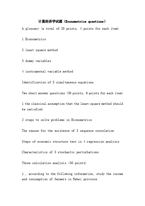
计量经济学试题(Econometrics questions)A glossary (a total of 20 points, 4 points for each item)1 Econometrics2 least square method3 dummy variables4 instrumental variable methodIdentification of 5 simultaneous equationsTwo short answer questions (30 points, 6 points for each item)1 the classical assumption that the least square method should be satisfied2 steps to solve problems in EconometricsThe reason for the existence of 3 sequence correlation Steps of economic structure test in 4 regression analysis Characteristics of 5 stochastic perturbationsThree calculation analysis (30 points)1., according to the following information, study the income and consumption of farmers in Hebei province.Requirements: (1) to establish regression model (list and calculation formula, test only for economic significance and goodness of fit test);(2) if the per capita net income of farmers in Hebei in 2008 is 3200 yuan, 2008 of the per capita living expenses of farmers in Hebei should be predicted.Particular yearItem 1994199519961997 1998199920002001 20022003Per capita net income of farmers (100 yuan) 111721232424252627 29Living expenses (100 yuan) 811141413131414151Four discussion questions (20 points)1 briefly describe the meaning, sources and consequences of heteroscedasticity, and write the test steps combined with the G-Q test method.Econometrics entry final exam questions B answerFirst, noun interpretation1 econometrics is the integration of mathematics, statistics and economic theory, combined with the theory and practice of economic behavior and phenomenon.2 least square method: the least square method for minimizing the sum of residuals of all observations is the least square method.3 dummy variables: there are some temporary factors in the study of economic life. Such as war, natural disasters, man-made disasters, these factors do not occur frequently in the economy, but with the same characteristics, these economists do not occur frequently, and temporary effect called virtual variables.4 instrumental variable method: instrumental variable method takes the predetermined variable as instrumental variable instead of the endogenous variable in structural equation as explanatory variable, in order to reduce the correlation between random item and explanatory variable.Identification of 5 simultaneous equations: a single equation that constitutes a simultaneous equation has only a statistical form in its simultaneous equations, and this equation is known to be identifiable, otherwise it is called non recognizable. If every equation in the simultaneous equation can be identified, this simultaneous equation is called identity, otherwise it is called non recognizable.Two, simple answer1 the classical assumption that the least square method should be satisfiedAnswer: (1) the mean of random items is zero;(2) random sequence non correlation and heteroscedasticity;(3) explanatory variables are non random, and if random, they are not related to random items;(4) there is no multicollinearity between explanatory variables.2 the steps of applying econometrics to solve economic problemsAnswer: 1) building models;2) estimation parameters;3) verification theory;4) use modelThe reason for the existence of 3 sequence correlationSequence correlation: that is, the random term U is related to other previous terms. It is called sequence correlation or autocorrelation.The cause of existence:First of all, with the continuous problem in economic life and time, namely the repetition time repeated, therefore, the explanatory variables associated with.Secondly, the error of model selection is established, which makes the explanatory variables relevant.Finally, when the model is established, the random term has autocorrelation, and the sequence has autocorrelation.The method of economic structure test in 4 regression analysisChow puts forward the following test method:Firstly, two samples were merged to form the sample of the number of observation value +, and the model (4.25) was regressed, and the regression equation was obtained:(4.28)The sum of squares of residuals is obtained, and the degree of freedom is + -k-1,Here K is the number of variables explained.Secondly, the use of two small sample given above, respectively (4.25) of the regression analysis, the regression equation respectively (4.26) and (4.27), calculated the sum of squared residuals, respectively, the degree of freedom for -k-1 and -k-1 respectively.Then, according to the sum of squares of residuals, the following statistic is constructed:~ F (k+1, + -2k-2) (4.29)Using statistical (4.29) test (4.26), (4.27) the significant similarities and differences, that is, test hypothesis: (j=0, 1,2,... K).Given the significant level (such as =0.05, =0.01), the F distribution table with the first degree of freedom as k+1 and the second degree of freedom as the + -2k-2 is obtained, and the critical value is obtained.If rejected, that (4.26), (4.27) there is a significant difference, the economic relations of the two or two samples reflect different, we say that the changes in the economic structure; on the contrary, we believe that the economic structure is relatively stable.Some properties of the 5 random perturbation term:1. the complex represented by many factors on the explanatory variable Y;2., the influence direction of Y should be different, there are positive and negative;3. as a secondary factor, the total average impact on Y may be zero;The effect of 4. on Y is non trending and stochastic.Three computational analysis1., according to the following information, study the income and consumption of farmers in Hebei province.Particular yearItem 1994199519961997 1998199920002001 20022003Per capita net income of farmers (100 yuan) 111721232424252627 29Living expenses (100 yuan) 811141413131414151According to economic theory, there is a correlation between farmers' living expenditure and their net income. The basic source of farmers' consumption expenditure lies in their net income, so the increase of per capita net income of farmers is the reason for the increase of their living expenses. In addition, farmers' living expenses are also affected by savings, psychological preferences and other factors, so the model is regression model.If Ct is the farmer's consumption expenditure, and Y is the net income per capita of farmers, the following regression model can be establishedCt=c+aYtDependent Variable: CTMethod: Least SquaresDate: 12/15/97 Time: 16:44Sample: 19942003Included observations: 10Variable Coefficient Std. Error t-Statistic Prob.YT 0.406238 0.046500 8.736250 0C 3.978409 1.080867 3.680755 0.0062R-squared 0.905126 Mean dependent var 13.20000Adjusted R-squared 0.893266 S.D. dependent var 2.250926 S.E. of regression 0.735380 Akaike info criterion 2.399998 Sum squared resid 4.326269 Schwarz criterion 2.460515Log likelihood -9.999988 F-statistic 76.32207Durbin-Watson stat 1.329130 Prob (F-statistic) 0.000023 The regression equation was Ct=3.9784+0.4062Yt(3.6801) (8.7363)Because T (a) =8.7363>T0.025 (8) =2.306F=76.3221>F0.05 (1,8) =5.32So the regression equation and its coefficients are significantR2=0.9051, which shows that the regression equation and the sample observation value have good goodness of fitFour topics1. answers:Meaning: for the random perturbation of the UI regression model, if the other assumption, the second assumption is not established, that is to say in the variance of random UI different observation value is not equal to a constant, Var (UI) = constant (i=1, 2,... (n), or Var (U) Var (U) (I J), then we call the random perturbation term UI has heteroscedasticity.Source: 1. model omitted economic variables, the measurement error of 2.The consequence of heteroscedasticity: the 1. parameter estimator is still linear unbiased, but not valid. 2. test failure based on t distribution and F distribution. The variance of 3. estimator increases, and the prediction accuracy decreases.Inspection: Inspection (Goldfeld - Quart Goldfield - Quandt G - Q test) test in 1965 by S.M.Goldfeld and R.E.Quandt proposed. This test method is applicable to large samples, usually require the capacity of n should be 30 or the number of observations is to estimate the parameters of more than 2 times(i.e., sample size is much larger than the N model included explanatory variables two times large numbers above). To test heteroscedasticity should meet the following conditions: first, using the method of random perturbation UI obey the normal distribution, and the variance of UI increased with a certain explanatory variables; second, random perturbation UI no serial correlation, namely E (uiuj) =0 (I J). The test method is mainly F test.The test hypothesis H0: UI is equal variance, and the alternative assumption is that H1: UI is heteroscedastic, and the specific steps of G - Q test are as follows:1. will explain the observed value of the variable Xi in absolute ascending order, be interpreted correspond to the variables of Xi Yi.2. the Xi are arranged in C values by deleting the centre of the remaining N-C observations is divided into two sub samples of the same capacity, the capacity of each sub sample respectively, a sub sample which is the larger part of the corresponding observation value, the other is a relatively small part of the observed value. It should be noted that the determination of the C value is not arbitrary, and it is determined by experiments by Goldfeld and Quandt. For the sample size when n is greater than 30, the number of C for the entire sample number 1/4 by deleting observations (e.g., sample size is 48, c=, n=12, removal of the observation value is 12, then the two sub sample volume respectively =18).3. the least squares method is used to calculate the regressionequation of the two sub samples, and then the corresponding residual sum of squares is calculated respectively. The sum of squares of residuals is the sum of the residuals of the sub samples with larger sample value, and their degree of freedom is -k, where k is the number of explanatory variables in the econometric model.4. establish statistics:F= can prove that F=RSS2/RSS1 ~ F (), that is, it follows the F distribution of degrees of freedom respectively. Obviously, if the two sub sample variance is equal, the value of F is close to 1, show that UI has equal variance; if the variance is not equal, according to the pre condition of RSS2 is greater than RSS1, F-measure should be greater than 1, then UI has heteroscedasticity, so we can use the F test to verify whether UI has heteroscedasticity of. That is, for the given significance level, the F distribution table is obtained corresponding critical value, if F>, reject H0, accept H1, that is, UI has heteroscedasticity; if F<, then accept H0, UI has equal variance.。
计量经济学简介

Function Y=f(x) ? Random Variables Correlation between y and x? Not causality
since w may be correlated with other factors that also affect y.
6
Ceteris Paribus Analysis
10
Example 1: Effects of Fertilizer on Soybean Yield
Intuition tells us that more fertilizer should lead to higher yields. Experiment? In the simplest case, this implies an equation like:
计量经济学
计量经济学是以一定的经济理论和统计资料为基础, 运用数学、统计学方法与电脑技术,以建立经济计量 模型为主要手段,定量分析具有随机性特性的经济变 量关系,主要内容包括理论计量经济学和应用计量经 济学。理论经济计量学主要研究如何运用、改造和发 展数理统计的方法,使之成为随机经济关系测定的特 殊方法。应用计量经济学是在一定的经济理论的指导 下,以反映事实的统计数据为依据,用经济计量方法 研究经济数学模型的实用化或探索实证经济规律。 计量经济学广泛采用计算机组织教学,着重培养学生 定量地分析问题、解决问题的能力。
Deciding on the list of proper controls is not
always straightforward, and using different controls can lead to different conclusions about a causal relationship between y and w.
70年代后计量经济学发展简史

70年代后计量经济学发展简史在上世纪70年代以前,计量经济学研究经历了从简单到复杂、从单一方程到联立方程的进化过程。
进入70年代,西方国家致力于更大规模的宏观计量经济模型研究。
为了理解、预测和控制经济运行过程,计量经济学从着眼于研究适合国内的计量经济模型发展到着眼于国际的大型计量经济模型,以便研究国际经济波动的影响和国际经济发展战略可能引起的各种后果,为制定和评价长期的经济政策服务。
70年代是联立方程模型发展最辉煌的时期。
最著名的联立方程模型是“连接计划”(Link Project),截至1987年,该模型已包括78个国家2万个方程。
这一时期最有代表性的计量经济学家是L.Klein教授,他于1980年获诺贝尔经济学奖。
但是,后来人们发现有的时候联立方程模型的预测能力并不像想象的那样强,模型结构也不稳定。
于是,人们开始寻找它的原因:首先,人们想到的是计量经济学的基本假设,其核心假定是“经济时间序列是平稳的”(注:平稳序列的典型特征是,它的一阶矩和二阶矩都是常数,不随时间而变)。
70年代以前的建模技术都是以“经济时间序列平稳”这一假定为前提的。
然而,70年代后各国的经济结构有了很大变化(石油危机、汇率波动、滞涨等),经济变量出现了非平稳特征。
其次,人们还发现了计量经济模型的“伪回归”问题。
由于经济时间序列的非平稳性和“伪回归”问题直接影响经济计量模型参数估计的准确性,人们开始对计量经济学方法论的缺陷提出质疑。
方法论(Methodology)是指处理问题和从事活动的方式,它构成了我们完成一项任务的一般途径,提供了组织、计划、设计和实施研究的基本原则。
几件主要的事情,促成了协整(协积)分析方法论的形成和发展完善:1974年,Granger-Newbold首先提出“虚假回归”问题。
Granger指出,经济变量间存在可测的因果关系的必要条件应包括,模型参数对于输入变量所含干扰信号具有抗变性。
1967年,Box-Jenkins出版《时间序列分析、预测与控制》一书。
ch16 Simultaneous Equations 《计量经济学导论》课件
of a2, the slope of the demand curve We cannot estimate a1, the slope of the
supply curve
Economics 20 - Prof. Anderson
7Байду номын сангаас
The General SEM
Suppose you want to estimate the structural
equation: y1 = a1y2 + b1z1 + u1 where, y2 = a2y1 + b2z2 + u2 Thus, y2 = a2(a1y2 + b1z1 + u1) + b2z2 + u2 So, (1 – a2a1)y2 = a2 b1z1 + b2z2 + a2 u1 +
a1 is biased – call it simultaneity bias
The sign of the bias is complicated, but can use the simple regression as a rule of thumb
In the simple regression case, the bias is the
Economics 20 - Prof. Anderson
2
Supply and Demand Example
Start with an equation you’d like to estimate, say a labor supply function
计量经济学导论-ch16
© 2013 Cengage Learning. All Rights Reserved. May not be scanned, copied or duplicated, or posted to a publicly accessible website, in whole or in part.
© 2013 Cengage Learning. All Rights Reserved. May not be scanned, copied or duplicated, or posted to a publicly accessible website, in whole or in part.
Rank condition The first equation is identified if, and only if, the second equation contains at least one exogenous variable that is excluded from the first eq.
© 2013 Cengage Learning. All Rights Reserved. May not be scanned, copied or duplicated, or posted to a publicly accessible website, in whole or in part.
simultaneous three-equation model
simultaneous three-equation model1. 引言1.1 概述在经济学和社会科学研究中,同时考虑多个相关方程的模型被广泛应用。
这些模型被称为"simultaneous three-equation models",因为它们包含三个相互关联的方程。
这些方程通常代表着不同的经济变量之间的关系,通过分析这些关系可以更好地理解经济系统的运作机制。
1.2 文章结构本文将对simultaneous three-equation model进行详细的探讨和分析。
首先,我们将介绍该模型的理论背景,包括概述、模型假设以及应用领域。
接下来,我们将阐述模型的建立过程和参数估计方法,并介绍模型选择准则和诊断检验。
然后,我们将展示实证分析结果,并对其进行解释和讨论。
最后,我们将总结主要研究发现并展望存在的问题与改进研究方向。
1.3 目的本文旨在提供一个全面而深入的介绍simultaneous three-equation model,并通过实证分析来展示其在经济学研究中的应用价值。
我们希望通过对该模型的探讨和分析,能够增加读者对经济系统运作机制的理解,并为相关领域的研究和政策制定提供有益的参考。
同时,我们也将指出该模型存在的问题,并展望未来改进研究的方向。
2. 理论背景2.1 三方程模型概述在经济学和社会科学领域,三方程模型是一种常用的统计分析方法。
该模型通过建立三个联立方程来描述多个变量之间的关系和相互作用。
这些方程通常代表着不同变量之间的因果关系,可以揭示出导致某一现象或结果的因素。
三方程模型通常包括三个主要成分:自变量、因变量和错误项。
自变量是研究者选定的与因变量有关的解释变量,它们对因变量产生直接或间接影响。
因变量是研究者希望解释或预测的目标变量。
错误项则代表了未被观察到或遗漏的其他影响因素,即未能被自变量完全解释并捕捉到的部分。
2.2 模型假设为了建立一个有效的三方程模型,需要满足一些基本假设。
第八章-联立方程模型
由于在求解模型时,通常是需要联立地解出所 有内生变量的值,因而称为联立方程模型。
单方程模型中,内生变量就是因变量,外生变 量是解释变量(滞后内生变量除外)。
3.前定变量(predetermined variable)
R , UN。
不难看出,在上述两例中,方程的左端都
是内生变量。联立方程模型中每个方程的左端 为不同内生变量原型的写法,称为方程的正规 化。
四、模型的结构式和简化式
1.结构式(Structural form)
联立方程模型的结构式是依据经济理论设定模型 时所采取的形式。其中的方程称为结构方程,一个 结构方程反映一个基本的经济关系,即对经济理论 的一种阐述。结构方程的参数称为结构参数。
让我们再看一个例子,由菲利普斯工资方程和价格方程组成 的模型:
Wt 0 1UNt 2Pt u1t (4)
Pt 0 1Wt 2Rt 3Mt u2t (5)
其中 W 货币工资变动, UN = 失业率
P =价格变动,
R = 资金成本变动
M =进口原料费用变动
在此模型中,内生变量是:W,P, 外生变量是:M ,
二、 行为方程和恒等式
1.行为方程(behavioural equation)
凯恩斯收入决定模型中的消费函数是一个行为方 程,它描述的是消费者的行为,即在给定收入的情 况下平均而言,消费者的行为是怎样的。除了描述 消费者行为的方程外,还有描述生产者、投资者及 其它经济参与行为的方程,他们都是行为方程。
Qt = 0 1Pt 2 Yt v t
其中: 0
0 0
1
1
- 1、下载文档前请自行甄别文档内容的完整性,平台不提供额外的编辑、内容补充、找答案等附加服务。
- 2、"仅部分预览"的文档,不可在线预览部分如存在完整性等问题,可反馈申请退款(可完整预览的文档不适用该条件!)。
- 3、如文档侵犯您的权益,请联系客服反馈,我们会尽快为您处理(人工客服工作时间:9:00-18:30)。
Random errors are added to the supply and demand equations to account for unobserved effects, models, , as in the single g equation q , but this time as we have 2 equations we need to make an assumption about the covariance between them
Based we expect B d on economic i theory th t the th supply l curve to t be b positively sloped 1>0, the demand curve to be negatively sloped 1<0. Quantity demanded (Q) is a function of price (P) and income (X), income is determined outside this system and is said to be exogenous Quantity supplied (Q) is only a function of price (P)
In a supply and demand model, the market equilibrium occurs at the intersection of the supply and demand curves An econometric model that explains market price and quantity should consist of two equations, one for supply and the other for demand. The supply and demand equations work together, together to find the equilibrium we need them both
Principles of Econometrics, 3rd Edition
Suggested exercises
Slide 11-2
1
11/3/2010
Principles of Econometrics, 3rd Edition
We are now going to study models that are jointly
Slide11-10
Principles of Econometrics, 3rd Edition
5
11/3/2010
This picture recognizes that supply (Q) and demand (Q) are jointly determined, with joint dependence on Price (P) Because of this dependence we cant reliably estimate the model for P or Q using Slide11-11 OLS
7
11/3/2010
The reduced form equations helps us understand the SEM To find the reduced form we use the equilibrium condition and equate the two quantities and the solve for P
Principles of Econometrics, 3rd Edition
3
11/3/201011.1)
Supply: Q 1P es
(11.2)
Principles of Econometrics, 3rd Edition
To solve for Q, we can substitute the value for P into either the demand or supply equations, we use the supply eqn as its simpler
Q 1P es 2 e e 1 X d s es 1 1 1 1 1 2 e 1es X 1 d 1 1 1 1 2 X v2
1 P es 1 P 2 X ed
P
2 e e X d s 1 1 1 1
(11.4)
1 X v1
Note that Price (P) is a –ve function of es 1<0, 1>0 Slide11-15
2 E (ed ) 0, var(ed ) d
E (es ) 0, var(es ) 2 s cov(ed , es ) ds
(11.3)
Principles of Econometrics, 3rd Edition
Slide11-8
4
11/3/2010
In this system price (P) and quantity (Q) are simultaneously l l or jointly l d determined, d as their h values l are determined within the system In SEM its incorrect to simply assume that the endogenous variables are those that just appear on the LHS of at least one equation We could just have easily written the supply equation with ith P on the th LHS and d everything thi else l on the th RHS A variable is endogenous if it is jointly determined Endogenous variables Qs , Qd , P In this system Income (X) is an exogeneous variable
In this representation there is no equilibriating mechanism, that relates Qs to Qd If supply (Q) and demand (Q) had no relationship to each other (e.g. inelastic supply) and could be observed, then least squares could be used to estimate these relationships
determined by two or more economic relations These models are called simultaneous equations as there are two or more dependent variables that are jointly determined In economics, the supply and demand model is an example of a simultaneous equation model Price and the quantity demanded are determined by the interaction of two equations, q , one for supply pp y and the other for demand We will explain why the least squares estimation procedure is not appropriate in these situations
For a given Income (X), we only observe the equilibrium
6
11/3/2010
Principles of Econometrics, 3rd Edition
The equations derived from economic theory (such as in the supply and demand model) are known as the structural equations We cant use OLS to directly estimate the structural model parameters due to simultaneous equations bias Simultaneous equations bias arises because the error terms affect both P and Q suggesting a correlation between the endogenous variables on the RHS and th error terms the t on the th RHS, RHS we will ill show h this thi later l t However we can solve the structural equations and write each endogenous variable solely as a function of the predetermined variables, giving the reduced‐ form equations