自动控制原理课件拉氏变换.ppt
《拉氏变换详解》课件

积分性质
积分性质
若 $f(t)$ 的拉普拉斯变换为 $F(s)$, 则 $int_{0}^{infty} f(t) dt$ 的拉普拉 斯变换为 $- frac{1}{s} F(s)$。
应用
积分性质在求解初值问题和极值问题 时非常有用,可以方便地得到原函数 的表达式。
微分性质
微分性质
若 $f(t)$ 的拉普拉斯变换为 $F(s)$,则 $f^{(n)}(t)$ 的拉普拉斯变换为 $s^{n} F(s) - s^{n-1} f(0-) - s^{n-2} f'(0-) - ldots - f^{(n-1)}(0-)$。
卷积定理
总结词
卷积定理是拉普拉斯变换的一个重要特性, 它描述了函数与其导数之间的卷积关系。
详细描述
卷积定理表明,对于任意实数t,如果函数 f(t)与其导数f'(t)的拉普拉斯变换都存在,则 它们之间的卷积结果等于零。这个定理在信 号处理、控制系统等领域有着广泛的应用, 可以帮助我们更好地理解和分析函数的性质
,再通过反变换得到 (y(t))。
控制系统的稳定性分析
总结词
通过拉普拉斯变换,可以分析控制系统的稳定性,为系 统设计和优化提供依据。
详细描述
对于线性时不变控制系统,通过拉普拉斯变换,可以将 其转化为传递函数的形式。根据传递函数的极点和零点 分布,可以判断系统的稳定性。如果所有极点都在复平 面的左半部分,则系统是稳定的。如果极点在右半部分 或等于零,则系统是不稳定的。此外,系统的动态性能 也可以通过传递函数的极点和零点分布进行分析和优化 。
03
动态行为。
2023
PART 02
拉普拉斯变换的应用
REPORTING
在微分方程中的应用
自动控制原理(拉氏变换)
置信号。
精品PPT
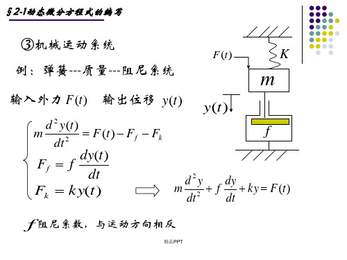
§3-1控制系统的暂态响应分析
② 斜坡(匀速)输入
xr(t)
0 t0
A
xr
(t)
At
t0
0
t
相当于随动系统加入一按恒速变化的位置信号, 该恒速度为A。
精品PPT
§3-1控制系统的暂态响应分析
③抛物线(匀加速)输入
xr(t)
0 t0
xr
(t
)
At2
t0
0
t
相当于随动系统加入一按恒加速度变化的位置 信号,该恒加速度为A。
tu(t)
1 s2
精品PPT
例5正弦函数
精品PPT
周期函数的拉普拉斯变换
可以证明:若 f (t)是周期为T 的周期函数,即
f (t T ) f (t) (t 0)
当 f (t)在一个周期上连续或分段连续时,则有
1
ℒ f (t) 1 es T
T f (t)es tdt
0
这是求周期函数拉氏变换公式
精品PPT
§2-2非线性数学模型的线性化
2. 数学描述 设系统的输入为x(t),输出为y(t), 且满足y(t)=f(x),其中f(x)为非线性函数。 设t=t0时,x=x0,y=y0为系统的稳定工作点
(x0,y0), y(t)
y(t) f (x)
y0
x0
精品PPT
x(t)
§2-2非线性数学模型的线性化
k R.
解
ℒ
f (t)
ektest dt e(sk )t dt 1
0
0
sk
ekt 1
sk
Res k
例4
求单位斜坡函数
二章2拉氏变换ppt课件

五、拉氏变换求解线性微分方程
➢将微分方程通过拉氏变换变为 s 的代数方程; ➢解代数方程,得到有关变量的拉氏变换表达式; ➢应用拉氏反变换,得到微分方程的时域解。
A1 A2 A3 S S2 S3
A1
S S
1
2S
3
S
S 0
1 6
A2
S S
1
2S
3 S
2
S 2
1 2
A3
S S
1
2S
3 S
3
S 3
1 3
1
Y(S) 6
1 2
1 3
S S2 S3
yt 1 1 e2t 1 e3t
62 3
1 e2t 1 e3t
2
3
1
S 0.5
0.57 0.866
S S 0.52 0.8662 S 0.52 0.8662
f t 1 e0.5t cos 0.866 t 0.57e0.5t sin 0.866 t
3、A(S)=0有重极点
设A(S)=0有r个重极点,将F(S)展开成下列形式:
FS
S
A01
P0 r
1 !
例3:求
F
S
S
S 3
22 S
1
的反变换
将F(S)展开成下列形式:
FS
S
A01
22
A02
S 2
A3
S 1
A01
S
S 3
22 S
1 S
22
S 2
1
A02
d
ds
S
S 3
22 S
1 S
22
S
2
2
自动控制原理课件-拉氏变换专讲

a3 an a1s a2 F ( s) s p1 s p2 s p3 s pn
1
a1s a2 s p
F ( s )s p1 s p2 s p
1
根据上述方程,令实部=实部,虚部= 虚部,可解出a1,a2
s 1 例: 求 F ( s ) 2 s s s 1 的部分分式 a3 a1 s a2 解: F ( s ) 2 s s 1 s
用拉氏变换法求解微分方程(2)
1 A a b
1 B a b
1 1 1 ba ba s a s b s a sb
用拉氏变换法求解微分方程(2)
留数法(适用于复杂函数)
s z1 s zm B( s ) 设 F ( s) A( s) s p1 s pn
a1 F (s)s 1
3 s 1
s 2s 3
2
s 1
2
用拉氏变换法求解微分方程(6)
d F ( s )s 1 a2 ds
2
3
s 1
2 s 2 s 1 0
3
1 d F ( s )s 1 a3 2 3 1! ds
2
令
A B C Y ( s) s s2 s3
2 1
0.866a1 a2 0.866
2
0.5
用拉氏变换法求解微分方程(5)
化简: a1 a2 1 求解得:
a1 a2 1
a2 0
a1 1
s 1 a3 s 1 2 s s s 1 s 0
拉氏变换详解ppt课件
0
a
令t / a , 则原式 f ( )e
0
sa
ad aF (as)
9
(8)卷积定理 两个原函数的卷积的拉氏变换等于两个象函 数的乘积。 t 即 L[ f (t ) f ( )d ] F ( s) Nhomakorabea ( s)
0 1 2 1 2
证明: L[ f1 (t ) f 2 ( )d ] [ f1 (t ) f 2 ( )d ]e dt
原函数之和的拉氏变换等于各原函数的拉 氏变换之和。 (2)微分性质 若 L[ f (t )] F ( s) ,则有 L[ f (t )] sF (s) f (0) f(0)为原函数f(t) 在t=0时的初始值。
3
证:根据拉氏变换的定义有
L[ f (t )] f (t )e dt s f (t )e dt f (t )e
st st 0 0
st 0
sF ( s) f (0)
原函数二阶导数的拉氏变换
L[ f (t )] sL[ f (t )] f (0) s[ sF ( s) f (0)] f (0) s 2 F ( s) sf (0) f (0)
14
2. 拉式反变换——部分分式展开式的求法
M (s) b0 s b1s bm1s bm F ( s) n (m n) n 1 D(s) s a1s an1s an
m
m1
(1)情况一:F(s) 有不同极点,这时,F(s) 总能展开成如下简单的部分分式之和
f (t ) L [ F ( s)] t 1 e
工程控制理论-拉普拉斯变换ppt

L
df (t) dt
sF (s)
f
(0)
证明:
L
df (t) dt
df (t) estdt 0 dt
estdf (t)
0
est f (t) s f (t)estdt sF (s) f (0)
0
0
同理,对于二阶导数的拉普拉斯变换:
L
d2 f dt
(t)
2
s2F
(s)
t
s0
2.2.4 拉普拉斯变换的基本性质
(6) 初值定理
若: L f (t) F(s)
则:
lim f (t) lim sF (s)
t 0
s
证明:根据拉普拉斯变换的微分定理,有
lim
s
0
df (t dt
拉普拉斯变换简表 (续3)
序号
原函数 f(t) (t >0)
象函数 F(s) = L[f(t)]
13
1 a
(1-e -at )
1 s(s+a)
14
1
b-a
(e -at -e -bt )
1 (s+a) (s+b)
15
1
b-a
(be
-bt
-ae
–at
)
s (s+a) (s+b)
16
sin(t + )
cos + s sin s2+2
L eat eatestdt e(sa)tdt 1
0
0
sa
2.2.3 典型时间函数的拉普拉斯变换
(5) 正弦信号函数
正弦信号函数定义:
两 e jt cost jsin t
自动控制原理拉氏变换
s
δ(t )
d [
ε(t )]
S
1
1
dt
S
df (t) dt
sF (s)
f
(0 )
3.积分性质
重点!
设: [ f (t)] F(s)
则:
t
1
[ 0
f
(t)dt]
F(s) s
证:令
t
[ 0
f
(t)dt]
φ(s)
[ f (t)]
dt
F(s) K - Ke-t
K K Ka s s a s(s a)
2. 微分性质
若: f (t) F(S) udv uv vdu
则
df ( t dt
)
sF ( s )
f
(0 )
重点!
证:
df ( t dt
例13-8
求:F(s)
s2
1 (s 1)3
的原函数f
(t)
解
F(s)
K22 s
K21 s2
K13 (s 1)
K12 (s 1)2
K11 (s 1)3
以(s+1)3乘以F(s)
(s
1)3
F (s)
1 s2
1
K11 s2 s1 1
K12
d ds
1 s2
s1
注 f (t t0) 0 当 t t0
证:
f(t - t0 )
0
f (t t0 )estdt
自动控制原理拉氏变换
3.拉氏变换的基本定理 ¾线性定理
若函数分别有其拉氏变换:
f1(t) ⇒ F1(s) f2 (t) ⇒ F2 (s) 则
L[af1(t) + bf2 (t)] = aF1 (s) + bF2 (s)
¾延迟定理
若 f (t) ⇒ F (s)
则
L[ f (t −τ )] = e−τs F (s)来自根据拉氏变换的 基本定理
部
分
分母全部为单根
分
式
法
分母有重根
¾A(s)=0 全部为单根
ai 为F (s) 对应于极点 si 的留数。
例:已知 解:
求 F (s) 拉氏反变换。
¾A (s) =0 有重根
。。。。。。
例:求
解:
的拉氏反变换 f (t) 。
例:已知
解:
,试求其 f (t)
6. 应用拉氏变换解微分方程
¾ 方程两边作拉氏变换 ¾代入初始条件和输入信号 ¾写出输出量的拉氏变换
¾作拉氏反变换求出系统输出的时间解
例 RC滤波电路如图所示,输入电压信号Ui(t)=5V,
电容的初始电压 Uc(0) 分别为 0V 和1V 时,分
别求时间解Uc(t)。
解:
¾Uc(0)=0V 时 ¾Uc(0)=1V 时
¾终值定理
若 f (t) ⇒ F (s) 且 f (∞) 存在,则
¾卷积定理
若 f1(t) ⇒ F1(s) f2 (t) ⇒ F2 (s) 则
求 ?
4. 拉氏变换的优点:
¾简化函数
¾简化运算
5. 拉氏反变换
拉氏变换: 已知 f ( t ) → 求 F (s) 拉式反变换: 已知 F (s) → 求 f ( t )
l自动控制原理 第三讲 拉氏变换
Lecture3-Laplace TransformsK.J.ÅströmReview of control system analysis1.The Basic Feedback Loopplace T ransforms3.Analysis of Feedback Loops4.Qualitative Understanding of Signals and Systems5.SummaryTheme:Streamline manipulation of equations and block diagrams.Construction of a Block DiagramThe block diagram gives an overview.T o draw a block diagram:•Understand how the system works.•Identify the major components and the relevant signals.•Key questions:Where is the essential dynamics?What are appropriate abstractions?•Describe the dynamics of the blocks in terms of standard models.dt n+a1dn−1ydt n−1+...+b n u is characterized by two polynomialsA(s)=s n+a1s n−1+a2s n−2+...+a n−1s+a nB(s)=b1s n−1+b2s n−2+...+b n−1s+b n•The roots of A(s)are called poles of the system.•The roots of B(s)are called zeros of the system.•The transfer function of the system is G(s)=B(s)Linear Time Invariant Systems(LTI)d n ydt n−1+...+a n y=b1dn−1uInterpretation of the Impulse Responsey(t)=nk=1C k−1(t)eαk t+t(t−τ)u(τ)dτLet the system be initially at rest,i.e.C k=0and let the inputbe an impulse at time0.The output is theny(t)= (t)If the input is a unit step the output(the step response)isy(t)=t(t−τ)dτ=t(τ)dτExperimental determination of step and impulse responses.Recall Cruise ControlProcess modeldvdt2+(0.02+k)dedtThe mathematical tool of Laplace transforms is ideally suitedfor these type of calculations.An essential part of the languageof control.place TransformsConsider a function f defined on 0≤t <∞and a real number σ>0.Assume that f grows slower than e σt for large t .The Laplace transform F =L f of f is defined asL f =F (s )= ∞e −stf (t )dtExample 1:f (t )=1,F (s )=∞e −st dt =−1sExample 2:f (t )=e −at ,F (s )=∞e −(s +a )t dt =−1s +adt=∞e −stf (t )dt =e −st f (t )∞0+s∞e −stf (t )dt =−f (0)+s L fs)dv =f (0)Final value theoremlim s →0sF (s )=lim s →0∞0se −st f (t )dt =lims →0∞e −vf (vPropertiesLinearity:L (a f +b )=a L f +b L Differentiation:L dfs L fTime shift:L f (t −T )=e −sTL fTime stretch:L f (at )=1a ),a >0.Convolution:L t0f (t −τ) (τ)d τ=F (s )G (s )Final value Theorem †:lim s →0sF (s )=lim t →∞f (t )Initial value Theorem †:lim s →∞sF (s )=lim t →0f (t )•†:V alid only if limits exist!A (s )=B (s )s −α1+C 2s −αnC k =lim s →αk(s −αk )F (s )=B (αk )The time function corresponding to the transform isf (t )=C 1e α1t +C 2e α2t +...+C n e αn tParameters αk give shape and numbers C k give magnitudes.Notice that αk may be complex numbers.With multiple roots the constants C k are instead polynomials.Manipulating LTI Systems The differentiation property L dfCruise ControlProcess model:dvsE(s)Pure algebra gives relation between Laplace transforms of slopeΘreference V r and E by eliminating V and Us(s+0.02)+ks+k iE(s)=10sΘ(s)+s(s+0.02)V r(s)2+2ω0s+ω20Θ(s)=10θ0ω0te−ω0tω0te−ω0tThe largest error e max=10θ0e−1occurs for t=1/ωparegraph belowθ0=0.04ζ=1,ω0=0.05(dotted),ω0=0.1Discussion•What do we mean by a solution to a problem?•A historical perspectiveClosed form expressions,tables,curves •The role of computers•The necessity of insight and understanding•The need to check results•What properties can wefind easily using“back of an envelope”calculation.•A perspective on use of Laplace transforms in control engineering•A more general(biased personal)perspective.T echnology changes fast but engineering education changes slowly.U(s)=L yCar Model in Cruise Control Process modeldvU(s)=1U(s)=−10Transfer Function of PID ControllerThe error e is the input and the control signal u is the outputu=ke+k ite(τ))dτ+k ddeE(s)=k+k iTransfer Function of CarA simple model of a car on a horizontal road tells how its position y depends on the throttle.Let the mass be m and assume that the propelling force is proportional to the throttle wefindmd2yU(s)=kTransfer Function of Time DelayConsider a system where the output y is the input u delayed Ttime units.The input output relation isy(t)=u(t−T)and the transfer function isG(s)=Y(s)Transfer Function of Standard Model Consider the systemd n ydt n−1+...+a n y=b1dn−1us n+a1s n−1+a2s n−2+...+a n−1s+a nSolutionIntroduce Laplace transforms and transfer functions.We haveE =R − N +P (D +CE )Solving for E givesE =11+PCN −P5.Qualitative Understanding of Signals andSystemsTime responses can in principle be computed.T ables of Laplace transforms is a help but the work is quite tedious.Time responses are easy to compute using different types of software.•It is a good rule to always make order of magnitude calculations to make sure that results are reasonable whenever you use software.•Much insight can be obtained form very simple calcula-tions (series expansions and factorization).•Some results will be presented.•It will be discussed more in future lecturesA (s )=B (s )s −α1+C 2s −αnC k =lim s →αk(s −αk )F (s )=B (αk )Parameters αk (roots of A (s ))are easy to compute.The signal y (t )has the formy (t )=C 1e α1t +C 2e α2t +...+C n e αn tParameters αk give shape and C k give magnitudes.A (s )=s +5Example...For small s the Laplace transform is Y(s) 2.5/s,which implies that for large t the time function is y(t) 2.5.For larges we have Y(s) 1/s2.This means that for small t the time function isC(s)=s+5Insight from Transfer Functions•Derive transfer function G(s)=B(s)Insight from Transfer Functions•Make a series expansion of G(s)for small s(low fre-quency behavior,large t)G(s)=c−1s+c−2s k+...If c0=0like a static gain.If c−1=0and c−1=0like an integrator.If c−1=c−2=...=c−k+1=0and c k=0like k integrators.ExamplesE XAMPLE 1—PID CONTROLLERThe PID controller has the transfer functionG (s )=k +k is+k +k d sThis is already in series expansion form.For slow signals(small s )it behaves like an integrator and for fast signals (large s )it behaves like a differentiator.E XAMPLE 2—PID CONTROLLER WITHD ERIVATIVEF ILTERG (s )=k 1+11+s T d /NBehaves like a static gain k (1+N )for fast signals (large s ).。
拉式变换课件
0
式中,s为复数变量;f t 为原函数;F s为象函数。
Page 4
拉氏变换的定义式:
记做
f (t) LT F (s) f (t)est dt 0
L [ f (t) ]= F (s) 或 f (t) LT F (s)
df (t) dt
est
f (t)
0
0
(s)e
st
f (t)dt
sF (s)
f (0 )
得证。
?
Page 23
uv'dx uv vu'dx
3.1.2 拉氏变换的性质
当 f(0)=f ’(0)=…f(n-1)(0)=0,则有:
L
2 s j0 s j0 s2 02
Page 20
பைடு நூலகம்
sin 0t
1 2j
(e j0t
e
) j0t
例:
L[sin 0t ]
1 2j
L[e
] j0t
1 2j
L[e
] j0t
1 2j
( s
1
j0
s
1
j0
)
0 s2 02
Page 21
3.1.2 拉氏变换的性质
(二)、 时域微分(differentiation)的拉氏变换
若L[ f (t)] F(s)
L
df (t dt
)
sF (s)
f
(0)
证明