HARP软件说明书之CHARM3D
MA3D中文说明书

GrandMA 3D中文说明书内容1引言52系统要求3安装63.1奶奶办公桌或奶奶onPC版本3.2的IP 73.3连接奶奶办公桌3.4 1姥姥或奶奶2模式4数据94.1主/从94.2坐标系统5个快速启动6计划表面6.1菜单栏6.2工具栏6.3(第一阶段视图,三维对象视图)主要的Windows6.3.1第一阶段检视6.3.2鼠标+键盘操作6.3.3安排(对齐对象)的对象6.3.4复制(复制的三维物体)6.3.5三维对象6.4资产(信息窗)6.5属性6.6媒体数据库6.7材料6.8移动Pathes6.9会议6.10状态栏7灯具类型8三维建模和导入8.1三维模型8.2参数8.2.1轴8.2.2旋转轴8.2.3线性轴8.2.4束光.8.3自动导入8.4分配模型夹具类型8.5三维建模清单8.6创建一个三维模型9视频创建10常见问题11个键盘快捷键12指数马照明科技有限公司Dachdeckerstr。
16 D - 97297Waldbüttelbrunn1引言:奶奶3D是一个独特的新的用户界面,三维可视化创建利用与奶奶产品范围结合的阶段布局。
系列I和系列第二站的支持。
该软件被设计成一个灯光设计师的预编程工具。
它简化了创建显示,以节省时间和金钱的过程。
奶奶3D包括一个基本图形元素库。
使用多个窗口前/侧/顶视图可以在同一时间打开和更新。
所有的舞台元素被定位在X / Y / Z方向,也可能是周围的各种轴旋转。
习俗这些元素的表面纹理,可以导入位图格式,或可能选择从一个图书馆。
灯笼,灯具或移动灯的设置,可以简单地检索到的奶奶控制台或电子转帐的奶奶onPC每放映文件。
有没有需要设置的DMX 线,DMX地址或单个装置的操作模式,因为这些细节,都已经预先调整中的奶奶。
当切换到3D渲染模式,奶奶3D软件变得极其强大的可视化实时渲染设施。
所有绘图元素,装置及灯笼与表面纹理,作为一种虚拟现实。
的所有功能。
安装路灯远程控制连接的奶奶办公桌和onPC逼真的动作,颜色和图像显示。
H-rior软件操作手册
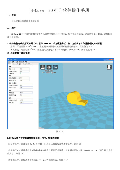
H-Cura3D打印软件操作手册一、安装软件下载安装请联系客服人员二、操作H-Cura3D打印软件自身的参数可以满足多数用户打印要求;如有更高的需求,则需调整部分数据,请仔细阅读下面说明。
1.软件安装完成后界面如图(1),拉取Test.stl于方格置物区,左上方会显示打印所需时间及耗材量层高:可变范围0.06~0.4mm,数值越小表面越细腻但同时花费时间越长,默认值为0.2填充密度:可变范围0~100,数值越大强度越大花费时间越长,默认为20%,图中设置为40%※其余参数不建议修改图(1)2.H-Cura软件中含有调整模型角度,尺寸,镜像的功能①调整角度:通过拉伸X,Y,Z三轴上对应显示的弧线调整所需角度,如图(2)②调整尺寸:通过修改比例参数或者直接修改所需尺寸调整,若单侧变形则点选Uniform scale“锁”标志后修改尺寸,如图(3)③镜像文件:镜像选项中提供X,Y,Z三种镜像格式,如图(4)图(2)图(3)图(4)3.预览打印时的观察方式H-Cura软件中提供5种观察方式,这里介绍常用的正常模式(Normal)和分层打印轨迹预览(Layers);①正常模式(Normal):模型导入置物框时均为这种模式,也只有在这种模式下才可以调整角度大小,如图(5)②分层打印轨迹预览(Layers):模拟打印路线,可以看到每一次的打印情况,通过这个模式可以调整模型的最佳打印角度,如图(6)4.鼠标的配合使用①左键选定模型移动,右键旋转方格置物框,滚轴放大/缩小方格置物框②选定模型后右键菜单如图(7),有些大型模型需要分开打印进行组装,可以通过拆分成零件实现。
图(5)图(6)图(7)5.软件打印①将模型拉取至方格置物框内,调整好所需参数和打印角度②将打印机连接电脑后,选择开始打印,如图(8)③坦诚窗口显示为目前喷头温度点击打印,如图(9)首次连接电脑时,系统会自动安装打印机驱动,若用USB连接电脑后没有弹出驱动安装成功的提示,检查电脑设备管理器→端口是否有COM X端口。
日本LookStailorX3D打板软件说明书_1
介绍LookStailorXLookStailorX 是一个发展从一个3D garment.It 2D 模式的三维服装设计系统为图案在服装业提供一种创新的方法。
LookStailorX 是由三个模块,其中包括人体模块、服装模块和模式模块组成。
人体模块用于创建一个机构负责服装建模、服装模块用于模型为身体使用一种基于草绘的方法,通过更改它的等高线修改服装形状的三维服装和模式模块用于绘制线条设计研发2D 模式。
***************************************系统模块当LookStailorX启动,将显示第一个模块是模特模块。
对操作顺序是从模特模块服装模块,然后格局模块。
根据工作需要做,可以选择任何模块。
点击在该系统的窗口左下角标签按钮,模块将被选中。
系统模块快捷键Ctrl键/ Tab键模特模块该虚拟人体,可显示在模特模块。
类型和尺寸可以选择从身体清单,其形状可以通过指定它的大小值修改。
阿体可显示和编辑任何4次:正视图,侧视图,俯视图和透视图,每个视图可分为单一视图改变。
数据导入到这三个方面是衡量“纤体扫描器”可以做到的。
****************************Garment Module在模特模块创建的身体可以显示在服装模块。
使用该函数创建服装,一个正常的或紧身服装可以被创建。
服装后生成,它的形状可以通过改变它轮廓线和截面修改。
有两个服装模块查看模式:4点意见和单一视图。
阿其下属机构和服装可以显示在任何编辑的四点看法:正视图,侧视图,俯视图和透视图,以及每个视图可分为单一视图改变。
*******************模式模块与服装模块中创建其下属机构服装可以显示模式模块的3D 视图。
要创建2D 模式,首先绘制线和省道线,3D 的服装在2D 模式,然后展开3D 修补程序的设计。
如果粮食行设置一个3D 的修补程序对它展开之前,粮食线将用作扩展的一个基准线。
3D 修补程序会显示在3D 视图和2D 模式在二维视图中显示。
5G测试外场工具开发之基于pycharm的谷歌路测图片生成工具详解附程序代码
5G测试外场工具开发之基于pycharm 的谷歌路测图片生成工具详解附程序代码目录一、问题描述 (2)二、Pycharm应用 (2)2.1 Pycharm特点 (2)2.2 Pycharm主要功能 (2)三、工具目的和功能 (4)3.1工具目的 (4)3.2工具主要功能 (4)3.3工具流程 (4)3.4运行环境 (4)3.5目录结构 (4)四、工具使用简单说明 (5)五、编写程序及输出结果 (6)5.1程序编写 (6)5.2输出结果 (6)六、经验总结 (7)【摘要】行政村是后期业务发展和政府关注的主要区域,梅州无线中心组织对梅州市全网拉网测试,并要求对行政村覆盖进行Google截图命名保存,为后期规划快速分析覆盖情况提供数据依据。
为了解决梅州电信农村普查测试后产生大量数据,繁琐的手动截图,通过网络获取Google数据库的瓦片地图,结合路测数据自动生成Google的路测截图,在基于pycharm 软件编程中实现谷歌路测图片生成工具,实现批量操作。
【关键字】Google、瓦片地图、pycharm【业务类别】规划一、问题描述行政村是后期业务发展和政府关注的主要区域,梅州无线中心组织对梅州市全网拉网测试,并要求对行政村覆盖进行Google截图命名保存,为后期规划快速分析覆盖情况提供数据依据。
农村普查测试数据量大,手动截图工作繁琐,路测数据生成Google的路测截图耗时长,工作效率较低。
二、Pycharm应用2.1 Pycharm特点Pycharm是一种Python IDE,带有一整套可以帮助用户在使用Python语言开发时提高其效率的工具,比如调试、语法高亮、Project管理、代码跳转、智能提示、自动完成、单元测试、版本控制。
此外,该IDE提供了一些高级功能,以用于支持Django框架下的专业Web开发。
2.2 Pycharm主要功能2.2.1智能编码辅助PyCharm提供智能代码完成,代码检查,动态错误突出显示和快速修复,以及自动代码重构和丰富的导航功能。
Gager3d 7.0使用手册201002
欢迎使用本手册!感谢使用本公司的影像测量系统,本手册是作为影像测量系统的一部分,为了用户能够更快更好的掌握软件使用而制订的。
手册采用图文结合的方式来介绍软件的菜单和使用方法,易读易懂。
本手册包括以下内容:第一章:简介------------------------------------------------------------------------1●介绍●用户接口第二章:命令及控制---------------------------------------------------------------22-1运行测量软件-----------------------------------------------------------------22-2命令及菜单--------------------------------------------------------------------2●下拉式菜单●快捷菜单●数据显示窗口●坐标显示●图像调节●单位选项●历程树●坐标显示及信息窗口第三章:测量及操作---------------------------------------------------------------103-1 图像初始化------------------------------------------------------------------103-2 测量前参数的校正---------------------------------------------------------103-3 测量机系统回零------------------------------------------------------------143-4 测量图片保存---------------------------------------------------------------143-5 基本元素测量---------------------------------------------------------------14●点测量●直线测量●圆测量●圆弧测量●圆环测量3-6十字线测量------------------------------------------------------------------------253-7编辑工具------------------------------------------------------------------------263-8图形标注-----------------------------------------------------------------------333-9测量结果显示及处理--------------------------------------------------------35 3-10 删除记录--------------------------------------------------------------------36 第四章:探头测量-------------------------------------------36 第五章:其它辅助功能---------------------------------------37 5-1 建立零点坐标系5-2 图纸对刻5-3 对齐5-4 轮廓及轮廓点提取5-5 公差设定5-6 spc功能第六章:系统及参数设置功能---------------------------------43 6-1 软件登陆6-2 软件版本及注册6-3测量参数设置6-4检测报告设置6-5 参数设置●系统参数●光栅通道设置附录一:影像测量机软件及板卡安装手册------------------------------------48附录二:影像测量机硬件手册---------------------------------------------------58附录三:常见问题故障及报修---------------------------------------------------59第一章简介1.1介绍:Gager3D影像测量软件系统是基于计算机平台建立的一种综合的数据采集及处理工具,使您可在非接触情况下通过影像测量系统准确、快速、有效的完成测量工作,并同时可切换至探头测量系统下完成测量工作,软件采用windows风格,运用下拉式菜单及鼠标操作、接口友好、操作简单。
3dmax_Vray渲染器文字教程使用手册
3dmax Vray渲染器文字教程使用手册(渲染参数、材质参数介绍)-史上最完整的VR学习手册开场白:VRay的特征VRay光影追踪渲染器有Basic Package 和 Advanced Package两种包装形式。
Basic Package具有适当的功能和较低的价格,适合学生和业余艺术家使用。
Advanced Package 包含有几种特殊功能,适用于专业人员使用。
Basic Package的软件包提供的功能特点· 真正的光影追踪反射和折射。
(See: VRayMap)· 平滑的反射和折射。
(See: VRayMap)· 半透明材质用于创建石蜡、大理石、磨砂玻璃。
(See: VRayMap)· 面阴影(柔和阴影)。
包括方体和球体发射器。
(See: VRayShadow)· 间接照明系统(全局照明系统)。
可采取直接光照 (brute force), 和光照贴图方式(HDRi)。
(See: Indirect illumination)· 运动模糊。
包括类似Monte Carlo 采样方法。
(See: Motion blur)· 摄像机景深效果。
(See: DOF)· 抗锯齿功能。
包括 fixed, simple 2-level 和 adaptive approaches等采样方法。
(See: Image sampler)· 散焦功能。
(See: Caustics )· G-缓冲(RGBA, material/object ID, Z-buffer, velocity etc.) (See: G-Buffer ) Advanced Package软件包提供的功能特点除包含所有基本功能外,还包括下列功能:· 基于G-缓冲的抗锯齿功能。
(See: Image sampler)· 可重复使用光照贴图 (save and load support)。
英壬画板使用指南
英壬画板使用指南英壬画板使用指南inRm3D Sketchpad v2.852 作者:方小庆修订:唐家军英壬画板(inRm3D)使用指南英壬画板inRm3D Sketchpad1 概述 (2)2 安装和注册 (2)2.1 系统需求 (2)2.2 系统文件 (2)2.3 注册 (2)3 场景控制 (2)3.1 软件界面 (3)3.1.1 特有界面 (3)3.1.2 工具栏 (4)3.1.3 其他控制 (5)3.2 场景属性设置 (6)4 鼠标和快捷键 (8)4.1 鼠标 (8)4.2 快捷键 (8)5 对象及属性 (9)5.1 基本对象 (9)5.1.1 创建几何对象 (9)5.1.2 对象的通用属性 (10)5.2 点和直线 (10)5.2.1 自由点 (11)5.2.2 约束点 (11)5.2.3 交点 (12)5.2.4 中点 (12)5.2.5 直线 (12)5.2.5.1 两点线 (13)5.2.5.2 射线 (13)5.2.5.3 直线 (13)5.2.5.4 点向线 (13)5.2.5.5 平行线 (14)5.2.5.6 垂线 (14)5.2.5.7 切线 (14)5.2.5.8 中线 (15)5.2.5.9 相贯线 (15)5.3 圆和曲线 (15)5.3.1 点法圆 (15)5.3.2 三点圆 (16)5.3.3 点法弧 (16)5.3.4 三点弧 (16)5.3.5 轨迹线 (16)5.3.6 相贯线 (17)5.3.7 路径 (18)5.3.8 抛物线 (18)5.3.9 椭圆 (18)5.3.10 双曲线 (18)5.3.11 函数曲线 (18)5.4 平面和多边形 (20)5.4.1 平面 (21)5.4.2 平行面 (21)5.4.3 垂面 (21)5.4.4 中面 (21)5.4.5 多边形(正多边形) (22) 5.5 曲面和函数曲面 (22)5.5.1 旋转曲面 (22)5.5.2 直纹曲面 (23) 5.5.3 轨迹面 (23) 5.5.4 函数曲面 (23) 5.6 实体 (24)5.6.1 球 (25)5.6.2 三点球 (25) 5.6.3 圆台 (25)5.6.4 棱台 (26)5.6.5 正多面体 (26) 5.6.6 长方体 (26)5.6.7 凸多面体 (27)6 菜单 (27)6.1 文件 (27)6.2 编辑 (28)6.3 显示 (29)6.4 变换 (31)6.4.1 位移变换 (32) 6.4.2 投影变换 (32) 6.4.3 反射变换 (32) 6.4.4 旋转变换 (33) 6.4.5 缩放变换 (33) 6.4.6 向量变换 (33) 6.4.7 自定义变换 (33) 6.4.8 迭代 (33)6.5 数据 (34)6.5.1 参数 (35)6.5.2 计算器 (35) 6.5.3 度量 (36)6.6 帮助 (37)7 其它 (37)7.1 层的应用 (37)7.2 参数的应用 (37)7.3 迭代实例 (40)8 致谢 (43)1 概述inRm3D(英壬画板)是一个几何学习工具,凡是能用几何语言和几何方程描述的二维和三维几何模型,都能方便的制作、编辑和显示。
Perform-3D软件介绍
计算结果提取
还可以查看某一个单元的某一段弯矩或 者转角等参数的时程。
计算结果提取:滞回曲线
选中单元组中的某一个构件, 可以显示该构件的滞回曲线。
强度状态: 连梁剪切强度:IO 柱剪切强度IO 剪力墙剪应变检测IO 。
定义分组
空间模型,没有楼层的概念,所以要定义分组可以定 位查看。
定义层偏移
方便计算结果查看层间位移
定义切割截面
用于获取层剪力:注意选择单元组中,要选中需要的 所有单元组。
如果要分开提取剪力,则需要定义剪力墙截面,框架 截面,剪力墙+框架柱截面。
工况定义:重力荷载代表值工况
重力荷载工况包括DL+0.5LL(节点荷载,单元荷载, 墙荷载)
工况定义:动力时程工况
地震荷载分析工况:需要建立地震波文 件
运行分析
总体信息:PDELTA 效应考虑 ,质量源, 阻尼(选瑞利阻尼)
计算结果提取
可查看结构总体耗能和各个单元组的( Perform-3D )
剪力墙单元
墙单元在Perform-3D中的实现
参数定义 1、钢筋本构 2、混凝土本构 3、剪切检测截面 剪力墙定义方法 1、自动划分尺寸(Auto Size) 2、固定划分尺寸(Fixed Size)
剪力墙单元
自动划分尺寸(Auto Size)
Auto Size只需要给出配筋率,程序根据配筋率计 算钢筋面积As,然后将它平均分配到整个截面上。
填充板单元
用来模拟框架中的填充墙 可以是弹性的也可以是非弹性的,每个单元由四个
panda3d 入门
PANDA3D入门之杨若古兰创作古道天马一、前言这个是我自学的总结.由于刚开始看PANDA3D的教程,发此刻看天书,静下心来学后,感觉其实是教程不敷深入浅出,没有赐顾帮衬我们这些一点基础都没有的初学者.是以,把我自学的一点心得记录上去,便于本人及他人参考.进修PANDA3D的目的是编制一个三维的设备管理程序.嫌C#运转效力低下,C++的说话不敷简练,看好了PYTHON编程.百度了一下,PYTHON的3D图形库有PYGLET,PANDA3D,BLENDER等,最初是想用BLENDER,但是BELNDER偏重于建模,于我的用处不太符合.改用PYGLET的,看中它也是很简练的库,后来发现PYGLET缺乏保护,教程也少.是以转向PANDA3D,PANDA3D的教程和保护要完美的多.但是按网上的说法,进修曲线是比较陡峭的.果然,刚开始时一头雾水,经过查阅官方教程后,又通过本人一点点的实验和摸索,稍微有点头绪了.顺便提一下,我的PYTHON和PANDA3D是同步学的,都在初级阶段.这里偏重写PANDA3D的特点,PYTHON的略微提到些.留意:这不是手册,很多进阶的东东请查官网手册.二、安装我的零碎是WIN7 64位,安装PYTHON的2.7.6版本32位版,PANDA3D的1.8.1版本(自带2.7.3版本的PYTHON).打开“开始”菜单,运转PANDA3D下的范例文件,第一个范例是ASTEROIDS,小行星.点击“Run Asteroids”,出现游戏界面这说明PANDA3D内含的PYTHON2.7.3曾经可以运转了.此刻,大家肯定都迫不及待的要看看源代码了吧.点击View Source Code出现文件夹点击TutAsteroids.py,结果出现提示没有找到模块,说明你的PYTHON2.7.6还没找到PANDA3D的模块.那么按上面的方法做.在C:\Python27\Lib\sitepackages的目录下,建一个PANDA.PTH的文件,用写字本添加以下文本(这里的文件路径是默认的,如果你点窜过的话,根据实际情况调整)再次点击TutAsteroids.py,看看是否成功运转.三、正式开始此刻安装工作曾经完成,我们可以正式开始了.右键TutAsteroids.py文件,用IDLE打开,我们可以看到源程序,按F5可以调试运转.不过拿这个源程序作为我们的开端,明显是分歧适.3.1 第一个PANDA程序此刻我们开始编写第一个PANDA3D程序.第一个程序,当然要简单粗暴些.新建一个TEST.PY(注:PANDA3D似乎不撑持中文目录,所以你的程序不要放在中文目录下),用IDLE编辑(准绳上你也能够用其它文本编辑器编辑)输入以下两行CTRLS保管,F5运转(顺便提一下,PYTHON2.7之前的IDLE是不撑持右键复制黏贴的,不必快捷键会很蛋疼,2.7的版本是懒人的福音)出现一个灰色的空窗口,比较简陋些,不过作为第一个程序曾经够了.根据官网的解释,第一句import direct.directbase.DirectStart,建立ShowBase的实例第二句run(),轮回运转ShowBase实例,监视键盘鼠标输入,并反馈.(试试:如果删了RUN()会咋样?)老版本的PANDA的语法是如许写的.这里的ShowBase是显式的,新的语法里都简化了.有爱好的话,你可以打开C:\Panda3D1.8.1\direct\directbase看看里面的源程序.不过,本着初学者够用就行的态度,我们就不必深究这些了,只需记住这两句的感化如下:# 是PYTHON的正文方法保管时,程序会提示你有中文正文,要加 # * coding: cp936 * ,同意它点窜就好.3.2 加料灰色窗口太不起眼了,须要加点料,事实上只需加两行就能让它大变样.F5出现哈哈,两行代码就有这么大变更,:O,厉害的!还有更厉害的,试着按住鼠标摆布键拖动看看!默认的鼠标控制方式如下:(当然,这个控制方式很不人道)对这两句代码的解释如下第一句代码:environ, 是我们自行规定的一个变量,这个变量此刻代表了我们在等号后面导入的模型.loader.loadModel( ),它的感化是导入一个模型.(留意:PYTHON对大小写敏感)这句代码希奇的是,我们并没有新建这个模型,可是却可以导入这个模型.那么这个模型在哪里呢?本来,这个模型在C:\Panda3D1.8.1\models 下,文件名为 environment.egg.pz.(留意:在代码里面的文件路径用的是LINUX的斜杠”/ ”,和WIN下的反斜杠” \ ”纷歧样)这个*.pz文件,是一种紧缩格式,后面会提到.这里我们只需理解了,程序在默认的文件夹下找到了environment的模型文件.当然,这个文件有可能是environment.egg.pz或者environment.egg或者environment.bam.(试试,将C:\Panda3D1.8.1\models 下的environment.egg.pz 改名或者挪个地位)事实上,如果我们在程序所在文件夹下新建一个models文件夹并将environment.egg.pz拷贝在此文件夹下,程序同样可以找到模型.(想一想,如果有两个同名模型会咋样?)第二句代码:environ.reparentTo(render),意思是将environ 模型置于render节点下.节点是个术语,是为了更好的组织各个模型.模型只要置于节点下,才干被程序衬着.全部结构是个树型表.有个比较容易理解的比方是,将节点看成文件夹. Render就是根目录C:,模型就是文件,我们要看到模型,就必须把文件拷到C:(关于节点的用法,我们后面胪陈).当然,为了方便管理,我们可以在C:盘下建立目录,和子目录,这类目录叫做空节点四、创建模型上面那个environment模型,超出了我们的理解能力.此刻,我们试着自行建立一个模型.在你程序所在文件夹下,创建一个models文件夹.4.1 建立正方形在models文件夹下,新建一个square.egg模型文件.用记事本编辑square.egg,并拷入以下代码.F5运转,咦,还是没东东啊.我们还须要加代码.box.setPos(0,20,3),含义是将模型按其原点(0,0,0)对应PANDA3D坐标的(0,20,3)的对应关系放置.一个梯形.如果你按住鼠标左键挪动的话,会发现,本来是个一个水平放置的正方形.此刻我们得了解一下PANDA3D 的坐标系和EGG 文件了. 上面是PANDA3D 的坐标系从屏幕上看,就是X 方向是屏幕的宽,Z 方向就是屏幕的高,Y 方向就是屏幕的深了.<CoordinateSystem>{ Zup } //Z 方向 向上,这和PANDA的坐标系是分歧的. (你可以试试X 方向或者Y 方向向上会如何)<Group> { //给顶点集和多边形编组<VertexPool> Cube { //顶点集,我们将这个集命名为CUBE<Vertex> 0 { // CUBE 顶点集下的第1个点,编号为0,你也能够从此外序号开始编1.0 1.0 1.0 // 顶点的 X Y Z 坐标 }<Vertex> 1 { }<Vertex> 2 {X YZXYZ上面点的坐标是绝对模型空间的原点(0,0,0)的值,原点也是setPos( )函数操纵的点.这句的意思就是将box模型按照模型空间原点(0,0,0)对应屏幕空间点(0,20,3)的方式放置.实践:1)调整程叙文件中的setPos()的参数,看看有什么变更. 2)模型文件中的添加或者减少多边型的点,改变点的坐标,改变多边形点的排列顺序,看看能否找到什么规律(留意,一次最好只改一项)刚才我们在用鼠标挪动那个水平放置的正方形时,会发现正方形挪动到屏幕上方会消逝.这说明这个正方形是无方向型的,它的反面是不成见的.模型的方向是右手性的.右手螺旋系当然,PANDA的坐标系也是右手性的.反面不成见是为了减少计算量,所以我们要确保多边形在准确的方向上,以避免看不到.4.2 建立正方体此刻我们可以通过点窜EGG文件来创建一个正方体模型了.在MODELS文件夹下新建CUBE.EGG文件.当心调整方向后,我们得到上面这些代码.<Vertex> 4 {}<Vertex> 5 {}<Vertex> 6 {}<Vertex> 7 {}}<Polygon> {<VertexRef> { 0 1 2 3 <Ref> { Cube } } }<Polygon> {<VertexRef> { 4 7 6 5 <Ref> { Cube } } }<Polygon> {<VertexRef> { 0 4 5 1 <Ref> { Cube } } }<Polygon> {<VertexRef> { 1 5 6 2 <Ref> { Cube } }4.3 添加色彩一个纯白的正方体,太朴素了,我们给它加点色彩点窜cube.egg文件,在顶点1的属性中加入一行色彩.我们给顶点1 酿成红色,<RGBA> { 1.0 0.0 0.0 1.0 } 红、绿、蓝、不透明度(阿尔法值)此刻我们得到一个有一个红角的正方体.留意两头的粉色,是通过对4个顶点的色彩插值得到的.试着点窜其它点的色彩吧.留意白色是<RGBA> { 1.0 1.0 1.0 1.0 }这是我得到一个混色正方体.在PANDA3D中我们可以随意设置模型的三个方向的比例尺.你可以试试通过setScale( )把正方体酿成长方体.五、镜头首先我们可以想象我们是通过一个镜头在观察模型.事实上,PANDA3D中确实有这个镜头.如果你对镜头的具体数据不关心的话,你可以跳到5.3.5.1 近距我们晓得,如果模型在镜头以后(Y<0),明显是不成见的.但是模型在镜头之前就肯定被衬着了么?上面我们做个试验来测试一下.我们设计一个正方形,它在模型空间的Y值为0, 放置于屏幕空间就会平行于屏幕.Square.egg文件如下:<CoordinateSystem> { Zup }<Group> {<VertexPool> Cube {<Vertex> 0 {<RGBA> { 1.0 0.0 0.0 1.0 }}<Vertex> 1 {<RGBA> { 1.0 1.0 1.0 1.0 }}<Vertex> 2 {<RGBA> { 0.0 1.0 0.0 1.0 }}<Vertex> 3 {<RGBA> { 1.0 1.0 1.0 1.0 }}}上面我们调整setPos( ) 的Y值留意当Y值变更时,这个2*2的正方形的视觉变更;Y=16 Y=8 Y=4Y=2.9 Y= 1.0000001 Y=1从这个试验,我们大致可以得到两个结论:1)Y<=1时,模型不会被衬着(如果模型的部分区域Y<=1,则这部分会被扩充,其余部分仍可见)2)Y>1时,模型会被衬着(跟据我的两台电脑,双显卡应当是Y>1.00000018摆布,单显卡Y>1.00000006,当然这个值意义不大)3)Y=1.0000001时,正方形出现惊人的后果,一半可见,一半不成见(这大概是由于双显卡交火的成绩,我在笔记本上未发现此景象).Y=1,这个参数叫做镜头的近距(near distance),PANDA 默认比这个距离更贴近镜头的物体区域是不成见的.5.2 视场在上面那个实验中,Y在2.8摆布时,2*2的正方形差不多撑满窗口屏幕宽度(默认窗口模式(4:3),非全屏).按照三角公式计算出α大约为39.3度.这个角度叫做镜头的视场(field of view).PANDA3D官方给的数据是默认为40度.大致是全画幅的60mm镜头.当然,如果显示比例为16:9,或者16:10,视场也扩大成绩:在非惯例窗口比例中,视场为多少?我们可以将Y=3.8,然后用鼠标对窗口进行变形.4:3 近似16:9 1:2可以看出PANDA将宽和高的视场限制为不小于约30度.也就是默认的宽视场.就上面的例子而言,得到的后果就是,不管你如何变换窗口,都没法遮住正方形,而且正方形也不会发生形变.5.3 镜头的地位这个是我们最经常使用的镜头参数.此刻我们来显式的控制我们的镜头.回到我们的立方体的例子在TEST.PY里,我们首先禁止鼠标控制镜头此刻,镜头不克不及动了.目的是为了减少控制冲突,两个鼠标一路动的感觉你懂的.这下看不到立方体的上面了,咋办呢.把镜头挪挪吧.六、任务上面此刻我们要设计一段代码,让我们的镜头动起来.基本思路是隔一秒,镜头进1.留意:根据PYTHON的规定,缩进是很讲究的,如果上面的程序拷到test.PY后运转出错,普通是由于缩进不符合PYTHON的规定.请用TAB键而不是空格键来控制缩进.在10秒黑屏后突兀出现了最初的画面.离我们的理想有差距啊.成绩在哪里呢我们的镜头变换轮回其实和睦衬着同步进行.镜头变换完后才进行的衬着.此刻我们须要引入一个工具.Task 任务上面这个法子比较笨的实现了镜头的前进.一跳一跳的.为了顺畅的运转,我将步进改为0.01秒, 同时规定镜头挪动10后停止.看着不错.不过有个成绩,有点慢,估计10秒就该完成的任务用了17秒.咋回事呢?为了解决这个成绩,我们换个方式与setY类似的有setX(),setY(),setZ(),setH(),setP(),setR()等等详见:建议对每个函数都用一下,熟悉他们的用法.将上个test.py中的Task1任务,扭转方向做调整,也能够将扭转对象改为 box.看看后果.后记临时没有时间更新.当前再说吧.O(∩_∩)O~。
DEFORM-3D基本操作指南精品PPT课件
二、网格划分
DEFORM软件是有限元系统(FEM),所 以必须对所分析的工件进行网格划分。
在DEFORM-3D中,如果用其自身带的网格 剖分程序,只能划分四面体单元,这主要是为了 考虑网格重划分时的方便和快捷。但是它也接收 外部程序所生成的六面体(砖块)网格。网格划 分可以控制网格的密度,使网格的数量进一步减 少,但不至于在变形剧烈的部位产生严重的网格 畸变。
嵌入。
这是为了更快地进入接触状态,节省计算时间,互
实体造型及有限元网格文件格式,DEFORM接受其 划分的网格。 3.PDA:MSC公司的软件Patran的三维实体造型及有限 元网格文件格式。 4.AMG:这种格式DEFORM存储已经导入的几何实体。
.stl格式文件的生成
Pore软件建模完成后以.stl格式保存副本, 然后 将“偏差控制”中的“弦高”和 “角度控制”两个参数设为“0”后便可 生成。
向,即移动物体趋近参考对象的方向)
九、定义物间关系
1.在前处理控制窗口的右上角点击 弹出Inter Object窗口。
按钮,会出现一个提示,选择Yes
2.定义物间从属关系:在v6.1中,系统会自动将物体1和后面的物体定
为从属关系(Slave-Master),即软的物体为Slave,硬的物体设为
Master。
1.点击按钮 进入模拟控制参数设置窗口。 2.在Simulation Title一栏中把标题改为BLOCK。 3.设置Units为English,勾选Deformation选项。 4.点击OK按钮,返回到前处理操作窗口。
在模拟控制窗口中的main选项下可以设置: 1、单位制
1)、SI:国际单位制 2)、English:英制 注:deform软件允许用户调入模型后再设置单位。
- 1、下载文档前请自行甄别文档内容的完整性,平台不提供额外的编辑、内容补充、找答案等附加服务。
- 2、"仅部分预览"的文档,不可在线预览部分如存在完整性等问题,可反馈申请退款(可完整预览的文档不适用该条件!)。
- 3、如文档侵犯您的权益,请联系客服反馈,我们会尽快为您处理(人工客服工作时间:9:00-18:30)。
CHARM3D USER’S MANUALThe program CHARM3D is written with standard FROTRAN 77 language and is expected to be machine independent.1. INTRODUCTIONCHARM3D is a finite element program for the coupled dynamic analysis of moored multi-column compliant offshore structures, such as TLPs SPARs, and FPSOs. The program performs coupled dynamic analyses for the platform-mooring (riser) system both in time domain and frequency domain. In the time domain analysis, various nonlinearities, such as the drag force on the mooring lines and columns of the platform, the large (translational) motion of the platform, the free surface effects, and the geometric nonlinearity of the mooring system, are included in the time marching scheme. In the frequency domain analysis, the platform--mooring system is assumed undergoing small motions around the mean position so that a linear analysis can be applied. Meanwhile, the drag forces on the mooring lines and columns of the platform are linearized using a statistical linearization technique (Rodenbush et al, 1986). Except the drag force, all the hydrodynamic forces on the platform, which include first-order and second-order sum- and difference-frequency potential forces, are computed from a hydrodynamics program WINTCOL and the computed results are imported into CHARM3D for the ensuing analysis. Therefore, CHARM3D serves as a “post-processor” of the program WINTCOL. (now a post-processor of WAMIT as well)In CHARM3D, the environmental inputs include regular and irregular waves, current, and steady wind force on the platform. The program does not compute dynamic wind forces. Nevertheless, it can read, if necessary, the dynamic-wind-force time series from a user pre-generated data file and include it in the time marching scheme.In CHARM3D, the elastic rod model is used for modeling the mooring system. This model is ideal for small strain, large displacement structural analysis of slender members such as tether, riser and catenary mooring lines. A single global coordinate system is used in the finite element formulation of the rod model. Therefore, the model is simpler and more efficient than other conventional nonlinear models, such as the updated Lagrangian beam model. Detailed theory and finite element modeling of the rod can be found in Nordgren (1974) and Garrette (1982). In CHARM3D, the model was improved to include the stretch of the element under the axial tension. Special situations such as water surface piercing and sea bottom the mooring lines (risers) are also considered in the program.In CHARM3D, the platform but FPSO is assumed to be a rigid body undergoing small (rotational) motions in waves, wind and current. Under this assumption, time domain hydrodynamic forces on the platform, including second-order sum- and difference-frequency forces, can be generated using the information from frequency-domain computations (Ran & Kim, 1995,1996). The viscous effect on the platform is also includedin the form of Morison’s drag formula if the platform is formed by relatively slender elements.For a turret moored FPSO analysis, the platform undergoes a large-angle rotation about the vertical axis (yaw rotation). Therefore, wave, wind, and current forces are computed based on large rotational motion assumptions. For wind and current forces, the modeling follows the method suggested by Oil Company International Marine Forum (OCIMF). For wave loads, the forces are computed by dividing yaw angle into several intervals. In each interval, linear and second order wave loads and motions are computed.In CHARM3D, the connections between the platform and mooring are modeled by linear translational/rotational springs, and linear translational dampers. By controlling the stiffness coefficients of these springs, various types of connections including hinged and fixed connections can be modeled. The connections between the foundations and the moorings can be similarly modeled in addition to using conventional boundary conditions.In time domain, the program CHARM3D can perform coupled quasi-static analysis without include the mooing line dynamics; and perform uncoupled motion analyses for the platform with user defined linear restoring-stiffness matrix modeling of the mooring system. It can also perform uncoupled motion analyses for the mooring (riser) system with user defined platform motions.The program also has an option that allows users to define the wave components for random waves. This option is useful if the time history of an incident wave is known. Otherwise, the phases of component waves are generated from a random-number generator. For example, the user can use FFT to obtain the wave components (amplitudes and phases) from the wave elevation time history of a model test and input them into CHARM3D so that a direct comparison of motion (or force) time series, instead of statistics, can be made between the simulation and the model test for the same wave.Since the CHARM3D is an independent program which reads the hydrodynamic information of the platform from a data file, it can also be used with other hydrodynamic programs such as WAMIT. In that case, users need to make sure that the hydrodynamic information follows the format of CHARM3D when preparing the input data files. A program named “” is developed to convert the WAMIT output data into CHARM3D format.2. PROGRAM COMPILING AND RUNNINGThe program consists of two files: CHARM3D.FOR and WPARA.BLK. The first file contains all the source codes of the program, and the second file specifies the parameters that control the dimensions of the variables used in the program. These parameters are explained in the file WPARA.BLK and users can easily make changes if necessary. It is recommended that users always check the file WPARA.BLK when they prepare new input data files to ensure that the dimensions of the variables are large enough for the type of analysis they want to do. Users need to re-compile the program CHARM3D.FOR whenever a change is made in the file WPARA.BLK. In others words, if CHARM3D aborts when running on a new model for the first time, the chance is that the WPARA.BLK needs to be changed, followed by a recompilation.As an alternative, the user may compile CHARM3D.FOR into different versions of executables based on different parameters within WPARA.BLK, so that he/she can choose to run an executable for certain cases without recompilation. If executables of CHARM3d are placed in a directory included in the system search path, they can be used in the same way as system commands.The program has been tested under UNIX and VAX operating systems on a work station, and WINDOWS NT/98 on a PC (with Watcom, Lahey and DEC FORTRAN compilers). Depending on the variable size, which is defined by the parameter in WPARA.BLK, the memory size required by the program varies significantly. It is recommended to have over 64 MB of memory size on PC to run the program efficiently. Under Unix environment, CHARM3D.FOR should be compiled with an explicit "-static" option, if it is not the default option. And a moderate, rather than agressive, optimization level may enhance the performance of the executable.3. INPUT DATA FILEThere are at least two input data files to be prepared by users. The first one, CHARM3D.IN, contains the information about mooring system (element definition, material property, platform-mooring coupling, mooring line boundary conditions) and run-time command. The second file, CHARM3D.WV, contains hydrodynamic data from WINTCOL (added mass, radiation damping, first-order forces and second-order sum- and difference-frequency forces, and wave drift damping), wave and current parameters, and information about platforms. Figure 1 shows the architecture of how to run CHARM3D.EXE and the associated input/output files. Different from other floating structures, turret-moored FPSO requires additional input files. These additional input files are also described in figure 1.The input and output data are dimensional and standard unit systems are used (meters, kg, Newton and second for SI system; feet, slug, lb and second for English system). The name of each input data in the input file follows the convention of FORTRAN Language, i.e., the variables starting from I to N are integers, otherwise, the data are real numbers. The data given in {} are needed only for three-dimensional analyses.There are two coordinate systems in the program: global coordinate system and rigid-body (platform) coordinate system. In the 3D analysis, the x and y axis define a horizontal plane and z axis is positive upward. In the 2D analysis, x-z coordinate system is used with z axis positive upward. The origins of both the global and rigid-body coordinate systems are located on the mean water surface with the corresponding axis parallel to each other. All the information related to the mooring system is defined with respect to the global coordinate system. On the other hand, hydrodynamic quantities for the platform are given with respect to the rigid-body system. In the following sections, all the input and output data are given in global coordinate except those specified otherwise.Figure 1. Flowchart of the main program CHARM3D.EXE3.1 CHARM3D.INThe input data in CHARM3D.IN can be divided into four groups. The first group of data contains general information needed in the program and is listed as followsNDIM, NLEG, NMAT, GRAVITY, RHOWMITER, NSTEP, DT, NINTBX0(1), BX0(2), {BX0(3)}IFLAGFPSOBETWV, NHEADHEAD1, HEAD2, HEAD3, HEAD4,…., HEAD NHEADIn this group, NDIM defines the dimension of the analysis. It is 2 for two-dimensional analysis and 3 for three-dimensional analysis. NLEG is the total number of tethers, risers and mooring lines in the analysis. In the following, the tethers, risers, and mooring lines are referred as “legs”. NMAT is the total number of sets of material properties in a mooring system. GRAVITY is the gravitational acceleration. GRAVITY=9.8065 in SI unit system, and GRAVITY=32.17 in English unit system. RHOW is the water density. MITER is the maximum number of iterations specified in the static analysis. In the static analysis, the nonlinear equation is solved by using Newton iteration scheme. If the tolerance that is specified later in the file is not satisfied after MITER iterations, the program will stop and print a massage on screen. NSTEP is the total number of steps and DT is the time interval in the time-marching scheme. The accuracy of the time domain simulation is primarily controlled by the time interval, namely, the value of DT. In general, a stronger nonlinear problem requires smaller time interval. For instance, in the coupled analysis of TLP or SPAR, it is recommended that the DT have a value that allows at least 30 time steps in the smallest period of interest. The NINT is a parameter that controls the output in the time domain simulation. The program will output the results for every NINT steps in the time domain simulation. This allows the user to control the amount of output data without changing the time interval DT. For example, with time interval DT=0.005 seconds, the program will output the results for every 0.005 second interval if NINT=1, and will output the results for every 0.1 second interval if NINT=20. Those two variables are used for the mooring lines or flexible risers with part of the line lying on the sea floor. BX0 defines the position (in global coordinate system) of the origin of the local rigid-body coordinate system. IFLAGFPSO is the integer used to specify whether a turret-moored FPSO is evaluated.IFLAGFPSO= 0: Evaluate a platform except FPSOIFLAGFPSO= 1: Evaluate a FPSO platformBETWV is wave headings to be analyzed.NHEAD is equal to the number of selected angle between wave heading and rigid-body coordinate system.These angles are related to how the hydrodynamic forces are computed using a hydrodynamics program such as WAMIT.HEAD1, HEAD2, HEAD3, HEAD4,…., HEAD NHEAD is the angles (degree) between wave heading and rigid-body coordinate system.HEAD1 must be defined to the smallest angle while HEAD NHEAD is the largest one. A convention about these angles is illustrated in figure 2.Figure 2. Definition of HEAD’s AnglesThe second group of data in CHARM3D.IN contains all the material properties of the legs. In CHARM3D, each leg is described by a finite number of rod elements. The material properties (stretch and bending stiffness, etc.) are constant in each element. However, they may vary from element to element so that a non-uniform leg such as a mixed wire-chain mooring line can be modeled. There will be NMAT sets of material properties with NMAT being the total number of sets as given in the first group. The input format for material properties is as follows:GAE1, GEI1, GRHOL1, GRHOA1, GCI1, GCD1, GAS1, BKTEN1...GAE n, GEI n, GRHOL n, GRHOA n, GCI n, GCD n, GAS n, BKTEN n...GAE NMAT,GEI NMAT,GRHOL NMAT,GRHOA NMAT,GCI NMAT,GCD NMAT,GAS NMAT, BKTEN NMATwhere GAE is the axial stiffness (Young’s modulus cross sectional area of the leg), and GEI is the bending stiffness (Young’s modulus moment of inertia of cross section). GRHOL is the mass per unit length of the element, and GRHOA is the displaced mass per unit length if the element is in water (GRHOA=0 if the element is in air). GCI is the coefficient of inertial force, i.e., the inertia force per unit length at unit acceleration. GCD is the coefficient of drag force, i.e., the drag force per unit length at unit relative velocity. GAS is the cross sectional area of the element. GAS is only used in calculating axial stretch of the element in water. If the actual cross section is used, the stretch is computed using actual tension in the element. If GAS=0, then the stretch is computed using effective tension (effective tension = actual tension + hydrostatic pressure GAS). BKTEN is the linebreaking tension which will be used as a criteria to determine if the line is broken during the simulation.The third group of input data in CHARM3D.IN contains information about legs. This group of data must be prepared for every leg. In other words, one should repeat this group of input data for NLEG times, where NLEG is the total number of legs as defined in group one. The first two parameters in this group areNELEM,IFLAG1NELEM is the total number of elements in a leg, and IFLAG1 is a flag defining two ways of inputing the elements’ geometry . If IFLAG=0, the elements are defined in the following format:R(1)1,R(2)1,{R(3)1},RP(1)1,RP(2)1,{RP(3)1},TZER1...R(1)n,R(2)n,{R(3)n},RP(1)n, RP(2)n, {RP(3)n}, TZER n...R(1)NELEM+1,R(2)NELEM+1,{R(3)NELEM+1},RP(1)NELEM+1,RP(2)NELEM+1,{RP(3)NELEM+1}, TZER NELEM+1GLEN1, IOPTN1, MAT1...GLEN n, IOPTN n, MAT n...GLEN NELEM, IOPTN NELEM, MAT NELEMwhere R n is the nodal coordinate of the n-th node in the leg, and RP n is the unit tangential vector (directional cosine) of the leg at that node. The tangential vector of a node always points to the direction of a higher numbered node nearby. There are a total of NELEM+1 nodes in the leg. The nodal numbering should be in a consecutive manner from one end to the other end of the leg. For a coupled analysis, the first node in a leg should be at the end which is connected to the bottom boundary (sea floor), and the last node should be at the other end of the leg which is connected to the rigid body (platform). For an uncoupled analysis, the numbering of the nodes can start from either ends of the leg. TZER n is the pretension in the leg at n-th node. This input affects axial deformation of the element in the analysis. For example, in a TLP analysis, if the stretch of the tether caused by the net buoyancy force is already included in the initial element length (GLEN), one needs to set the TZER as the actual static pretension so that any axial deformation in the calculation is caused only by dynamic tension. GLEN n is the length of the n-th element that is between node n and n+1. IOTPN is an option for each element. It is 1 if that element touches or is likely to touch the foundation (sea floor), and 2 if that element is at or near free surface and likely to pierce the water surface. Otherwise, it is 0. When IOTPN=1, the program will check whether that element touches the foundation and whether the stiffness matrix of the element needs to be modified to include the contribution of the foundation. When IOPTN=2, the program will check the position of free surface with respect to the element and change the added mass and hydrodynamic force computation accordingly. MAT n is theset number of the material properties for the n-th element. All sets of the material properties are previously defined in the second group.The above input format for the element geometry is suitable for the legs whose initial positions are known, such as the vertical tether of a TLP. However, it is inconvenient to use this format for a catenary mooring line since the initial nodal positions of the lines are not easy to find. In that case, user can use a more convenient format by setting IFLAG=1.If IFLAG1=1, the following format for the definition of element position should be used: PA(1), PA(2), {PA(3)}PB(1), PB(2), {PB(3)}GLEN1, IOPTN1, MAT1,TZER1...GLEN n, IOPTN n, MAT n, TZER n...GLEN NELEM, IOPTN NELEM, MAT NELEM, TZER NELEM+1where the PA is the nodal position of the first node, and PB is the nodal position of the last node. For coupled analysis, the first node in a leg should be at one end which is connected to the bottom boundary (sea floor), and the last node should be at the other end of leg which is connected to the rigid body (platform). The definitions for GLEN, IOPTN, MAT and TZER are the same as those for IFLAG=0.Following the element geometry input, leg boundary conditions and other information for each leg are to be given as follows:NBVPIBVP(1)1,IBVP(2)1,IBVP(3)1,BVP1...IBVP(1)NBVP,IBVP(2)NBVP,IBVP(3)NBVP,BVP NBVPNBVSIBVS(1)1,IBVS(2)1,IBVS(3)1,BVS1...IBVS(1)NBVS,IBVS(2)NBVS,IBVS(3)NBVS,BVS NBVSNEND1GSL(1),GSL(2),{GSL(3)},GSR,GE(1),GE(2),{GE(3),}GX(1),GX(2),{GX(3)}GDLNEND2GSL(1),GSL(2),{GSL(3)},GSR,GE(1),GE(2),{GE(3),}GX(1),GX(2),{GX(3)}GDLNGAPNOD 1, NSPG 1GGSL 1 (1), GGSL 1 (2), GGSL 1 (3)GGAP 1 (1), GGAP 1 (2), GGAP 1 (3)GGX 1 (1), GGX 1 (2), GGX 1 (3)GGCS 1,GGCD 1,GPLOAD 1 …….NOD n , NSPG nGGSL n (1), GGSL n (2), GGSL n (3)GGAP n (1), GGAP n (2), GGAP n (3)GGX n (1), GGX n (2), GGX n (3)GGCS n ,GGCD n ,GPLOAD n …….NOD NGAP , NSPG NGAPGGSL NGAP (1), GGSL NGAP (2), GGSL NGAP (3)GGAP NGAP (1), GGAP NGAP (2), GGAP NGAP (3)GGX NGAP (1), GGX NGAP (2), GGX NGAP (3)GGCS NGAP ,GGCD NGAP ,GPLOAD NGAPNBUOYIBUOY 1, BUOY 1 (1), BUOY 1 (2), BUOY 1 (3)…….IBUOY n , BUOY n (1), BUOY n (2), BUOY n (3)…….IBUOY NBUOY , BUOY NBUOY (1), BUOY NBUOY (2), BUOY NBUOY (3)NSPRINGISPRING 1BGSL 1 (1), BGSL 1 (2), BGSL 1 (3), BGSR 1,BGE 1 (1), BGE 1 (2), BGE 1 (3), BGX 1 (1), BGX 1 (2), BGX 1 (3) BGDL 1……..ISPRING nBGSL n (1), BGSL n (2), BGSL n (3), BGSR n ,BGE n (1), BGE n (2), BGE n (3), BGX n (1), BGX n (2), BGX n (3) BGDL n…….ISPRING NSPRINGBGSL NSPRING (1), BGSL NSPRING (2), BGSL NSPRING (3), BGSR NSPRING , BGE NSPRING (1), BGE NSPRING (2), BGE NSPRING (3), BGX NSPRING (1), BGX NSPRING (2), BGX NSPRING (3)BGDL NSPRINGDBOTTM, CBOTTM, FBOTTMBKTIME, IFLAG6NOUTNEOUT(1), ..., NEOUT(NOUT)where NBVP is the total number of essential (displacement) boundary conditions in the leg. If it is not 0, for each essential boundary condition, users need to define: IBVP(1)--the nodal number where boundary condition applies; IBVP(2)--the direction of the boundary condition (1 in x, 2 in z direction for 2D analysis; 1 in x, 2 in y and 3 in z direction in 3D analysis); IBVP(3)--is 1 if the boundary condition is to define the position of the node and 2 if the boundary condition is to define the unit tangential vector of the node; BVP-- the value of the boundary condition. For example, an input of 8,1,1,20.0 means that the x coordinate of node 8 is 20.0 (in global coordinate system). As an another example, the input of 23,3,2 0.7 means that the z component of the unit tangential vector at node 23 is 0.7. Similarly, NBVS is the total number of natural (force) boundary conditions. If it is not 0, for each natural boundary condition, users need to define: IBVS(1)--the nodal number where boundary condition applies; IBVS(2)--the direction of the boundary condition (1 in x, 2 in z direction for 2D analysis; 1 in x, 2 in y and 3 in z direction in 3D analysis); IBVS(3)--is always 1; BVS--the value of the external force applied. For example, an input of 11,2,1,2.0e5 means that 2.0e5 (Newton or lb.) of force is applied in the y direction on node 11.For the nodes at the two ends of the leg, special boundary conditions are considered in addition to the ones described above. The ends can be connected to the boundary or rigid body (platform) by linear translational and rotational springs, and linear translational dampers. NEND1 is a flag for the first end (node 1). It is 1 if the end is connected to the boundary by springs and damper, and 0 if not. If NEND1=1, one needs to input the following information of spring and damper connection: GSL--the linear spring stiffness (unit: force/length) in each direction; GSR--the rotational spring stiffness (unit: moment/radian); GE--the unit vector defining the rotational spring reference axis. A moment will be created if there is a non-zero angle between the unit tangential vector at the end of the leg and the reference axis GE. GX is the position of the point on the boundary where the linear springs are connected; GDL is the damping coefficient (unit: force/velocity) of the damper. A damping will be created if there are relative translational velocities between the end of the leg and connection point on the boundary. NEND2 is a flag for the other end of the leg (node NELEM+1) which is connected to a rigid body (platform) or fixed boundary. It is 1 if the end is connected to a fixed boundary by springs and dampers (this condition is for uncoupled analysis only), 2 if the end is connected to a rigid body (platform), and 0 if there is no spring and damper connections at this end (this condition is for uncoupled analysis only). For option 1 or 2, the user should input the information about the spring and damper which are defined in a similar manner to those of the other end. GX will be the position of the connecting point on platform, and GE will be the unit vector fixed on the rigid body (platform) defining the rotational spring reference axis. When NEND1=0 or NEND2=0, springs and dampers are not used for the boundary condition. For instance, hinged and fixed joints can be easily modeled by using only essential boundary conditions without springs and dampers. However, for a coupled analysis, the spring and damper connections must be used between platform and legs. The user can vary the stiffness to simulate different types of connections. For instance, a large translational spring stiffness and zero rotational stiffness can simulate a hinged connection between platformand legs; Sufficiently large values for both translational and rotational stiffness can simulate a fixed connection. In these cases, it is recommended that the values of GSL and GSR should be about 1,000~10,000 times higher than the axial (stretch) stiffness (GAE) and bending stiffness (GEI) of the legs, respectively.If NEND2=3, the pneumatic tensioner, a kind of nonlinear spring, is applied at the top boundary instead of the linear spring connection. The tensioner is only in vertical (z) direction and the other directions keep the linear spring coupling. For the pneumatic tensioner, the tension at the top is calculated by the following equation()001/n T T z z =+ , wherez : stroke of the piston with upward direction positive,0z : effective length of gas in the associated accumulator,0T : Initial top tension at stroke z=0.n : gas constant.The connection is the additional one from version 3.6. The new format for the pneumatic tensioner is as follows.Input for the pneumatic hydraulic top tensioner (NEND(LEG,2)=3)GSL(1), GSL(2), GSL(3), GSRGE(1), GE(2), GE(3)GX(1), GX(2), GX(3)GDLDYMU, SZ, GASN, where GSL(1) and GSL(2) are the linear horizontal spring constant and GSL(3) is the initial top tension at zero stroke (). GSR is the rotational spring stiffness (unit:moment/radian). GE is the unit vector defining rotational spring reference axis and the pneumatic tensioner aligned axis as well. Usually, the tensioner is aligned in vertical direction, thus, GE(1)=0, GE(2)=0 and GE(3)=1. GX is the position of the point on the boundary where the pneumatic tensioner and linear horizontal springs are connected; GDL is the damping coefficient (unit: force/velocity) of the damper only for horizontal direction.A linear damping in horizontal direction will be created if there are relative translational velocities between the end of the leg and connection point on the boundary.0T In the vertical direction a kind of Coulumb friction damping mechanism is applied to model the friction of the piston. Thus the dynamic friction coefficient DYMU is input at the next line for the nonlinear damping calculation. SZ is the effective length of the gas . GASN is the gas constant (). The pneumatic tensioner is fully nonlinear model and is only applied to the time domain simulation.0z nAnother additional modules for the version 3.6 is the gap contact between TTR/Buoyancy Can and Spar guider. Without this model, the effect of the buoyancy can is only taken into account by the truncated TTR at the keel joint and the additional pitch/roll hydrostatic stiffness. However, the guide and the can may not contact when thebuoyancy can does not affect the hull motion. When they are contact, there can be a relative motion between them(SLIP), or there can be no relative motion(STICK). For the SLIP condition, the Coulumb friction between the can and the guide makes a roll as a damping force in heave direction. The real system is more complicated than the truncated TTR model. Thus we need the gap contact module which can exactly model the realistic contact and STICK/SLIP phenomena.At first, the program reads the NGAP which indicates the number of the gap contact or the pneumatic tensioner in the leg. The group of the input will be repeated NGAP times to specify the properties of each connection model.The first line of the group for each connection consists of NOD and NSPG which are, respectively, node number of the connection and the order of the spring in the direction of the contact. NSPG can be 1, 2 or 3 to choose linear, quadratic and cubic spring, respectively.GGSL is the spring constant of the gap contact. In the direction of the gap contact, the spring constant given is applied only when the guide and the can is in contact. The spring constant normal to the gap contact should be given as zero(0.0). Otherwise the program considers the connection as a simple linear spring coupling. GGAP defines the distance between the riser center line and the guider at which the riser and the guide are contacting with zero reaction force. If GGAP is set to zero, it is assumed that riser is always in contact with the guide. GGX is the gap contact point on the platform, namely the point where the guide is positioned. GGCS is the static friction coefficient which is used when the riser is stick to the guide. GGCD is the dynamic friction coefficient used when the riser is slipping contacting the guide. GPLOAD is the preload with which the guider initially grabs the buoyancy can or the riser.When there is small sub-buoys connected to a mooring line, those can be considered as a point force acting on the nodal point of the line element. The sub-buoys can be out of the water, surface piercing or fully submerged due to the mooring tension effect. NBUOY is the number of the buoy on the mooring line nodes. The NBUOY g roups of the input for the buoy properties are followed. IBUOY is the node number to which the sub-buoy belongs. BUOY(1) is the heave hydrostatic stiffness defined by (Water Plane Area)×(Water Density) × (Gravitational Acceleration). BUOY(2) is the total length of the buoy to determine the position of the buoy relative to the free surface. BUOY(3) is the initial draft of the buoy. Every time step, the program checks the vertical position of the buoy to determine if the buoy is out of the water, surface piercing or submerged. If it is out of the water, all the buoy related forces are removed. While it is surface piercing, the vertical spring whose stiffness is BUOY(1) is attached to the node point to model the hydrostatic stiffness due to buoy. If it is submerged, the constant buoyancy force due to the displacement(BUOY(1) ×BUOY(2)) of it is applied.NSPRING is the number of the spring at nodal points of the line element followed by the NSPRING groups of different spring properties. It is used when a nodal point of the line element is connected to a fixed point in space by a spring. The spring can be in x-, y- or z- direction and rotational one as well. If we give only the vertical spring fixed on the free surface with the other spring stiffnesses zero, the model can represent the surface piercing。