齿槽转矩计算
齿槽转矩脉动

齿槽转矩脉动齿槽转矩是由转子的永磁体磁场同定子铁心的齿槽相互作用,在圆周方向产生的转矩。
此转矩与定子的电流无关,它总是试图将转子定位在某些位置。
在变速驱动中,当转矩频率与定子或转子的机械共振频率一致时,齿槽转矩产生的振动和噪声将被放大。
齿槽转矩的存在同样影响了电机在速度控制系统中的低速性能,和位置控制系统中的高精度定位。
解决齿槽转矩脉动问题的方法主要集中在电机本体的优化设计上。
(1)斜槽法定子斜槽或转子斜极是抑制齿槽转矩脉动最有效且应用广泛的方法之一,该方法主要用于定子槽数较多且轴向较长的电机。
实践表明,采用斜槽角度为10°时,齿槽转矩的基波转矩幅值相当于直槽时的90%,3次谐波幅值相当于直槽时的30%,5次谐波幅值相当于直槽时的19%。
值得注意的是,为产生恒定的电磁转矩,反电动势波形必须是平顶宽度大于120°的理想梯形波,而斜槽或斜极引起的绕组反电动势的正弦化将会增大电磁转矩纹波。
因此,选择合适的斜槽角度是有效抑制齿槽转矩脉动的关键。
(2)分数槽法该方法可以提高齿槽转矩基波的频率,使齿槽转矩脉动量明显减少。
但是,采用了分数槽后,各极下绕组分布不对称,从而使电机的有效转矩分量部分被抵消,电机的平均转矩也会因此而相应减小。
(3)磁性槽楔法采用磁性槽楔法就是在电机的定子槽口上涂压一层磁性槽泥,固化后形成具有一定导磁性能的槽楔。
磁性槽楔减少了定子槽开口的影响,使定子与转子间的气隙磁导分布更加均匀,从而减少由于齿槽效应而引起的转矩脉动。
由于磁性槽楔材料的导磁性能不是很好,因而对于转矩脉动的削弱程度有限。
(4)闭口槽法闭口槽即定子槽不开口,槽口材料与齿部材料相同。
因槽口的导磁性能较好,所以闭口槽比磁性槽楔能更有效地消除转矩脉动。
但采用闭口槽,给绕组嵌线带来极大不便,同时也会'大大增加槽漏抗,增大电路的时间常数,从而影响电机控制系统的动态特性。
(5)无齿槽绕组为了消除齿槽转矩脉动,可采用无槽绕组的永磁无刷直流电机,这种结构的电机定子可使用非导磁铁心的无齿槽空心杯定子结构(见图),能够彻底消除了齿槽转矩脉动的影响;但绕组电感显著减小,一般只有几μH到几十μH,因此定子电流中的PWM分量非常明显。
齿轮传动扭矩计算公式
齿轮传动扭矩计算公式
齿轮传动是一种机械传动方式,通过齿轮之间的啮合,将动力从一个轴传递到另一个轴,通常用于变速和传递大功率。
齿轮传动中的扭矩传递是其最主要的功能之一。
以下是两种常见的齿轮传动扭矩计算公式:
1. T = K × P ×η / ω
T 表示齿轮传动所需扭矩。
K 表示载荷系数,与齿轮的类型、材料、精度等因素都有关系。
P 表示功率,单位为 W。
η 表示传动效率,通常是一个小于1的值。
ω 表示角速度,单位为 rad/s。
2. T = KmZF
T 为齿轮的扭矩。
K 为齿轮传动的效率系数。
m 为齿轮的模数。
Z 为齿数。
F 为齿面的有效载荷系数。
以上信息仅供参考,如有需要,建议咨询机械工程专家或查阅相关文献资料。
齿轮转矩的计算公式

齿轮转矩的计算公式嘿,咱们来聊聊齿轮转矩这个有点复杂但又挺有趣的话题。
先来说说啥是齿轮转矩。
想象一下,你骑着自行车,脚蹬子带动链条,链条又带动后轮的齿轮转起来,让车子往前跑。
这个时候,齿轮转动所产生的力量,就是转矩啦。
齿轮转矩的计算公式是 T = F × r 。
这里的“T”就是转矩,“F”是齿轮上受到的切向力,“r”是齿轮的半径。
那这个公式咋用呢?给您举个例子哈。
比如说有个工厂里的机器,里面有一组齿轮在传动。
其中一个齿轮的半径是 20 厘米,在工作的时候,它受到了500 牛顿的切向力。
那咱们来算算它的转矩。
按照公式,先把半径换算成米,20 厘米就是 0.2 米。
然后转矩 T 就等于 500 牛顿乘以 0.2 米,算出来就是 100 牛米。
有一次我去参观一个机械厂,就亲眼看到了工人师傅们在调试一台大型的齿轮传动设备。
那场面,机器轰鸣,各种零件在飞速转动。
师傅们拿着工具,一边测量,一边记录数据,然后根据这些数据来计算齿轮的转矩,看看是不是符合设计要求。
我在旁边看着,心里那个好奇呀。
师傅跟我说,这转矩要是算错了,机器可就没法正常运转,甚至还可能出故障。
在实际应用中,齿轮转矩的计算可重要了。
比如说汽车的变速箱,不同的挡位就相当于不同大小的齿轮在组合工作。
通过调整齿轮的大小和转矩,就能让汽车在不同的速度和负载下都能顺畅行驶。
再比如一些大型的起重机,要吊起很重很重的东西。
这时候,就得精确计算齿轮转矩,保证起重机的各个部件能承受住那么大的力量,安全地完成工作。
所以啊,别看这只是一个简单的公式,它背后可是关系着各种各样的机械运转,影响着我们生活的方方面面呢。
不管是小小的自行车,还是大大的起重机,齿轮转矩的计算都在默默地发挥着作用,让我们的生活变得更加便捷和高效。
希望您通过我这一番讲解,对齿轮转矩的计算公式能有更清楚的了解!。
齿槽转矩 标准(一)
齿槽转矩标准(一)齿槽转矩标准简介•齿槽转矩是评估机械装置的扭转刚度的一个重要指标。
•齿槽转矩标准是制定齿轮设计和选择的依据。
目的•理解齿槽转矩的概念和重要性。
•了解齿槽转矩标准的制定和应用。
齿槽转矩的定义•齿槽转矩是指传动链中由于齿槽扭转引起的额外转矩。
•齿槽转矩是机械传动中的一种不可忽视的现象,对于高速和精密传动尤为关键。
齿槽转矩标准的制定1.标准委员会的角色:–由专家组成的标准委员会负责制定齿槽转矩标准。
–标准委员会的成员来自相关行业,包括制造商、设计师和科研人员等。
2.制定齿槽转矩标准的步骤:–收集实际应用中的案例和数据,分析齿槽转矩的特性和影响因素。
–设计实验方案,进行试验研究,获得大量的齿槽扭转数据。
–统计和分析试验数据,制定齿槽转矩计算方法和标准。
齿槽转矩标准的应用1.齿槽转矩标准在齿轮设计中的应用:–根据齿槽转矩标准,设计合适的齿轮尺寸和几何参数,以满足传动系统的扭转刚度要求。
–齿槽转矩标准指导齿轮的材料选择和热处理,提高齿轮的强度和耐磨性。
2.齿槽转矩标准在齿轮选择中的应用:–根据齿槽转矩标准,选择合适的齿轮类型和规格,以满足传动系统的扭转刚度要求。
–齿槽转矩标准指导齿轮的制造工艺和质检要求,确保齿轮的质量和可靠性。
结论•齿槽转矩标准是评估齿轮传动质量和性能的重要依据。
•齿槽转矩标准的制定需要借助标准委员会的专业知识和大量实验数据。
•齿槽转矩标准的应用能够提高齿轮传动的扭转刚度和可靠性。
以上是关于齿槽转矩标准的一些基本介绍和应用情况。
了解齿槽转矩标准,对于进行齿轮设计和选择的工程师和设计师来说是非常重要的。
希望本文可以为读者提供有关齿槽转矩标准的基本知识和指导。
机床齿轮齿条扭矩计算公式
机床齿轮齿条扭矩计算公式引言。
机床是制造业中常见的设备,用于加工各种零部件和工件。
在机床中,齿轮和齿条是常见的传动元件,用于传递动力和转矩。
了解齿轮齿条的扭矩计算公式对于机床的设计和使用具有重要意义。
本文将介绍机床齿轮齿条扭矩的计算公式及其应用。
齿轮齿条的基本原理。
齿轮是一种圆柱形的传动装置,具有齿数和模数等参数。
齿轮可以通过啮合来传递动力和转矩,常见的有直齿轮、斜齿轮、蜗杆等类型。
齿条是一种直线传动装置,具有模数和齿数等参数,常用于直线运动传动。
齿轮齿条的扭矩计算公式。
在机床中,齿轮齿条的扭矩计算是非常重要的。
扭矩是描述力矩的物理量,可以用来描述齿轮齿条传递动力的能力。
下面将介绍齿轮齿条扭矩的计算公式。
1. 齿轮的扭矩计算公式。
齿轮的扭矩计算公式可以表示为:T = F r。
其中,T表示扭矩,单位为牛顿米(N·m);F表示作用在齿轮上的力,单位为牛顿(N);r表示齿轮的半径,单位为米(m)。
2. 齿条的扭矩计算公式。
齿条的扭矩计算公式可以表示为:T = F r。
其中,T表示扭矩,单位为牛顿米(N·m);F表示作用在齿条上的力,单位为牛顿(N);r表示齿条的半径,单位为米(m)。
3. 齿轮齿条组合的扭矩计算公式。
在机床中,常常会出现齿轮和齿条的组合传动。
此时,可以利用齿轮和齿条的扭矩计算公式来计算整个传动系统的扭矩。
假设齿轮和齿条的传动比为i,则整个传动系统的扭矩可以表示为:T = T1 i。
其中,T表示整个传动系统的扭矩,单位为牛顿米(N·m);T1表示齿轮或齿条的扭矩,单位为牛顿米(N·m);i表示传动比。
应用举例。
为了更好地理解齿轮齿条的扭矩计算公式,我们可以举一个简单的应用例子。
假设有一台机床,其主轴通过齿轮传动和齿条传动来实现工件的加工。
主轴的扭矩为1000N·m,齿轮和齿条的传动比为2,1。
现在需要计算整个传动系统的扭矩。
首先,根据齿轮和齿条的扭矩计算公式,可以得到齿轮和齿条的扭矩分别为1000N·m和500N·m。
齿槽转矩 标准

齿槽转矩 标准
齿槽转矩,也称为齿槽扭矩,是指作用在齿槽或齿轮上的扭转
力矩。齿槽转矩的标准可以根据特定的应用或设计要求来确定。
在机械工程领域,常用的标准是根据国际标准化组织(ISO)
发布的标准来确定齿槽转矩。ISO 6336:2006《齿轮传动-计
算齿轮和齿轮架的耐用性》是齿轮设计和计算的国际标准。该
标准中包含了一系列的计算方法和公式,用于确定齿槽转矩和
其他与齿轮耐久性相关的参数。
除ISO标准之外,不同行业和应用领域还可以制定自己的标
准来确定齿槽转矩。例如,汽车行业可能会根据SAE国际汽
车工程师学会(Society of Automotive Engineers)发布的标准
来确定齿槽转矩要求。
总之,齿槽转矩的标准取决于具体的应用和设备要求,在不同
的行业和应用领域可能会有不同的标准适用。
一种模拟实测过程的齿槽转矩数值计算方法
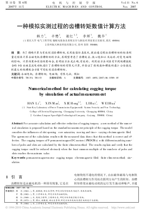
Num erical m ethod for calculating cogging torque by si m ulation of actual m easurem ent
A bstract : Fo r accurate calcu lation and effective reduct io n o f cogg ing torques , a new m ethod o f the nu m er ical si m ulat io n is proposed based on the standard m easure m ent prin ciple of the cogg ing torque . The m odel consid ers the influences of slot opening , core saturat io n , m ov ing and t i m e- varying e le ctrom agnetic filed . T he agree m ent of th e calcu lation results w ith the m easured data show s th at this m ethod is co rrect and ef fective. The cogging torques of 9 perm anent m agnet DC mo tors ( PMDCM s) w ith different m atch in g nu m bers o f po les and slots are calcu lated by the fin ite elem ent m ethod . The resu lts exp lain and verify th at the cogg ing torque cou ld be reduced obviously when the least comm on mu ltiple of the nu m bers of po les and slots reaches the m ax i m um va lu e . K ey w ord s : per m anent m agnet m oto r ; cogg ing torque ; e lectrom agnet ic filed ; fin ite e le m ent m ethod; si m ulat io n
齿轮齿条推力和扭矩计算
齿轮齿条推力和扭矩计算
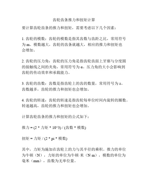
要计算齿轮齿条的推力和扭矩,需要考虑以下几个因素:
1. 齿轮的模数:齿轮的模数是指其齿数与齿距之比,常用符号为m。
模数越大,齿轮的齿条就越大,相应的推力和扭矩也
会增加。
2. 齿轮的压力角:齿轮的压力角是指齿轮齿面上牙廓与分度圆的接触线之间的夹角,常用符号为α。
压力角的大小会影响到
齿轮的传动效率和承载能力。
3. 齿轮的齿数:齿数是指齿轮上的齿的数量,常用符号为z。
齿数越多,齿轮的推力和扭矩也会增加。
4. 齿轮的转速:齿轮的转速是指齿轮每单位时间内旋转的圈数。
转速越高,齿轮的推力和扭矩也会增加。
计算齿轮齿条的推力和扭矩的公式如下:
推力 = (2 * 力矩 * 10^3) / (齿数 * 模数)
扭矩 = 力矩 / (2 * pi * 模数)
其中,力矩为施加在齿轮上的力与其半径的乘积。
推力的单位为牛顿(N),力矩的单位为牛顿·米(N·m),模数的单位为毫米(mm),齿数为无单位量。
需要注意的是,以上的公式仅适用于理想情况下的齿轮齿条,考虑到实际工程中的摩擦、传动损失等因素时,计算会更加复杂。
- 1、下载文档前请自行甄别文档内容的完整性,平台不提供额外的编辑、内容补充、找答案等附加服务。
- 2、"仅部分预览"的文档,不可在线预览部分如存在完整性等问题,可反馈申请退款(可完整预览的文档不适用该条件!)。
- 3、如文档侵犯您的权益,请联系客服反馈,我们会尽快为您处理(人工客服工作时间:9:00-18:30)。
Development of Analytical Equations to Calculate the Cogging Torquein Transverse Flux MachinesM. V. Ferreira da Luz (1), P. Dular (2), N. Sadowski (1), R. Carlson (1) and J. P. A. Bastos (1)(1) GRUCAD, Dept. of Electrical Engineering, Federal University of Santa Catarina, Brazil.(2) Dept. of Electrical Engineering and Computer Science, F.N.R.S., ULG, Belgium.Po. Box 476, 88040-900, Florianópolis, Santa Catarina, Brazil.E-mail of Corresponding Author: mauricio@grucad.ufsc.brAbstract - Cogging torque is produced in a permanent magnetmachine by magnetic attraction between the rotor permanentmagnets and the stator teeth. It is an undesirable effect thatcontributes to torque ripple, vibration and noise of the machine. In this paper, the resultant cogging torque values are computed using a three-dimensional (3D) finite element analysis. For this, the rotor movement is modeled by means of the moving bandtechnique in which a dynamic allocation of periodic or anti-periodic boundary conditions is performed. The 3D finite element method is the most accurate tool to carry out cogging torque. However, it does not easily allow a parametric study. For this reason, an analytical model was developed in order to predict the cogging torque. The tools are intended to be used for the study of transverse flux machines.I.I NTRODUCTIONAlthough permanent magnet (PM) machines are high performance devices, there are torque variations that affect their output performance. These variations during one revolution arise from factors as: commutation of the phase currents; ripple in the current waveform caused by chopping; variations in the reluctance of the magnetic circuit due to slotting as the rotor rotates. This last effect is called cogging [1]. Cogging torque arises from the interaction between permanent magnets and slotted iron structure and occurs in almost all types of PM motors. It manifests itself by the tendency of a rotor to align in a number of stable positions even when the machine is unexcited, and results in a pulsating torque, which does not contribute to the net effective torque. Therefore, one major task in developing PM machines is to minimize the cogging torque. Several methods are known. Some researchers minimize the cogging torque by skewing, an asymmetric distribution of the magnets or pole shifting [2]. Others works consider the relative air-gap permeance by modeling the shape of slots, the tooth width, or using teeth pairing, extra slots or notches in the teeth [3]. Others works control the function of the magnetization manipulating the shape of the magnets, the magnetization of the magnets themselves, the pole arc to pole pitch ratio, and the shape of the iron core [4].To verify the effects of machine geometry on the cogging torque is important to determinate its waveform. The electromagnetic torque can be calculated analytically or numerically in a variety of ways, such as Maxwell Stress and co-energy methods. However, they require very accurate global and local field solutions, particularly for the determination of cogging torque. In other words, a high level of mesh discretisation is required in a finite element method (FEM) calculation, whilst a reliable physical model is essential to an analytical prediction. A lot of work has been done on prediction of cogging torque in PM motors. They are divided into three groups. The first group uses analytical approaches [4, 5]. The second group uses the bi-dimensional (2D) and three-dimensional (3D) FEM simulation [6] and the third one uses a combined numerical and analytical method [7].In the last years we have developed a set of numerical tools for efficiently studying PM machines with FEM. A 3D magnetodynamic formulation, using the magnetic vector potential as the main unknown, discretized with edge finite elements, has been developed with adapted techniques for considering stranded conductors, periodicity and anti-peridodicity boundary conditions, moving band connection conditions and moving parts. The rotor displacement is modeled by means of a layer of finite elements placed in the air gap [8]. This method, named Moving Band Method, uses an automatic relocation of periodicity or anti-periodicity boundary conditions allowing the simulation of any displacement between stationary and moving parts of an electrical machine. The 3D FEM is the most accurate tool to carrying out cogging torque. However, it does not easily allow a parametric study. Moreover, the 3D simulation demands a high computation time. Hence, the purpose of this paper is to develop an analytical model and to compare it with 3D FEM for a transverse flux machine. This comparison allows finding an analytical model fast and precise to study the cogging torque behavior in order to satisfy some industrial design constraints for machines.The contribution of this paper could be divided in two aspects: the first one is the cogging torque calculation using the Moving Band Method for a 3D problem considering two moving bands in the same motor. The second aspect is the development of the analytical model to the transverse flux permanent magnet (TFPM) machine.TFPM machines have been found to be highly viable candidates in electric and hybrid propulsion applications [6]. Of particular interest are the double-sided topologies where high energy permanent magnets are mounted in the rotor rims in a flux concentration arrangement, yielding high air gap flux densities. The topology of such a machine requires 3D finiteelement analyses to accurately predict the machine parameters [6]. II. M AGNETODYNAMIC F ORMULATIONA bounded domain Ω of the two or three-dimensionalEuclidean space is considered. Its boundary is denoted Γ. Theequations characterising the magnetodynamic problem in Ω are[9]:j h = curl , b e t curl ∂−=, 0 div =b , (1a-b-c) r b h b +μ=, e j σ=, (2a-b)where h is the magnetic field, b is the magnetic flux density, b r is the permanent magnet remanent flux density, e is the electric field, j is the electric current density, including source currents j s in Ωs and eddy currents in Ωc (both Ωs and Ωc are included in Ω), μ is the magnetic permeability and σ is the electric conductivity.The boundary conditions are defined on complementary parts Γh and Γe , which can be non-connected, of Γ,0h =×Γh n , 0 . e =Γb n , 0e=×Γe n , (3a-b-c) where n is the unit normal vector exterior to Ω. Furthermore, global conditions on voltages or currents in inductors can be considered [8]. The a -formulation, with a magnetic vector potential a and an electric scalar potential v, is obtained from the weak form of the Ampère equation (1a) and (2a-b) [9], i.e.,0)' ,()' ,grad v ( )' , ( ',)' curl , ()' curl , url c (s h s c c t s r =−σ+∂σ+>×<+ν−νΩΩΩΓΩΩa j a a a a h n a b a a),(F 'a Ω∈∀awhere s h n × is a constraint on the magnetic field associated with boundary Γh of the domain Ω and μ=ν/1 is themagnetic reluctivity.F a (Ω) denotes the function space defined on Ω which contains the basis and test functions for both vector potentials a and a'. (. , .)Ω and <. , .>Γ denote a volume integral in Ω and a surface integral on Γ of products of scalar or vector fields.Using edge finite elements for a , a gauge condition associated with a tree of edges is generally applied.III. P ERIODICITY C ONDITIONS AND M OVING B AND M ETHOD Another important point is the simulation of the rotor movement. The applied technique permits the use of only one mesh for the calculation.Generally, to model electrical machines not presenting fractional windings, the calculation domain can be reduced to one or two poles using anti-periodic or periodic boundary conditions [9]. The discretisation of these boundaries is performed in a similar way, linking all their geometricalentities (nodes, edges and facets) by pairs. These boundaries are denoted ΓA and ΓB , respectively the reference boundary(which contains all the degrees of freedom) and its associatedboundary [8].For the a -formulation, periodicity conditions are split up into a strong relation on the normal component of b and a weakrelation on the tangential component of the magnetic field h .When edge finite elements are used for a , the strongperiodicity (anti-periodicity, with the other sign) relation for apair of equally oriented edges on ΓA and ΓB is a B = ± a A , (5) where a A and a B are the circulations of a along the considered edges on ΓA and ΓB . In 3D, periodicity conditions have to be consistent with gauge conditions (when used) associated with trees of edges [8].The periodicity boundary conditions can be directly applied to the moving band [8] connection (Fig. 1). The connection between the moving and the stationary regions (both being separately meshed), through the moving band, is similar to a periodicity connection (direct identification of the degrees offreedom; Fig. 1, boundaries b-b'). When (anti-) periodicity conditions are considered on both sides of the band (Fig. 1,boundaries a-a'), a complementary part of this band has to be connected through the same conditions to the moving region (Fig. 1, boundaries c-c') [8].Such connection conditions have to be updated for each position during the movement. When the calculation domain angle is exceeded, the moving part must be relocated in front of the stationary part, while inverting the connection conditions (i.e., inverting the rotor field sources) if anti-periodicity conditions are used.The movement is considered using the Lagrangian approach, i.e. with a moving coordinate system [10]. This approach is easily and implicitly considered with the a -formulation because no deformation is done in the domains involving the time derivative, i.e., in the conducting regions.IV. N UMERICAL P REDICTION OF C OGGING T ORQUE The cogging torque is computed at each angular position by means of 3D FEM analysis, integrating the Maxwell stress tensor on a surface containing the rotor, with null stator currents.To the aim of reducing the numerical errors, the cogging torque should be computed as the mean value of the Maxwellstress tensor on the whole airgap volume V g [9], i.e.∫∫∫∧=gV cogging dv )d (T F r , (6)where F is the Maxwell stress and the r is the dummy radius.V. A NALYTICAL P REDICTION OF C OGGING T ORQUE The cogging torque experienced by all estator teeth has the same shape, but are offset from each other in phase by the angular slot pitch [11]. The cogging torque experienced by the k th stator tooth can be written as the Fourier series()∑∞=ϕ+−+=θ1n n s n o ck )θn(θ2 cos T 2 T )(T , (7)where θ is the mechanical angular position of the rotor and ϕn is the phase angle of the k th harmonic component. T n are the Fourier series coefficients and they are determined by the magnetic field distribution around each tooth, the air gap length, and the size of the slot opening between teeth [11]. The method is based on the derivation of the flux density distributions in airgaps as a function of the machine design parameters. θs is the angular slot pitch calculated by sms N N π=θ, (8) where N m is the number of stator slots and N s is the number of magnet poles.Since the cogging torque of each tooth adds to create the net cogging torque of the motor, the motor cogging torque can be written as ∑−==θ1N 0k ck 2n cogging s )(θT S )(T , (9)where S 2n is the skew factor, which is given by ⎟⎟⎠⎞⎜⎜⎝⎛απαπ=s sk m sk m sn 2N N n sin N n N S , (10) where αsk is the slot pitches.In the analytical approach the assumptions used supposed that the end effects and the iron saturation are negligible.VI. R ESULTSThe analyzed TFPM machine as shown in Fig. 2 has 90 poles, a rated power of 10 kW, a rated voltage 220 V, and a rated speed of 200 rpm. This motor was manufactured by WEG Industries - Brazil. Fig. 3 shows a CAD model of the TFPM machine. Fig. 4 and Fig. 5 show the assembly details of the inner and outer stator for one phase of the TFPM machine. In this doubled-sided construction, the rotor is arranged between an inner and an outer stator.Figure 2. The TFPM machine manufactured by WEG Industries - Brazil.Figure 3. A CAD model of the TFPM machine.Figure 4. Assembly details of the inner and outer stator - one phase of theTFPM machine.Fig. 6 shows the ring-shaped windings of the TFPM machine.The Nd-Fe-B permanent magnets in the rotor are magnetized with an alternating polarity in circumferential direction. Therefore, the flux concentrating elements in the rotor increase the magnetic flux density in the airgaps beyond the remanent flux density of the Nd-Fe-B magnets. Fig. 7 shows the magnetic flux distribution due to the Nd-Fe-B magnets to the one-phase of TFPM machine.Figure 5. Assembly details of the inner stator - one phase of the TFPMmachine.Figure 6. Ring-shaped windings of the TFPM machine.Figure 7. Magnetic flux distribution to the one phase of the TFPM machine. The typical feature of TFPM machine is the magnetic flux path which has sections where the flux is transverse to the rotation plane and the ring-shaped winding in the stator in which the direction of the current corresponds to the movement direction of the rotor. This design leads to a structure in which the design of the magnetic circuit becomes almost independent from the design of the electrical circuit. Hence, there is the possibility to achieve higher torque values by increasing the number of pole pairs without affecting the electrical circuit parameters [12]. Also the absence of end-turns in stator winding which results in reduced copper losses is one of the major advantages of this machine structure.Considering the electromagnetic symmetries and using periodic boundary conditions, the smaller domain of study consists of an 8-degree sector of the whole structure. The 3D mesh without the air elements is shown in Fig. 8. In this figure we can see the stator, the coils, the rotor with the permanent magnets and the two moving bands (one inner and another external to the rotor). Each air gap was divided in three equal layers, being the moving band located in the central layer. Hexahedra in the moving band and prisms elsewhere have been used. The mesh of the structure has 40 divisions along the moving band.Figure 8. The studied domain and 3D mesh for TFPM machine. Results are presented for a speed of 200 rpm and when the machine operates at no-load condition, i.e. only the permanent magnet excitation is considered. Fig. 9 shows the cogging torque produced by both outer and inner parts of one phase.Figure 9. The cogging torque (normalized) produced by both outer and inner parts of one phase versus angle for TFPM machine.VII.C ONCLUSIONSIn this paper, the cogging torque was calculated with a 3D magnetodynamic formulation and with adapted techniques for considering stranded conductors, periodicity and anti-peridodicity boundary conditions, moving band connection conditions and moving parts. The Moving Band Method was implemented for 3D problems considering one or more moving bands in the same motor.The 3D FEM is the most accurate tool to carrying out cogging torque. However, it does not easily allow a parametric study. For this reason, an analytical model was developed in order to predict the cogging torque of TFPM machine. The comparison of the results between the analytical model and the 3D FEM simulation was satisfactory.Consequently, the developed analytical model allows fast and precise study of the influence of rotor permanent magnet distribution as well as the opening of stator auxiliary poles on the cogging torque behaviour in order to satisfy some industrial design constraints for machines. The skewing of the stator slots or, alternatively, of the permanent magnets also is taken into account with the analytical model.A CKNOWLEDGMENTThe authors thank the cooperation of the WEG Industries - Brazil. This work was supported by National Council for Scientific and Technological Development (CNPq) of Brazil.R EFERENCES[1] J. R. Hendershot Jr. and T. J. E. Miller, Design of Brushless Permanent-Magnet Motors, Magna Physics Publishing and Clarendon Press - Oxford, 1994.[2] N. Bianchi and S. Bolognani, “Design techniques for reducing thecogging torque in surface-mounted PM motors”, IEEE Transactions on Industry Applications, Vol. 38, No. 5, pp. 1259-1265, 2002.[3] R. Carlson, A. A. Tavares, J. P. A. Bastos and M. Lajoie-Mazenc.“Torque ripple attenuation in permanent magnet synchronous motors”.In: IEEE-IAS Annual Meeting, San Diego. Proceedings of IEEE-IAS, p.57-62, 1989.[4] S. M. Hwang, J. B. Eom, Y. H. Jung, D. W. Lee and B. S. Kang.“Various design techniques to reduce cogging torque by controlling energy variation in permanent magnet motors”. I EEE Transactions on Magnetics, Vol. 37, No. 4, pp. 2806-2809, 2001.[5] J. F. Gieras, “Analytical approach to cogging torque calculation of PMbrushless motors”. IEEE Transactions on Industry Applications, Vol. 40, No. 5, pp. 1310-1316, 2004.[6] E. Schmidt, “3-D Finite element analysis of the cogging torque of atransverse flux machine”. IEEE Transactions on Magnetics, Vol. 41. No.5, pp. 1836-1839, 2005.[7] C. Schlensok, M. H. Gracia and K. Hameyer, “Combined numerical andanalytical method for geometry optimization of a PM motor”. IEEE Transactions on Magnetics, Vol. 42, No. 4, pp. 1211-1214, 2006.[8] M. V. Ferreira da Luz, P. Dular, N. Sadowski, C. Geuzaine, J. P. A.Bastos, “Analysis of a permanent magnet generator with dual formulations using periodicity conditions and moving band”, IEEE Transactions on Magnetics, Vol. 38, No. 2, pp. 961-964, 2002.[9] J. P. A. Bastos and N. Sadowski, Electromagnetic Modeling by FiniteElements. Marcel Dekker, Inc, New York, USA, 2003.[10] K. Muramatsu, T. Nakata, N. Takahashi, and K. Fujiwara, “Comparisonof coordinate systems for eddy current analysis in moving conductors”, IEEE Transactions on Magnetics, Vol. 28, No. 2, pp. 1186-1189, 1992. [11] D. C. Halselman, Brushless Permanent Magnet Motor Design. SecondEdition, Published by The Writers’Collective, 2003.[12] M. Bork, G. Henneberger, “New transverse flux concept for an electricvehicle drive system”, ICEM 96 Proceedings, International Conference on Electrical Machines, Vol. 2, pp. 308-313, 1996.。