section2(博弈论讲义(Harvard University))汇总
博弈论2-2. sequential bargaining

2
大连理工
张醒洲
2014/3/5
动态博弈
博弈的扩展式表示 反向归纳法
3
大连理工
张醒洲
2014/3/5
序惯谈判
• 一个三阶段谈判模型 • 鲁宾斯坦 (1982)模型
2014/3/5
大连理工
张醒洲
4
一个三阶段谈判模型
参与人1和2就一美元的分配进行谈判。他们轮 流提出方案:首先参与人1提出一个分配方案,参 与人2可以接受或拒绝;如果参与人2拒绝,就由参 与人2提出分配建议,参与人1选择接受或拒绝;如 此进行下去。 一个方案一旦被拒绝,它就不再有任何约束力, 并与博弈后续进程不再相关。每一个方案都代表博 弈的一个阶段,参与人都没有足够的耐心:他们对 后面阶段得到的收益进行贴现,每一阶段的贴现因 子为δ,这里0 <δ< 1。
s2都可立即
拿到),或者拒绝这一条件(在这种情况下,博弈将继续 进行,进入第三阶段);
大连理工 张醒洲 7
一个三阶段谈判模型: 时间顺序
(3) 一旦进入第三阶段,参与人1得到美元的s
,参与人2得到1-s,这里 0 <
s
< 1。
大连理工
张醒洲
8
一个三阶段谈判模型
阶段 1
提议(s1, 1-s1)
阶段 2
• 如果第3阶段开始的博弈均衡是( s, 1-s)的话,前述三 阶段博弈开始时第1人的最优方案是(1-δ(1- δs), δ(1- δs)) • 对无限期讨价还价博弈,第一阶段开始时参与者1提出的 最优方案是s, 且有
S= (1-δ(1- δs), δ(1- δs)) 即 S= 1/(1+δ)
2014/3/5 大连理工 张醒洲 13
lecture_2(博弈论讲义GameTheory(MIT))
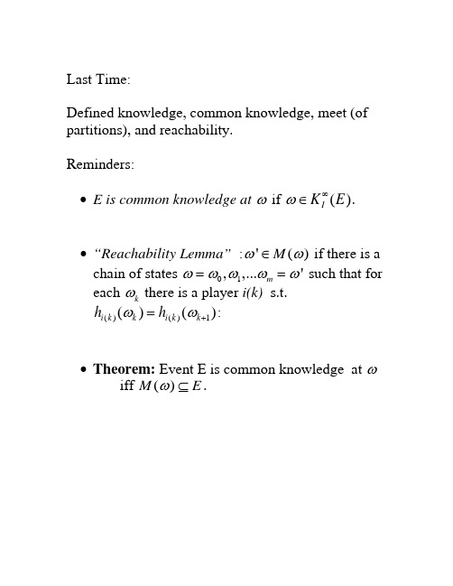
Last Time:Defined knowledge, common knowledge, meet (of partitions), and reachability.Reminders:• E is common knowledge at ω if ()I K E ω∞∈.• “Reachability Lemma” :'()M ωω∈ if there is a chain of states 01,,...m 'ωωωωω== such that for each k ω there is a player i(k) s.t. ()()1()(i k k i k k h h )ωω+=:• Theorem: Event E is common knowledge at ωiff ()M E ω⊆.How does set of NE change with information structure?Suppose there is a finite number of payoff matrices 1,...,L u u for finite strategy sets 1,...,I S SState space Ω, common prior p, partitions , and a map i H λso that payoff functions in state ω are ()(.)u λω; the strategy spaces are maps from into . i H i SWhen the state space is finite, this is a finite game, and we know that NE is u.h.c. and generically l.h.c. in p. In particular, it will be l.h.c. at strict NE.The “coordinated attack” game8,810,11,100,0A B A B-- 0,010,11,108,8A B A B--a ub uΩ= 0,1,2,….In state 0: payoff functions are given by matrix ; bu In all other states payoff functions are given by . a upartitions of Ω1H : (0), (1,2), (3,4),… (2n-1,2n)... 2H (0,1),(2,3). ..(2n,2n+1)…Prior p : p(0)=2/3, p(k)= for k>0 and 1(1)/3k e e --(0,1)ε∈.Interpretation: coordinated attack/email:Player 1 observes Nature’s choice of payoff matrix, sends a message to player 2.Sending messages isn’t a strategic decision, it’s hard-coded.Suppose state is n=2k >0. Then 1 knows the payoffs, knows 2 knows them. Moreover 2 knows that 1knows that 2 knows, and so on up to strings of length k: . 1(0n I n K n -Î>)But there is no state at which n>0 is c.k. (to see this, use reachability…).When it is c.k. that payoff are given by , (A,A) is a NE. But.. auClaim: the only NE is “play B at every information set.”.Proof: player 1 plays B in state 0 (payoff matrix ) since it strictly dominates A. b uLet , and note that .(0|(0,1))q p =1/2q >Now consider player 2 at information set (0,1).Since player 1 plays B in state 0, and the lowest payoff 2 can get to B in state 1 is 0, player 2’s expected payoff to B at (0,1) is at least 8. qPlaying A gives at most 108(1)q q −+−, and since , playing B is better. 1/2q >Now look at player 1 at 1(1,2)h =. Let q'=p(1|1,2), and note that '1(1)q /2εεεε=>+−.Since 2 plays B in state 1, player 1's payoff to B is at least 8q';1’s payoff to A is at most -10q'+8(1-q) so 1 plays B Now iterate..Conclude that the unique NE is always B- there is no NE in which at some state the outcome is (A,A).But (A,A ) is a strict NE of the payoff matrix . a u And at large n, there is mutual knowledge of the payoffs to high order- 1 knows that 2 knows that …. n/2 times. So “mutual knowledge to large n” has different NE than c.k.Also, consider "expanded games" with state space . 0,1,....,...n Ω=∞For each small positive ε let the distribution p ε be as above: 1(0)2/3,()(1)/3n p p n ee e e -==- for 0 and n <<∞()0p ε∞=.Define distribution by *p *(0)2/3p =,. *()1/3p ∞=As 0ε→, probability mass moves to higher n, andthere is a sense in which is the limit of the *p p εas 0ε→.But if we do say that *p p ε→ we have a failure of lower hemi continuity at a strict NE.So maybe we don’t want to say *p p ε→, and we don’t want to use mutual knowledge to large n as a notion of almost common knowledge.So the questions:• When should we say that one information structure is close to another?• What should we mean by "almost common knowledge"?This last question is related because we would like to say that an information structure where a set of events E is common knowledge is close to another information structure where these events are almost common knowledge.Monderer-Samet: Player i r-believes E at ω if (|())i p E h r ω≥.()r i B E is the set of all ω where player i r- believesE; this is also denoted 1.()ri B ENow do an iterative definition in the style of c.k.: 11()()rr I i i B E B E =Ç (everyone r-believes E) 1(){|(()|())}n r n ri i I B E p B E h r w w -=³ ()()n r n rI i i B E B =ÇEE is common r belief at ω if ()rI B E w ¥ÎAs with c.k., common r-belief can be characterized in terms of public events:• An event is a common r-truism if everyone r -believes it when it occurs.• An event is common r -belief at ω if it is implied by a common r-truism at ω.Now we have one version of "almost ck" : An event is almost ck if it is common r-belief for r near 1.MS show that if two player’s posteriors are common r-belief, they differ by at most 2(1-r): so Aumann's result is robust to almost ck, and holds in the limit.MS also that a strict NE of a game with knownpayoffs is still a NE when payoffs are "almost ck” - a form of lower hemi continuity.More formally:As before consider a family of games with fixed finite action spaces i A for each player i. a set of payoff matrices ,:l I u A R ->a state space W , that is now either finite or countably infinite, a prior p, a map such that :1,,,L l W®payoffs at ω are . ()(,)()w u a u a l w =Payoffs are common r-belief at ω if the event {|()}w l w l = is common r belief at ω.For each λ let λσ be a NE for common- knowledgepayoffs u .lDefine s * by *(())s l w w s =.This assigns each w a NE for the corresponding payoffs.In the email game, one such *s is . **(0)(,),()(,)s B B s n A A n ==0∀>If payoffs are c.k. at each ω, then s* is a NE of overall game G. (discuss)Theorem: Monder-Samet 1989Suppose that for each l , l s is a strict equilibrium for payoffs u λ.Then for any there is 0e >1r < and 1q < such that for all [,1]r r Î and [,1]q q Î,if there is probability q that payoffs are common r- belief, then there is a NE s of G with *(|()())1p s s ωωω=>ε−.Note that the conclusion of the theorem is false in the email game:there is no NE with an appreciable probability of playing A, even though (A,A) is a strict NE of the payoffs in every state but state 0.This is an indirect way of showing that the payoffs are never ACK in the email game.Now many payoff matrices don’t have strictequilibria, and this theorem doesn’t tell us anything about them.But can extend it to show that if for each state ω, *(s )ω is a Nash (but not necessarily strict Nash) equilibrium, then for any there is 0e >1r < and 1q < such that for all [,1]r r Î and [,1]q q Î, if payoffs are common r-belief with probability q, there is an “interim ε equilibria” of G where s * is played with probability 1ε−.Interim ε-equilibria:At each information set, the actions played are within epsilon of maxing expected payoff(((),())|())((',())|())i i i i i i i i E u s s h w E u s s h w w w w e-->=-Note that this implies the earlier result when *s specifies strict equilibria.Outline of proof:At states where some payoff function is common r-belief, specify that players follow s *. The key is that at these states, each player i r-believes that all other players r-believe the payoffs are common r-belief, so each expects the others to play according to s *.*ΩRegardless of play in the other states, playing this way is a best response, where k is a constant that depends on the set of possible payoff functions.4(1)k −rTo define play at states in */ΩΩconsider an artificial game where players are constrained to play s * in - and pick a NE of this game.*ΩThe overall strategy profile is an interim ε-equilibrium that plays like *s with probability q.To see the role of the infinite state space, consider the"truncated email game"player 2 does not respond after receiving n messages, so there are only 2n states.When 2n occurs: 2 knows it occurs.That is, . {}2(0,1),...(22,21,)(2)H n n =−−n n {}1(0),(1,2),...(21,2)H n =−.()2|(21,2)1p n n n ε−=−, so 2n is a "1-ε truism," and thus it is common 1-ε belief when it occurs.So there is an exact equilibrium where players playA in state 2n.More generally: on a finite state space, if the probability of an event is close to 1, then there is high probability that it is common r belief for r near 1.Not true on infinite state spaces…Lipman, “Finite order implications of the common prior assumption.”His point: there basically aren’t any!All of the "bite" of the CPA is in the tails.Set up: parameter Q that people "care about" States s S ∈,:f S →Θ specifies what the payoffs are at state s. Partitions of S, priors .i H i pPlayer i’s first order beliefs at s: the conditional distribution on Q given s.For B ⊆Θ,1()()i s B d =('|(')|())i i p s f s B h s ÎPlayer i’s second order beliefs: beliefs about Q and other players’ first order beliefs.()21()(){'|(('),('))}|()i i j i s B p s f s s B h d d =Îs and so on.The main point can be seen in his exampleTwo possible values of an unknown parameter r .1q q = o 2qStart with a model w/o common prior, relate it to a model with common prior.Starting model has only two states 12{,}S s s =. Each player has the trivial partition- ie no info beyond the prior.1122()()2/3p s p s ==.example: Player 1 owns an asset whose value is 1 at 1θ and 2 at 2θ; ()i i f s θ=.At each state, 1's expected value of the asset 4/3, 2's is 5/3, so it’s common knowledge that there are gains from trade.Lipman shows we can match the players’ beliefs, beliefs about beliefs, etc. to arbitrarily high order in a common prior model.Fix an integer N. construct the Nth model as followsState space'S ={1,...2}N S ´Common prior is that all states equally likely.The value of θ at (s,k) is determined by the s- component.Now we specify the partitions of each player in such a way that the beliefs, beliefs about beliefs, look like the simple model w/o common prior.1's partition: events112{(,1),(,2),(,1)}...s s s 112{(,21),(,2),(,)}s k s k s k -for k up to ; the “left-over” 12N -2s states go into 122{(,21),...(,2)}N N s s -+.At every event but the last one, 1 thinks the probability of is 2/3.1qThe partition for player 2 is similar but reversed: 221{(,21),(,2),(,)}s k s k s k - for k up to . 12N -And at all info sets but one, player 2 thinks the prob. of is 1/3.1qNow we look at beliefs at the state 1(,1)s .We matched the first-order beliefs (beliefs about θ) by construction)Now look at player 1's second-order beliefs.1 thinks there are 3 possible states 1(,1)s , 1(,2)s , 2(,1)s .At 1(,1)s , player 2 knows {1(,1)s ,2(,1)s ,(,}. 22)s At 1(,2)s , 2 knows . 122{(,2),(,3),(,4)}s s s At 2(,1)s , 2 knows {1(,2)s , 2(,1)s ,(,}. 22)sThe support of 1's second-order beliefs at 1(,1)s is the set of 2's beliefs at these info sets.And at each of them 2's beliefs are (1/3 1θ, 2/3 2θ). Same argument works up to N:The point is that the N-state models are "like" the original one in that beliefs at some states are the same as beliefs in the original model to high but finite order.(Beliefs at other states are very different- namely atθ or 2 is sure the states where 1 is sure that state is2θ.)it’s1Conclusion: if we assume that beliefs at a given state are generated by updating from a common prior, this doesn’t pin down their finite order behavior. So the main force of the CPA is on the entire infinite hierarchy of beliefs.Lipman goes on from this to make a point that is correct but potentially misleading: he says that "almost all" priors are close to a common. I think its misleading because here he uses the product topology on the set of hierarchies of beliefs- a.k.a topology of pointwise convergence.And two types that are close in this product topology can have very different behavior in a NE- so in a sense NE is not continuous in this topology.The email game is a counterexample. “Product Belief Convergence”:A sequence of types converges to if thesequence converges pointwise. That is, if for each k,, in t *i t ,,i i k n k *δδ→.Now consider the expanded version of the email game, where we added the state ∞.Let be the hierarchy of beliefs of player 1 when he has sent n messages, and let be the hierarchy atthe point ∞, where it is common knowledge that the payoff matrix is .in t ,*i t a uClaim: the sequence converges pointwise to . in t ,*i t Proof: At , i’s zero-order beliefs assignprobability 1 to , his first-order beliefs assignprobability 1 to ( and j knows it is ) and so onup to level n-1. Hence as n goes to infinity, thehierarchy of beliefs converges pointwise to common knowledge of .in t a u a u a u a uIn other words, if the number of levels of mutual knowledge go to infinity, then beliefs converge to common knowledge in the product topology. But we know that mutual knowledge to high order is not the same as almost common knowledge, and types that are close in the product topology can play very differently in Nash equilibrium.Put differently, the product topology on countably infinite sequences is insensitive to the tail of the sequence, but we know that the tail of the belief hierarchy can matter.Next : B-D JET 93 "Hierarchies of belief and Common Knowledge”.Here the hierarchies of belief are motivated by Harsanyi's idea of modelling incomplete information as imperfect information.Harsanyi introduced the idea of a player's "type" which summarizes the player's beliefs, beliefs about beliefs etc- that is, the infinite belief hierarchy we were working with in Lipman's paper.In Lipman we were taking the state space Ω as given.Harsanyi argued that given any element of the hierarchy of beliefs could be summarized by a single datum called the "type" of the player, so that there was no loss of generality in working with types instead of working explicitly with the hierarchies.I think that the first proof is due to Mertens and Zamir. B-D prove essentially the same result, but they do it in a much clearer and shorter paper.The paper is much more accessible than MZ but it is still a bit technical; also, it involves some hard but important concepts. (Add hindsight disclaimer…)Review of math definitions:A sequence of probability distributions converges weakly to p ifn p n fdp fdp ®òò for every bounded continuous function f. This defines the topology of weak convergence.In the case of distributions on a finite space, this is the same as the usual idea of convergence in norm.A metric space X is complete if every Cauchy sequence in X converges to a point of X.A space X is separable if it has a countable dense subset.A homeomorphism is a map f between two spaces that is 1-1, and onto ( an isomorphism ) and such that f and f-inverse are continuous.The Borel sigma algebra on a topological space S is the sigma-algebra generated by the open sets. (note that this depends on the topology.)Now for Brandenburger-DekelTwo individuals (extension to more is easy)Common underlying space of uncertainty S ( this is called in Lipman)ΘAssume S is a complete separable metric space. (“Polish”)For any metric space, let ()Z D be all probability measures on Borel field of Z, endowed with the topology of weak convergence. ( the “weak topology.”)000111()()()n n n X S X X X X X X --=D =´D =´DSo n X is the space of n-th order beliefs; a point in n X specifies (n-1)st order beliefs and beliefs about the opponent’s (n-1)st order beliefs.A type for player i is a== 0012(,,,...)()n i i i i n t X d d d =¥=δD0T .Now there is the possibility of further iteration: what about i's belief about j's type? Do we need to add more levels of i's beliefs about j, or is i's belief about j's type already pinned down by i's type ?Harsanyi’s insight is that we don't need to iterate further; this is what B-D prove formally.Coherency: a type is coherent if for every n>=2, 21marg n X n n d d --=.So the n and (n-1)st order beliefs agree on the lower orders. We impose this because it’s not clear how to interpret incoherent hierarchies..Let 1T be the set of all coherent typesProposition (Brandenburger-Dekel) : There is a homeomorphism between 1T and . 0()S T D ´.The basis of the proposition is the following Lemma: Suppose n Z are a collection of Polish spaces and let021201...1{(,,...):(...)1, and marg .n n n Z Z n n D Z Z n d d d d d --´´-=ÎD ´"³=Then there is a homeomorphism0:(nn )f D Z ¥=®D ´This is basically the same as Kolmogorov'sextension theorem- the theorem that says that there is a unique product measure on a countable product space that corresponds to specified marginaldistributions and the assumption that each component is independent.To apply the lemma, let 00Z X =, and 1()n n Z X -=D .Then 0...n n Z Z X ´´= and 00n Z S T ¥´=´.If S is complete separable metric than so is .()S DD is the set of coherent types; we have shown it is homeomorphic to the set of beliefs over state and opponent’s type.In words: coherency implies that i's type determines i's belief over j's type.But what about i's belief about j's belief about i's type? This needn’t be determined by i’s type if i thinks that j might not be coherent. So B-D impose “common knowledge of coherency.”Define T T ´ to be the subset of 11T T ´ where coherency is common knowledge.Proposition (Brandenburger-Dekel) : There is a homeomorphism between T and . ()S T D ´Loosely speaking, this says (a) the “universal type space is big enough” and (b) common knowledge of coherency implies that the information structure is common knowledge in an informal sense: each of i’s types can calculate j’s beliefs about i’s first-order beliefs, j’s beliefs about i’s beliefs about j’s beliefs, etc.Caveats:1) In the continuity part of the homeomorphism the argument uses the product topology on types. The drawbacks of the product topology make the homeomorphism part less important, but theisomorphism part of the theorem is independent of the topology on T.2) The space that is identified as“universal” depends on the sigma-algebra used on . Does this matter?(S T D ´)S T ×Loose ideas and conjectures…• There can’t be an isomorphism between a setX and the power set 2X , so something aboutmeasures as opposed to possibilities is being used.• The “right topology” on types looks more like the topology of uniform convergence than the product topology. (this claim isn’t meant to be obvious. the “right topology” hasn’t yet been found, and there may not be one. But Morris’ “Typical Types” suggests that something like this might be true.)•The topology of uniform convergence generates the same Borel sigma-algebra as the product topology, so maybe B-D worked with the right set of types after all.。
第2章博弈论

最小得益最大化策略(Maxmin Strategy)
博弈的策略不仅取决于自己的理性,
而且取决于对手的理性。
如某电力局在考虑要不要在江边建一
座火力发电站,港务局在考虑要不要在江
边扩建一个煤码头。
完全信息静态对策----纯策略
电力局建电厂是上策。港务局 应当可以期望电力局建电厂,因 此也选择扩建。 (建电厂,扩建)是纳什均衡。 但万一电力局不理性,选择 不建厂,港务局的损失太大了。 如你处在港务局的地位,一个 谨慎的做法是什么呢? 就是最小得益最大化策略。 电力局
混合策略博弈的几个原则
在“混合策略” 博弈中,每一个对局者的策略组合都不可能 是单一的策略或者纯策略,而必须把不同的策略混合一起使用。 任何一个对局者都必须遵循以下三个原则。 第一,不能让对方事先知道自己可能采取的策略。 第二,必须采取随机选择的原则。 第三,选择策略的概率一定要使对方无机可乘。即一方选择 的概率使对方无法通过选择某一策略而占有优势。也就是说,从 随机选择的角度来说,这意味着一方所选择策略的概率要使另一 方选择的所有策略的预期收益相等。 混合策略纳什均衡的现实意义在于,在不确定的经济环境中, 厂商的决策必须带有不可预测性。也就是说,厂商的决策必须出 其不意,攻其不备,才能使竞争对手措手不及,从而才能保证企 业在激烈的竞争中立于不败之地。但要使厂商的决策是不可预测 的,就要求厂商拥有其竞争对手不知道的未公开的信息,这些信 息的价值决定了决策不可预测性的程度。
纯策略的纳什均衡的求解方法之一:画线法
对于两个人的博弈,当每个纯策略集元素个数不是很多时, 可用穷举法即逐个挑出每个局中人每个策略下另一局中人的最优 策略,在其收益下加一横线,最后发现哪个格子内有两条横线, 即得纯策略N.E均衡
博弈论讲义入门 slides2

学生的成绩就是 其中, 是学生报出的数字。
VNM公理
• 公理A2(独立性):对任意p,q,r∈P,和 任意a∈(0,1],
VNM公理
• 公里A3(连续性):对任意p,q,r∈P,如 果 p > q > r,那么存在a,b∈(0,1) 使
定理—VNM表示
• P上的关系≥可用VNM效用函数u:Z→R 表示的充分必要条件是它满足公理A1-A3。 • u和v表示≥的充分必要条件是 其中a>0,b∈R
习题
• 考虑一正实数上可用VNM效用函数 u(x)=x2表示的关系≥。 这种关系可用VNM函数 表 示吗? 用 表示又如何呢?
对风险的态度
• 公平赌博:
• 参与者是风险中性的 iff 他对所有公平赌博无 所谓。 • 他是(严格)厌恶风险的 iff 他从不想参与公平赌 博。 • 他是(严格)追逐风险的 iff 他总是想参与公平赌 博。
基本概念:偏好 • 关系≥ (X上)是X×X上的任一子集 • 例如, • T≥C≡(T,C)∈≥ • ≥是完全的iff 要么X≥Y,要么Y≥X • ≥是传递的iff [X≥Y和Y≥Z]
偏好关系
• 定义:一种关系是偏好关系的充分必要 条件是,它是完全和传递的。
实例
• 在本班学生中定义下列关系 • xTy表示x至少和y一样高; • xMy表示x在课程14.04的期末成绩至少和 y一样高; • xHy表示x和y 上的同一所中学; • xYy表示x比y年龄小; • xSy表示x与y 同龄;
实例
可由函数u**表示,其中
练习
• 设想一群学生围绕一张圆桌坐下。定义 一种关系R,写成xRy,表示x坐在y的右 边。你能用一效用函数表示R吗? • 考虑一在正实数上以u表示的关系≥,其 中u(x)=x2。 • 这种关系可表示为 吗? • u**(x)=1/x 又 如何呢?
博弈论第2章

• 托玛斯 谢林(Thomas C. Schelling )84岁,美国公民。他1951年 托玛斯-谢林( 谢林 岁 美国公民。 年 获得哈佛大学经济学博士学位。 获得哈佛大学经济学博士学位。后曾在美国哈佛大学的肯尼迪学 院教学长达20 20年 担任政治经济学教授, 院教学长达20年,担任政治经济学教授,并获得退休名誉教授 的称号。之后他还在美国马里兰大学公共政策学院和经济系担任 的称号。 教授,并获得退休名誉教授称号。 教授,并获得退休名誉教授称号。他教授的课程除包括经济学理 论外,还涉及外交、国家安全、核战略以及军控等多方面。 论外,还涉及外交、国家安全、核战略以及军控等多方面。
贡献:《冲突战略》、《武器与影响》等,其中前者是相关领域中最具 开创性的理论著作之一。他的理论和思想不仅运用在经济学分析中,在外 交、军事领域也深有影响。
Robert J. Aumann
Thomas C. Schelling
罗伯特·奥曼的博弈论
• • • • • 弈论:交互式条件下“最优理性决策” 完全竞争经济:参与者连续统模型 重复博弈论:理论系统性的发展 合作与非合作博弈论:非转移效用与理性的假设 其他贡献 “奥曼可衡量选择定理”、值集函数积分结 果等 评论:
博弈论的形成
博弈论的真正起点 博弈论的真正起点—— 真正起点—— 诺伊曼、 1944年 冯 诺伊曼、摩根斯坦 1944年《博弈论和经济行 Behavior) 为》 (Theory of Games and Economic Behavior) 在这本著作中引进了扩展形(Extensive Form)表 在这本著作中引进了扩展形( 扩展形 ) 示和正规形(Normal Form)或称策略形(Strategy 示和正规形( )或称策略形( 正规形 Form)、矩阵形(Matrix Form)表示,定义了极小化 )、矩阵形 )、矩阵形( )表示,定义了极小化 ),提出了稳定集( 极大解( ),提出了稳定集 极大解(Minmax Solution),提出了稳定集(Stable Sets)解概念等,正式提出了创造一种博弈论的一般理 )解概念等, 论的主意
博弈论讲义共125页PPT

3、信息(Information):信息是参与人有关博 弈的知识,特别是有关自然的选择、其他参与 人的特征和行动的知识。
完全信息:每一个参与人对所有其他参与人 (包括自然)的特征、策略空间及支付函数有 准确的知识。否则,就是不完全信息。
共同知识:指的是所有参与人知道,而且所 有参与人知道所有参与人知道……的知识。 共同知识是一个非常强的假定。
案例
房地产开发项目-假设有A、B两家开发商 市场需求:可能大,也可能小 投入:1亿
❖假定市场上有两栋楼出售: ✓需求大时,每栋售价1.4亿, ✓需求小时,售价7千万; ❖如果市场上只有一栋楼 ✓需求大时,可卖1.8亿 ✓需求小时,可卖1.1亿
一 、博弈的基本概念及策略表述
博弈论的基本概念包括:
如果另一个犯罪嫌疑人也作了坦白,则两人 各被判刑8年;如果另一个犯罪嫌人没有坦 白而是抵赖,则以妨碍公务罪(因已有证据 表明其有罪)再加刑2年,而坦白者有功被 减刑8年,立即释放。如果两人都抵赖,则 警方因证据不足不能判两人的偷窃罪,但可 以私入民宅的罪名将两人各判入狱1年。
如何描述这个博弈? 他们将如何选择?
用博弈规则决定均衡。
1、参与人(Players):在博弈中独立决策、 独立承担博弈结果的个人或组织。也称局中 人。参与人的目的是通过选择行动或策略( 策略)以最大化自己的支付(效用)水平。 特殊的虚拟参与人-自然,其实质是决定 外生的环境参数的概率分布的一种机制。 i=1, ……, n代表参与人;N代表自然。
一 、博弈的基本概念及策略表述
博弈的策略式表述:
战略式表述给出: 1、博弈的参与人集合i:, (1,2,,n); 2、每个参与人的战略间空:Si,i 1,2,,n; 3、每个参与人的支付数函:ui (s1,, si,, sn),i 1,2,,n)
博弈论导论 2
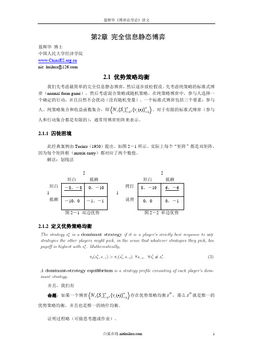
图 2-5 军备竞赛
思考:现实生活中还有哪些情况属于囚徒困境? 练习:将团队生产问题模型化成囚徒困境;如何理解囚徒困境与“看不见的手”之间 的矛盾?
2.1.5 走出囚徒困境
从社会福利的角度讲,囚徒困境不是帕累托最优的,但这与理性人的假设并不矛盾。
① ②
这实际上是 Betrand 价格竞争模型。 这是 Hardin(1968)发表在 Science 上但是被经济学引用最多的例子。但是,最近有学者提出了“反公地 悲剧”理论。董志强(2007)启发我使用这个简单的收益矩阵而非复杂的数学模型。 白鲨在线 2
2.3.2 性别战
如图 2-12。两个博弈相同的地方在于:(1)存在多重均衡,而且双方各自偏向一个 均衡;(2)任何一个均衡结果都是帕累托最优的。信念扮演了重要的作用。在这个博弈中, 假设男方是一个有名的拳击手,而女方也知道这点,那么(拳击,拳击)应该是一个均衡结 果,而(芭蕾,拳击)不应该出现。
白鲨在线 5
2.3.4 协调博弈
如图 2-14,史密斯公司和琼斯公司独立地决定选择何种智能手机操作系统。若两家公 司选择同样的操作系统,销售会更好。 特征:存在多重均衡,但是一些均衡帕累托优于另一些均衡,这与性别战和斗鸡博弈 都不同。 提示:一定要注意不同博弈模型的结构性特征,而不是过于关注具体数字。 思考:现实生活中有哪些博弈是性别战、斗鸡博弈和协调博弈?
图 2-1 双边优势
图 2-2 单边优势
2.1.2 定义优势策略均衡
并且,我们有 命题:如果一个博弈 N ,{Si }i 1 ,{vi ()}i 1 存在优势策略均衡 s ,那么 s 就是惟一的 优势策略均衡,并且也是惟一的纳什均衡。 证明过程略(可做思考题或作业)。
白鲨在线 1
复旦大学-谢识予-经济博弈论2

两寡头间的囚徒困境博弈
厂 不突破 商 1 突破
厂商2
不突破
突破
4.5,4.5
3.75,5
5,3.75
4,4
以自身最大利益为目标:各生产 2单位产量,各自得益为4
以两厂商总体利益最大:各生产 1.5单位产量,各自得益为4.5
2.3.2 反应函数
古诺模型的反应函数
max q1
u1
max(6q1
q1q2
2.4 混合策略和混合策略纳什均衡
2.4.1 严格竞争博弈和混合策略的引进 2.4.2 多重均衡博弈和混合策略 2.4.3 混合策略和严格下策反复消去法 2.4.4 混合策略反应函数
2.4.1 严格竞争博弈和混合策略的引进
一、猜硬币博弈
盖 正面 硬 币 反面 方
猜硬币方
正面
反面
-1, 1
1, -1
-1, -1
之
境
争
猜
-1, 1
硬
币
1, -1
1, -1 -1, 1
2, 1 0, 0
0, 0 1, 3
2.2 纳什均衡
2.2.1 纳什均衡的定义 2.2.2 纳什均衡的一致预测性质 2.2.3 纳什均衡与严格下策反复消去法
2.2.1 纳什均衡的定义
策略空间:S1 , S n
博弈方 i的第 j 个策略:si j Si 博弈方 i的得益:u i
博弈:G {S1,Sn;u1,un}
纳什均衡:在博弈G {S1,Sn;u1,un}中,如果由各个博弈方i
的各一个策略组成的某个策略组合(si*,sn* ) 中,任一博弈方 的策略,都是对其余博弈方策略的组合 (si*,si*1, si*1,...sn* ) 的最佳对策,也即ui (si*,si*1, si*, si*1,...sn*) ui (si*,si*1, sij , si*1,...sn*)
- 1、下载文档前请自行甄别文档内容的完整性,平台不提供额外的编辑、内容补充、找答案等附加服务。
- 2、"仅部分预览"的文档,不可在线预览部分如存在完整性等问题,可反馈申请退款(可完整预览的文档不适用该条件!)。
- 3、如文档侵犯您的权益,请联系客服反馈,我们会尽快为您处理(人工客服工作时间:9:00-18:30)。
• Pareto efficiency
Partnership Game: Setting
• • • • 2 Partners in business Complete information about the situation Simultaneous moves (no verifiable contract) Two players: i, j
– Those that survive iterated dominance – Motivated by common knowledge assumptions
• Congruity
– Weakly congruous strategies
• Each strategy is a best response to others’ strategy
– Partnership game – Cournot game
• Mixed strategy equilibria
– Conceptualization – How to solve – Application: Iran and IAEA
Key Terms and Definitions
• Set of rationalizable strategies
GOV 2005: Game Theory
Section 2: Externalities
Alexis Diamond adiamond@
Agenda
• Key terms and definitions • Complementarity and cross-partial derivatives)
Externalities: The Dirty Little Secret
When One Person’s Actions Affect Others’ Welfare
• • • • • •
Classic Examples Pollution Lightening rods Security Grades and curving LaTeX and presentations Cooperation and competition
– Each expends effort: i, j – Payoffs are: πi = 2(i + j + cij) - i2 πj = 2(i + j + cij) - j2
• Interpret these equations
Partnership Game: Analysis
• Payoffs are:
Contextual Strategic Issues • Complementarity
– Agents share the benefits of each other’s actions
• Substitutability
– Agents share the costs of each other’s actions
• πi = 2(i + j + cij) - i2 • πj = 2(i + j + cij) - j2
• Best response functions:
– d (πi)/di = 2+2cj - 2i – set equal to zero: 2i = 2 + 2cj
• i*=1+cj … This is our BR function for agent i
– symmetry requires that j*=1+ci
• If each is responding to the BR of the other
• j*=1+c(1+cj*), j*=1/(1-c) = i* also by symmetry • πi,j= 2[1/(1-c) + 1/(1-c) + c(1/(1-c))2] - (1/(1-c))2 • πi,j= (3-2c)/(1-c)2
Nash Eqm (TR & DC)
strategy profiles
Pareto Optima
Set of Rationalizable Strategies: {T,D} x {C,R} Set of Weakly Congruent Strategies: {T,D} x {C,R} Set of Best Response Complete: {T,D} x {C, R} or {T,D} x {L,C,R} Set of Congruent Strategies: {T,D} x {C, R}
– Best response complete
• Set includes i’s best response to all hers’ strategies
Quick Congruity Quiz
Player 2 Left Player 1 Top Middle Down 3,4 2,5 8,2 Center 2,3 -1,8 4,4 Right 9,15 4,0 5,0
Partnership Game: Pareto-Efficiency
In Strategic Setting, Equilibrium was i*,j*=1/(1-c), πi,j= (3-2c)/(1-c)2
• Now we leave the strategic setting (S.S.) and maximize total profits (pareto efficiency)
πF = 4(i + j + cij) - i2- j2
• d (πF)/di = 4 +4cj - 2i • d (πF)/dj = 4 +4ci - 2j
Set equal to zero: 2i = 4 + 4cj
• • • • i* = 2 + 2cj, j* = 2 + 2ci, i* = 2 + 2c(2 + 2ci*) i* = 2/(1-2c) = j*, πF = 8/(1-2c), Profit per partner, πi.j= 4/(1-2c) > (3-2c)/(1-c)2 in S.S. Note that output is also lower in the strategic setting