基于COMSOLMultiphysic电涡流传感器的仿真和设计
电涡流位移传感器设计
电涡流位移传感器设计技术要求:1、量程:0~20mm2、精度:1mm3、激励频率:1M Hz4、输入电压:24V5、介质温度: -50℃~250℃6、表面的粗糟度: 0.4μm~0.8μm7、线性误差:<±2%8、工作温度:探头(-20~120)℃,延长电缆(-20~120)℃,前置器(-30~50)℃9、频率响应:0~5KHz一、总体设计方案电涡流传感器能静态和动态地非接触、高线性度、高分辨力地测量被测金属导体距探头表面的距离。
它是一种非接触的线性化计量工具。
电涡流传感器能准确测量被测体(必须是金属导体)与探头端面之间静态和动态的相对位移变化。
电涡流传感器以其长期工作可靠性好、测量范围宽、灵敏度高、分辨率高、响应速度快、抗干扰力强、不受油污等介质的影响、结构简单等优点。
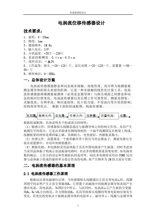
根据下面的组成框图,构成传感器。
根据组成框图,具体说明各个组成部分的材料:(1)敏感元件:传感器探头线圈是通过与被测导体之间的相互作用,从而产生被测信号的部分,它是由多股漆包铜线绕制的一个扁平线圈固定在框架上构成,线圈框架的材料是聚四氟乙烯,其顺耗小,电性能好,热膨胀系数小。
(2)传感元件: 前置器是一个能屏蔽外界干扰信号的金属盒子,测量电路完全装在前置器中,并用环氧树脂灌封。
(3)测量电路:本电路拟采用晶体振子及其外围电路来产生振荡。
同时考虑到当采用晶体振子构成正弦波振荡电路时,有众多的模拟要素需要处理。
如电路常数的确定,工作点的设定和负载阻抗的选用等。
因此本电路将采用由COMS反向器与晶体振子组成的最简单且稳定性高的电路,来产生频率为1M的方波信号源。
二、电涡流传感器的基本原理2.1 电涡流传感器工作原理根据法拉第电磁感应定律,当传感器探头线圈通以正弦交变电流i1时,线圈周围空间必然产生正弦交变磁场H1,它使置于此磁场中的被测金属导体表面产生感应电流,即电涡流,如图2-2中所示。
与此同时,电涡流i2又产生新的交变磁场H2;H2与H1方向相反,并力图削弱H1,从而导致探头线圈的等效电阻相应地发生变化。
最新COMSOL Multiphysics仿真步骤资料

COMSOL Multiphysics仿真步骤1算例介绍一电磁铁模型截面及几何尺寸如图1所示,铁芯为软铁,磁化曲线(B-H)曲线如图2所示,励磁电流密度J=250 A/cm2。
现需分析磁铁内的磁场分布。
图1电磁铁模型截面图(单位cm)图2铁芯磁化曲线2 COMSOL Multiphysics仿真步骤根据磁场计算原理,结合算例特点,在COMSOL Multiphysics中实现仿真。
(1) 设定物理场COMSOL Multiphysics 4.0以上的版本中,在AC/DC模块下自定义有8种应用模式,分别为:静电场(es)、电流(es)、电流-壳(ecs)、磁场(mf)、磁场和电场(mef)、带电粒子追踪(cpt)、电路(cir)、磁场-无电流(mfnc)。
其中,“磁场(mef)”是以磁矢势A作为因变量,可应用于:①已知电流分布的DC线圈;②电流趋于表面的高频AC线圈;③任意时变电流下的电场和磁场分布;根据所要解决的问题的特点——分析磁铁在线圈通电情况下的电磁场分布,选择2维“磁场(mf)”应用模式,稳态求解类型。
(2) 建立几何模型根据图1,在COMSOL Multiphysics中建立等比例的几何模型,如图3所示。
图3几何模型有限元仿真是针对封闭区域,因此在磁铁外添加空气域,包围磁铁。
由于磁铁的磁导率,因此空气域的外轮廓线可以理想地认为与磁场线迹线重合,并设为磁位的参考点,即(21) 式中,L为空气外边界。
(3) 设置分析条件①材料属性本算例中涉及到的材料有空气和磁铁,在软件自带的材料库中选取Air和Soft Iron。
对于磁铁的B-H曲线,在该节点下将已定义的离散B-H曲线表单导入其中即可。
②边界条件由于磁铁的磁导率,因此空气域的外轮廓线可以理想地认为与磁场线迹线重合,并设为磁位的参考点,即(21) 式中,L为空气外边界。
为引入磁铁的B-H曲线,除在材料属性节点下导入B-H表单之外,还需在“磁场(mef)”节点下选择“安培定律”,域为“2”,即磁铁区域,在“磁场 > 本构关系”处将本构关系选择为“H-B曲线”。
基于电涡流传感器的金属识别系统设计

基于电涡流传感器的金属识别系统设计电涡流传感器在金属识别领域有着较广泛的应用,它不仅可以对大型旋转机械的轴的径向振动、轴向位移、轴转速等参数进行在线测量,还可以对零件的尺寸进行检验。
本文主要应用电涡流传感器能够实现对金属进行探测的特点,来通过单片机控制完成设计一个金属识别系统。
通过本系统作为一个实验模型对电涡流传感器的工作原理和测量方法进行研究。
标签:电涡流传感器;电桥法;金属识别1 传感器工作原理电涡流传感器属于电感式传感器的一种,它是利用线圈与传感器之间的交互模式来引导电流系数变化的数据模型,它的实现方式是通过转换电感量的传感系统进行的。
高频反射式电涡流传感器主要是由线圈在框架上的缠绕构成,这种线圈的形状呈现扁平状态,它可以固定在仪器的顶端,也可以将其粘连在整个框架的周围,紧贴仪器的槽内安置。
说到此类型的传感器的结构安装,相信大家都能够理解。
它是由系统内部的电圈组成,电圈在外形框架上缠绕,将整体结构稳定住。
它的缠绕方式也分为许多种,可以是在仪器的顶部进行互换,也可以在框架的周围进行购置。
电涡流传感器的特殊性就在于它是通过线圈与金属导体产生反应来进行操作的,而它们之间也可以称作是一种耦合性吸引。
耦合程度的不同则说明电涡流传感器的变化规律也是不同的。
电感线圈产生的磁力线经过金属导体时,金属导体就会产生感应电流,且呈闭合回路,类似于水涡流形状,故称之为电涡流也叫做电涡流效应,其实是电磁感应原理的延伸。
涡流的大小与金属体的电阻率ρ、磁导率μ、金属板的厚度d、线圈与金属导体的距离x、线圈的励磁电流频率f等参数有关。
电涡流传感器的运动规则相对简单,它主要是通过电涡流信息感应来完成的,将电涡流内部的电量剔除,非电量留下,与线圈的阻抗规律形成变化趋势,进行通过二者不同程度的反映进行测量。
所以,我们可以由此得出,测量仪器的内部结构与许多方面都相关,其中包括设备的性能、仪器的感应效率、设备的规格等等。
通常情况下来说,传感器的灵敏度取决于被测物体的基本属性,被测物体的基本属性比较好,传感器的灵敏程度也就相對较高。
基于COMSOL Multiphysics的阵列感应测井偏心响应方法

基于comsol的数值计算研究
(2) 建立COMSOL模型
在模型的建立时,井眼和地层是等高的圆柱; 根据趋肤深度计算地层的大小,由电磁场的传播 特性考虑地层为球形;仪器是处在井眼偏心状态 的有限高度圆柱。 趋肤深度公式: 2 (2-1)
不同的地层电导率大小使得求解区域大小将 会不同,电导率越小,需要地层越大。
COMSOL Multiphysics 年会报告
基于COMSOL的感应测井偏心响应 计算方法研究及响应机理分析
报告人:段雁超 指导教师:仵杰教授 2011.10.18
基于COMSOL的感应测井偏心响应计算方法 研究及响应机理分析
1
引言 基于COMSOL的数值计算研究 基于COMSOL偏心机理研究 主要结论
基于comsol的数值计算研究
基于comsol的数值计算研究
(7)验证计算结果
为准确验证模型建立的正确性以及网格剖分 的合理性,首先计算均匀地层模型,将结果与解 析解进行比较。取均匀地层电导率为0.1s/m,地 层半径40m。相对误差1%以内值有效。
表1 均匀地层COMSOL计算的各阵列电导率与解析解的比较 子阵列 解析解 COMSOL 相对误差 子阵列 解析解 COMSOL 相对误差 阵列1 0.09790951 0.09827157 0.369796 % 阵列5 0.09540254 0.09540991 0.007723 % 阵列2 0.09850808 0.09853936 0.031754 % 阵列6 0.09383877 0.09386292 0.025731 % 阵列3 0.09751801 0.09756127 0.044368 % 阵列7 0.09149851 0.09153062 0.035093 % 阵列4 0.09665418 0.09665601 0.001901 % 阵列8 0.08414103 0.08414094 0.000105 %
基于comsol的仿真实验
一、实验目的熟悉掌握COMSOL Multiphysics软件,通过3D有限元建模方法,建立铂电极-玻璃体-视网膜的分层电刺激模型。
深入研究电极如何影响电刺激效果,系统的分析了电极尺寸、电极到视网膜表面的距离等参数对视网膜电刺激的影响,为视网膜视觉假体刺激电极的刺激效果提供指导意义,进一步优化电刺激效果,达到提高人工视觉的修复效果。
二、实验仪器设备计算机,COMSOL Multiphysics软件三、实验原理影响视网膜电刺激效果的因素有许多:电极尺寸、电极距视网膜距离、电极形状、电极排列等,这里主要从电极尺寸,电极距视网膜距离来探讨。
视网膜电刺激模型通过参考视网膜解剖结构构建,电刺激的有效响应区域取决于神经节细胞层(GCL)电场强度是否大于1000V/m,当大于该值时认为该区域神经节细胞能够兴奋,进而指导电极尺寸、电极距视网膜距离的参数。
四、实验内容根据视网膜的解剖结构来构建相应的视网膜分层模型,模型总共分为8层:玻璃体层,神经节细胞层,内网状层,内核层,外网状层,外核层,视网膜下区域,色素上皮层,脉络膜及巩膜。
根据视网膜各层的导电特性来设定相应的导电率,模型构建,设置边界条件。
在电极处施加相应电流刺激,规定神经节细胞层(GCL)电场强度(>1000V/m)时认为能够引起视神经细胞兴奋,在确定的电流强度下,神经节细胞层(GCL)层电场强度大于1000V/m的区域认为有效响应区域,进而判断电极刺激的有效响应区域,指导电极尺寸r和电极距视网膜距离h等参数设置。
其具体实验步骤如下所示:1、根据视网膜的解剖特性构建视网膜分层模型。
模型在三维模式下电磁场子目录下的传导介质DC场下建立。
进入建模窗口后,在绘图栏下设置模型为圆柱体,输入各部分的长宽高数值,轴基准点为圆柱体的圆心坐标。
模型分为9层(11个求解域),其示图如下:图1 视网膜分层模型2、模型建好后,在菜单栏下的物理量里面选择求解域设定,对示图的11个求解域进行设定传导率,如图2所示,其中每一层的电导率情况参考于视网膜导电特性。
电涡流位移传感器设计完整版本
课程设计报告与说明书《电涡流位移传感器》课程设计学生姓名:_________ ___________ 学号:____________ 入学时间: 14 年秋季专业:___机械设计制造及其自动化___ 直属/分校:__________直属____________ 指导教师:______ 解晓光__________大连广播电视大学2014年12月设计题目:电涡流位移传感器课程设计一、设计要求1、量程::0~20mm2、精度:1mm3、激励频率:1M Hz4、输入电压:24V5、介质温度: -50℃~250℃6、表面的粗糟度: 0.4μm~0.8μm7、线性误差:<±2%8、工作温度:探头(-20~120)℃,延长电缆(-20~120)℃,前置器(-30~50)℃9、频率响应:0~5KHz二、总体设计方案电涡流传感器能静态和动态地非接触、高线性度、高分辨力地测量被测金属导体距探头表面的距离。
它是一种非接触的线性化计量工具。
电涡流传感器能准确测量被测体(必须是金属导体)与探头端面之间静态和动态的相对位移变化。
电涡流传感器以其长期工作可靠性好、测量范围宽、灵敏度高、分辨率高、响应速度快、抗干扰力强、不受油污等介质的影响、结构简单等优点。
根据下面的组成框图,构成传感器。
根据组成框图,具体说明各个组成部分的材料:(1)敏感元件:传感器探头线圈是通过与被测导体之间的相互作用,从而产生被测信号的部分,它是由多股漆包铜线绕制的一个扁平线圈固定在框架上构成,线圈框架的材料是聚四氟乙烯,其顺耗小,电性能好,热膨胀系数小。
(2)传感元件: 前置器是一个能屏蔽外界干扰信号的金属盒子,测量电路完全装在前置器中,并用环氧树脂灌封。
(3)测量电路:本电路拟采用晶体振子及其外围电路来产生振荡。
同时考虑到当采用晶体振子构成正弦波振荡电路时,有众多的模拟要素需要处理。
如电路常数的确定,工作点的设定和负载阻抗的选用等。
因此本电路将采用由COMS反向器与晶体振子组成的最简单且稳定性高的电路,来产生频率为1M的方波信号源。
comsol 案例

comsol 案例Comsol 案例。
在工程领域,计算机辅助工程仿真软件的应用越来越广泛。
COMSOL Multiphysics作为一款领先的多物理场仿真软件,被广泛应用于电磁、热传导、结构力学、流体力学等领域。
本文将介绍一个基于COMSOL Multiphysics的案例,以展示该软件在实际工程问题中的应用。
我们选取了一个热传导问题作为案例,以展示COMSOL Multiphysics在热传导领域的应用。
在这个案例中,我们需要分析一个复杂形状的导热体在不同热边界条件下的温度分布情况。
首先,我们需要建立该导热体的几何模型,然后设置热边界条件和材料属性,最后进行数值求解,得到温度场的分布情况。
在COMSOL Multiphysics中,建立几何模型可以通过几何建模模块来实现。
用户可以通过绘制几何形状、操作几何体等方式,快速建立复杂的几何模型。
在我们的案例中,我们需要考虑导热体的复杂形状,因此需要充分利用COMSOL Multiphysics提供的几何建模功能,精确地重现实际工程中的几何形状。
在几何模型建立完成后,我们需要设置热边界条件和材料属性。
COMSOL Multiphysics提供了丰富的物理场模块,用户可以根据实际问题选择相应的物理场模块进行建模。
在我们的案例中,我们需要选择热传导模块,然后设置热边界条件和材料属性。
COMSOL Multiphysics提供了直观的界面和丰富的选项,用户可以方便地设置各种热边界条件和材料属性,以满足实际工程问题的需求。
最后,我们进行数值求解,得到温度场的分布情况。
COMSOL Multiphysics采用有限元方法进行数值求解,能够精确地求解各种复杂的多物理场耦合问题。
在我们的案例中,通过COMSOL Multiphysics进行数值求解,我们可以得到导热体在不同热边界条件下的温度分布情况,从而为工程实践提供重要的参考。
通过上述案例,我们可以看到COMSOL Multiphysics在热传导领域的强大应用能力。
comsol模拟步骤之在圆柱体上的涡电流
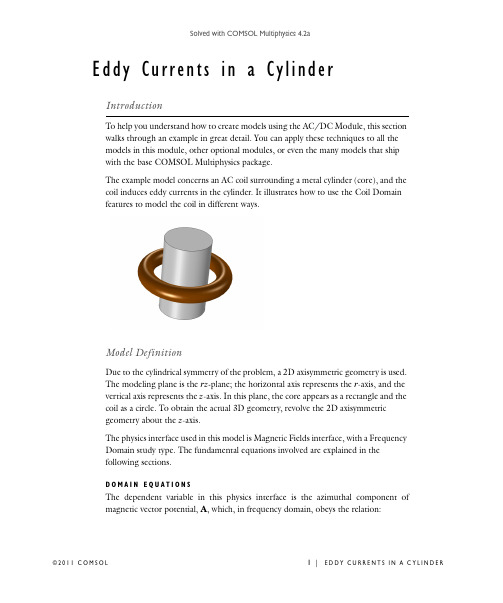
Eddy Currents in a CylinderIntroductionTo help you understand how to create models using the AC/DC Module, this section walks through an example in great detail. You can apply these techniques to all the models in this module, other optional modules, or even the many models that ship with the base COMSOL Multiphysics package.The example model concerns an AC coil surrounding a metal cylinder (core), and the coil induces eddy currents in the cylinder. It illustrates how to use the Coil Domain features to model the coil in different ways.Model DefinitionDue to the cylindrical symmetry of the problem, a 2D axisymmetric geometry is used.The modeling plane is the rz-plane; the horizontal axis represents the r-axis, and the vertical axis represents the z-axis. In this plane, the core appears as a rectangle and the coil as a circle. To obtain the actual 3D geometry, revolve the 2D axisymmetricgeometry about the z-axis.The physics interface used in this model is Magnetic Fields interface, with a Frequency Domain study type. The fundamental equations involved are explained in thefollowing sections.D O M A I NE Q U A T I O N SThe dependent va ria ble in this physics interfa ce is the a zimutha l component of magnetic vector potential, A, which, in frequency domain, obeys the relation:(1)where ω is the angular frequency, σ is the electric conductivity, μ is the permeability, εis the permittivity, and denotes the current density due to an external source. One wa y to define the current source is to specify a distributed current density in the right-hand side of the above equation. This current density gives rise to a current I as defined by:(2)B O U N D A R YC O ND I T I O N SThis model requires boundary conditions for the exterior boundary and the symmetry xis, a nd to specify bounda ry currents when a pplica ble. The physics interfa ce a utoma tica lly a pplies a bounda ry condition corresponding to zero ma gnetic flux through the exterior bounda ry, by setting the vector potentia l to zero. On the symmetry axis, a suitable symmetry boundary condition is applied.C O I L G R O U PD O M A I N SThe Magnetic Fields interface provides features, called Coil Group Domain, that can conveniently be used to model coils in 2D and 2D axisymmetric geometries.The Single-Turn Coil Domain models a single winding of a homogeneous metallic conductor, in which the current density ca n be non-uniform, due to the a xia l symmetry or skin effect. Note that applying the Single-Turn Coil Domain feature to multiple domains effectively consists in having multiple coils in parallel.The Multi-Turn Coil Domain is used to model a great number of tiny wires wound together. In this approximation, the current density is uniform, and no conduction currents appear in the domain. From this follows that the material used to model this domain should reflect the properties of the insulator covering the wires, rather than of the metal constituting the windings.A third Coil Doma in fea ture is provided, tha t is not used in this model. The Coil Group Doma in fea ture is identica l to the Single-Turn Coil Doma in, with the importa nt difference tha t a pplying this fea ture to multiple doma ins connects the resulting coils in series.j ωσω2ε–()A ϕ∇μ1–∇A ϕ×()×+J ϕe =J ϕe J e d s ⋅S ∫I =Results and DiscussionThe eddy currents induced in the cylinder are shown in the following figures. The induced currents on the cylinder are of comparable magnitude, due to the choice of the parameter, but the current density in the coil is different. Figure 1 presents the results obtained with a Single-Turn Coil Domain feature. The current density is not uniform and is greater in the inner part of the coil (the region closer to the z axis) and close to the surface (due to the skin effect).Figure 1: Results using a Single-Turn Coil Domain feature.In Figure 2, the Multi-Turn Coil Domain feature is used. While the effect on the cylinder is similar to the one obtained with a Single Turn Coil Domain, the current density in the coil is uniform, according to the coil approximation stated above.Figure 2: Results using a Multi-Turn Coil Domain feature.Model Library path: ACDC_Module/Tutorial_Models/coil_eddy_currentsThe Model Library path shows the location of the Model MPH-file. You can open it directly from the Model Library (accessible from the View menu) and browsing to ACDC Module>Tutorial Models>coil eddy currents.Modeling InstructionsM O D E L W I Z A R D1Go to the Model Wizard window.2Click the 2D axisymmetric button.3Click Next.4In the Add physics tree, select AC/DC>Magnetic Fields (mf).5Click Add Selected.6Click Next.7Find the Studies subsection. In the tree, select Preset Studies>Frequency Domain.8Click Finish.G E O M E T R Y1The following instructions explain how to build the model geometry.Rectangle 11In the Model Builder window, right-click Model 1>Geometry 1 and choose Rectangle. 2Go to the Settings window for Rectangle.3Locate the Size section. In the Width edit field, type 0.2.4In the Height edit field, type 0.5.5Locate the Position section. In the z edit field, type -0.25.6Click the Build Selected button.Rectangle 21In the Model Builder window, right-click Geometry 1 and choose Rectangle.2Go to the Settings window for Rectangle.3Locate the Size section. In the Width edit field, type 0.03.4In the Height edit field, type 0.1.5Locate the Position section. In the z edit field, type -0.05.6Click the Build Selected button.Circle 11In the Model Builder window, right-click Geometry 1 and choose Circle.2Go to the Settings window for Circle.3Locate the Size and Shape section. In the Radius edit field, type 0.01.4Locate the Position section. In the r edit field, type 0.05.5Click the Build All button.6Click the Zoom Extents button on the Graphics toolbar.This concludes the construction of the geometry. The next step is the definition of the material properties. Define the materials constituiting the coil and the core.M A T E R I A L SMaterial 11In the Model Builder window, right-click Model 1>Materials and choose Material.2Select Domain 3 only.3Go to the Settings window for Material.4Locate the Material Contents section. In the Material contents table, enter the following settings:PROPERTY NAME VALUEElectrical conductivity sigma 3.7e7[S/m]Relative permittivity epsilonr1Relative permeability mur15Right-click Material 1 and choose Rename.6Go to the Rename Material dialog box and type Coil in the New name edit field.7Click OK.Material 21Right-click Materials and choose Material.2Select Domain 2 only.3Go to the Settings window for Material.4Locate the Material Contents section. In the Material contents table, enter the following settings:PROPERTY NAME VALUEElectrical conductivity sigma 3.7e7[S/m]Relative permittivity epsilonr1Relative permeability mur15Right-click Material 2 and choose Rename.6Go to the Rename Material dialog box and type Core in the New name edit field.7Click OK.Material BrowserThe third material needed for the model is Air, used for the domain surrounding the core and the coil. The material parameters for air are already available in COMSOL Multiphysics, and can be accessed using the Material Browser.8Right-click Materials and choose Open Material Browser.9Go to the Material Browser window.10Locate the Materials section. In the Materials tree, select Built-In>Air.11Right-click and choose Add Material to Model from the menu.Air1In the Model Builder window, click Air.2Select Domain 1 only.M A G N E T I C F I E L D SThe next step consists in setting up of the physics interface. The Magnetic Fields interface automatically provides default domain and boundary conditions. Thefollowing instructions explain how to apply a current density using a Single-Turn Coil Domain feature.Single-Turn Coil Domain 11In the Model Builder window, right-click Magnetic Fields and choose Single-Turn Coil Domain.2Select Domain 3 only.3Go to the Settings window for Single-Turn Coil Domain.4Locate the Single-Turn Coil Domain section. In the I coil edit field, type 1[kA].No further actions are required in the physics interface. The next step is the mesh generation. To better resolve the induced current density in the core and the coil, choose Fine as the mesh size.M E S H11In the Model Builder window, click Model 1>Mesh 1.2Go to the Settings window for Mesh.3Locate the Mesh Settings section. From the Element size list, choose Fine.4Click the Build All button.S T U D Y1The last step consists in setting up the study. An operating frequency must be provided in the Frequency Domain study.Step 1: Frequency Domain1In the Model Builder window, click Study 1>Step 1: Frequency Domain.2Go to the Settings window for Frequency Domain.3Locate the Study Settings section. In the Frequencies edit field, type 100[Hz].4In the Model Builder window, right-click Study 1 and choose Compute.R E S U L T SWhen the solution process is completed, a default plot is generated, showing the norm of the magnetic flux density. Additional plots can be added to visualize other quantities. The following instructions illustrate how to plot the current density and the streamlines of the magnetic flux density.2D Plot Group 21In the Model Builder window, right-click Results and choose 2D Plot Group.2Right-click Results>2D Plot Group 2 and choose Surface.3Go to the Settings window for Surface.4In the upper-right corner of the Expression section, click Replace Expression.5From the menu, choose Magnetic Fields>Currents and charge>Current density>Current density, phi component (mf.Jphi).6In the Model Builder window, right-click 2D Plot Group 2 and choose Streamline.7Go to the Settings window for Streamline.8Locate the Streamline Positioning section. From the Positioning list, choose Start point controlled.9In the Points edit field, type 15.10In the upper-right corner of the Expression section, click Replace Expression.11From the menu, choose Magnetic Fields>Magnetic>Magnetic flux density (mf.Br,mf.Bz).12Locate the Coloring and Style section. From the Color list, choose Red.13Click the Plot button.14Click the Zoom In button on the Graphics toolbar.The plot shows the azimuthal current density in the core and in the coil. The current density in the coil is greater in the inner part, and due to the skin effect, is more concentrated at the surface.The next instructions illustrate how to modify the model in order to use a Multi-Turn Coil Domain for the excitation. The first step is to change the material model to an insulator. In this case, Air can be used.M A T E R I A L SAir1In the Model Builder window, click Model 1>Materials>Air.2Select Domains 1 and 3 only.Before adding a Multi-Turn Coil Domain feature, the Single-Turn Coil Domain must be disabled.M A G N E T I C F I E L D SSingle-Turn Coil Domain 1In the Model Builder window, right-click Model 1>Magnetic Fields>Single-Turn CoilDomain 1 and choose Disable.Multi-Turn Coil Domain 11Right-click Magnetic Fields and choose Multi-Turn Coil Domain.2Select Domain 3 only.Specify the conductivity of the metal constituting the coil wires.3Go to the Settings window for Multi-Turn Coil Domain.4Locate the Multi-Turn Coil Domain section. In the σcoil edit field, type 3e7[S/m].To obtain comparable effects on the core, set the number of windings to 1000 andapply a current of 1 A.5In the N edit field, type 1000.6In the I coil edit field, type 1[A].S T U D Y11In the Model Builder window, right-click Study 1 and choose Compute.R E S U L T SAfter the solution process, update the plot group to visualize the new results.2D Plot Group 21In the Model Builder window, right-click Results>2D Plot Group 2 and choose Plot.2Click the Zoom Extents button on the Graphics toolbar.©2011C O M S O L11|E D D Y C U R R E N T S I N A C Y L I N D E R3Click the Zoom In button on the Graphics toolbar.The induced current density in the core is comparable to the previous case; thecurrent density in the coil, instead, is uniform.12|E D D Y C U R R E N T S I N A C Y L I N D E R©2011C O M S O L。