TSic应用笔记
tsne用法

t-SNE是一种高效的数据可视化技术,可用于降维和可视化高维空间数据,如图像和多维标识符。
下面将介绍t-SNE的工作原理和使用方法。
1. t-SNE是什么?
t-SNE代表t分布随机近似嵌入,它是一种非线性降维技术。
可以将高维数据集映射到低维空间,以便更容易可视化和理解数据。
2. t-SNE的工作原理
t-SNE通过最小化高维空间中点之间的距离来确定低维表示,同时最小化该距离与点的相似性分布之间的误差。
它使用了一种称为T分布的概率分布,以保持相似性分布的局部不变性。
3. 如何使用t-SNE进行数据可视化?
要使用t-SNE对数据进行可视化,您需要将数据准备好:构建一个特征矩阵,并确定您要显示的数据点的标签。
然后,将数据传递给t-SNE算法,该算法将执行降维操作并返回一组低维数据点。
4. t-SNE的优缺点
与其他降维技术相比,t-SNE具有更好的可视化效果和良好的局部不变性。
缺点是计算量较大,并且降维过程不可逆。
5. t-SNE的应用领域
t-SNE已经成功地应用于图像识别、自然语言处理、信号处理和计算机视觉等领域。
它肘可以帮助研究人员更好地理解他们的数据,发现数据中的模式和关系。
总之,t-SNE是一种非常有用的数据可视化技术,它为研究人员提供了一个强大的工具,可以探索和可视化高维空间数据。
学习笔记-USIM卡规范全解
1什么是UICC卡UICC-- Universal Integrated Circuit Card通用集成电路卡是定义了物理特性的智能卡的总称。
作为3G用户终端的一个重要的、可移动的组成部分,UICC主要用于存储用户信息、鉴权密钥、短消、付费方式等信息,还可以包括多种逻辑应用,例如用户标识模块(SIM)、通用用户标识模块(USIM)、IP多媒体业务标识模块(ISIM),以及其他如电子签名认证、电子钱包等非电信应用模块。
UICC 中的逻辑模块可以单独存在,也可以多个同时存在。
不同的3G用户终端可以根据无线接入网络的类型,来选择使用相应的逻辑模块。
在3G用户终端的入网测试中,要求满足UICC的一致性测试要求。
UICC的一致性测试包括物理特性、电气特性和传输协议测试等几个方面,其中传输协议测试涉及到对UICC 的文件访问和安全操作。
ISO/IEC国际化标准组织制定了一系列的智能卡安全特性协议,以确保3G用户终端对UICC文件的安全访问。
2USIM卡与SIM卡的比较USIM卡和SIM卡相比有如下特点:◆相对于SIM卡的单向鉴权(网络鉴权用户),USIM卡鉴权机制采用双向鉴权(除了网络鉴权用户外,用户也鉴权网络),有很高的安全性。
◆于SIM卡电话薄相比,USIM卡电话薄中每个联系人可以对应多个号码或者昵称。
◆相对SIM卡机卡接口速率,USIM卡机卡接口速率大大提高(230kbps)。
◆相对SIM卡对逻辑应用的支持,USIM可以同时支持4个并发逻辑应用。
SIM卡的上下电过程上电过程:RST低电平状态->Vcc加电->I/O口处于接收状态->Vpp加电->提供稳定的时钟信号。
关闭过程:RST低电平状态->CLK低电平状态->Vpp去电->I/O口低电平状态->Vcc去电GSM网络注册过程中用到的对SIM卡的操作:1. 手机开机后,从SIM卡中读取IMSI(15Digits)和TMSI(4byte);2. 手机把IMSI或TMSI发送给网络;3. 网络检验IMSI或TMSI有效,生成一个128bit的RAND发送给手机。
AD536ADJ真有效值交流转换直流IC的研究与应用

AD536ADJ真有效值交流转换直流IC的研究与应用首先,我们来了解一下AD536ADJ的基本特性和工作原理。
AD536ADJ是一款基于电荷平衡原理的电压转换器,可以将直流输入信号转换为等效的交流输出信号。
它内部集成了一个内部振荡器和一个电荷积分放大器,可以实现高精度和高稳定性的转换功能。
AD536ADJ的主要特性包括:输入电压范围广,可接受0V至40V的直流输入;输出频率范围宽,可以达到1Hz至100kHz;转换精度高,可达到0.1%;工作温度范围广,可以在-40℃至85℃的环境下正常工作。
在实际应用中,AD536ADJ有着广泛的用途。
首先,它可以用于电源管理领域。
电源管理是指对电源电压进行监测和控制,以提供稳定和可靠的电源输出。
AD536ADJ可以通过将直流电源转换为交流信号,实现对电源电压的实时监测和控制。
在电力系统中,可以将AD536ADJ与其他电源管理器件配合使用,实现对功率因数、电压波形和电源负载的控制。
其次,AD536ADJ还可以应用于工业自动化控制领域。
工业自动化控制是指通过自动化设备和技术,实现对工业生产过程的监控和控制。
AD536ADJ可以作为工业自动化控制系统中的一个重要组成部分,用于检测和控制过程中的直流信号。
例如,在温度控制系统中,AD536ADJ可以将温度传感器的直流信号转换为交流信号,再经过控制器进行处理和控制。
此外,AD536ADJ还可以应用于测量和仪器领域。
在科学实验和工程测量中,常需要将直流信号转换为交流信号进行测量和分析。
AD536ADJ可以实现高精度和高稳定度的直流转交流转换,提供精确的测量结果。
总之,AD536ADJ作为一款高性能的直流转交换电压转换器集成电路,具有广泛的研究和应用价值。
它可以在电源管理、电力系统和工业自动化控制等领域发挥重要作用,实现对直流信号的高精度和高稳定度的转换。
相信随着科技的不断进步,AD536ADJ的研究和应用将会有更加广阔的前景。
电容应用分析精粹:从充放电到高速PCB设计

第16章施密特 2
触发器构成的 多谐振荡器
3 第17章电容器
的串联及其应 用
4 第18章电容器
的并联及其应 用
5 第19章电源滤
波电路基本原 理
第21章从电容充放 电认识低通滤波器
第20章从低通滤波 器认识电源滤波电
路
第22电容的容量 越大越好吗
第32章旁路电容工作 原理(模拟电路)
第33章旁路电容与去 耦电容的与区别
第34章旁路电容中的 战斗机:陶瓷电容
第35章交流信号是如 何通过耦合电容的
第36章为什么使用电 容进行信号的耦合
第37章耦合电容的容 量多大才合适
第38章 RC超前型移 相式振荡电路
第39章超前滞后相移 应用:RC文氏电桥
电路的复位应 用
5 第9章门电路组
成的积分型单 稳态触发器
第10章 555定 时芯片应用:
1
单稳态负边沿
触发器
第11章 RC多 2
谐振荡器电路 工作原理
3 第12章这个微
分电路是冒牌 的吗
4 第13章门电路
组成的微分型
单稳态触发器
5
第14章 555定 时器芯片应用:
单稳态正边沿
触发器
第15章电容器 1
0 2
第47章使 用加速电容 优化开关电 路的速度
0 3
第48章密 勒电容对电 路高频特性 的影响
0 4
第49章功 放与开关电 源中的自举 电容
0 6
反侵权盗版 声明
0 5
第50章安 规电容工作 原理及应用
作者介绍
这是《电容应用分析精粹:从充放电到高速PCB设计》的读书笔记模板,暂无该书作者的介绍。
IC原理与应用-离子色谱法

6
4 2 0 20 25 30 35 40 45
F-
温度, ℃
流速的影响
SO4212000
HPO42NO3-
流速增加
峰面积
10000 8000
BrNO2-
溶质峰面积 减小
Cl6000 4000 2000 0 0.5 1 1.5 2
F-
流速(mL/min)
流动相组成的影响
20 保留时间 (min)
5.0 ppm 8.6 8.7 8.8 8.9 8.9 9.1
0
4
8 12 保留时间 (min)
16
抑制器的作用
淋洗液 (Na2CO3) - , SO - 2 样品 F , CI 4 不经过抑制 对离子 F分析柱 mS CI SO42 -
废液 阴离子抑制 H2O 器
H+
Na+ OH-
NaF, NaCl, Na2SO4 in Na2CO3 废液 H2 O mS
20
离子对色谱分离原理
H 2O
(TBA+X-) ACN TBA+OHACN (TBA+X-) ACN TBA+OHACN (TBA+X-) ACN
ACN
+
Y+ X-
流动相
TBAOH/ACN/H2O
TBA OH (TBA+X-)
样品
Y+ X Y+ OH-
固定相
TBA+ OHY+ XACN
H 2O
疏水
16 12 8 4 0 0 0.11 0.22 0.33 SO42HPO42NO3BrNO2ClF-
基本原理:离子色谱中发生的基本过程就是离
李瀚荪《电路分析基础》笔记和典型题(含考研真题)详解(集总参数电路中电压、电流的约束关系)
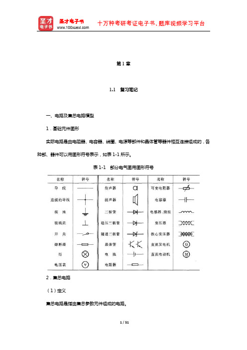
第1章1.1 复习笔记一、电路及集总电路模型1.基础元件图形实际电路是由电阻器、电容器、线圈、电源等部件和晶体管等器件相互连接组成的,各种部、器件可以用图形符号表示,如表1-1所示。
表1-1 部分电气图用图形符号2.集总电路(1)定义集总电路是指由集总参数元件组成的电路。
(2)应用条件当电路的尺寸远小于最高频率所对应的波长时,可以当做集总电路来处理。
二、电路变量电流、电压及功率1.电流(1)定义电流是指每单位时间内通过导体横截面的电荷量。
(2)表达式电流的表达式为(3)分类①恒定电流恒定电流是指大小和方向都不随时间变化的电流,简称直流。
②交变电流交变电流是指大小和方向都随时间作周期性变化的电流,简称交流。
2.电压(1)定义电路中a、b两点间的电压是指单位正电荷由a点转移到b点时所获得或失去的能量。
(2)表达式电压的表达式为(3)分类①恒定电压恒定电压是指大小和极性都不随时间而变动的电压,也叫直流电压。
②时变电压时变电压是指大小和极性都随时间变化的电压,也叫交流电压。
(4)关联参考方向:关联参考方向是指电流参考方向与电压参考方向一致,如图1-1所示。
图1-1 关联的参考方向3.功率(1)定义功率是指能量流动的速率。
(2)表达式功率的表达式为p(t)=u(t)i(t)(3)功率的正负功率的正负表示能力的吸收与产生,电压电流取关联参考方向时:①当功率为正,电路吸收能量,p值即为吸收能量的速率;②当功率为负,电路提供能量,p值为产生能量的速率。
三、基尔霍夫定律1.基尔霍夫电流定律(1)定律内容基尔霍夫电流定律可表述为:对于任一集总电路中的任一节点,在任一时刻,流出(或流进)该节点的所有支路电流的代数和为零。
(2)表达式基尔霍夫电流定律的数学表示式为(3)理论基础基尔霍夫电流定律的理论基础是电荷守恒法。
2.基尔霍夫电压定律(1)定律内容基尔霍夫电压定律可表述为:对于任一集总电路中的任一回路,在任一时刻,沿着该回路的所有支路电压降的代数和为零。
micrel麦瑞以太网产品应用笔记
应用笔记120无变压器以太网连接的电容耦合麦瑞10/100 以太网产品简介PHY 连接不使用变压器的电容耦合连接方式是减BOM 成本和PCB 面积的常用方式。
本应用笔记描述了麦瑞 10/100 以太网器件电容耦合的方法。
麦瑞器件的电容耦合KS8695X CENTAUR -集成多端口网关方案。
KS8695P/PX CENTAUR -集成多端口PCI 网关案。
KS8721B/BT 单个10/100 PHY 端口,不带MDI/MDI-X 自动切换接口KS8721BL/SL 3.3V 单电源供电10/100PHY 带MDI/MDI-X 自动切换接口KS89933端口10/100 无管理交换机KS8993F 3端口10/100 管理/无管理交换机/媒体转换器。
KS8993M 3端口10/100管理/无管理交换机。
KS8995M/X 5端口10/100管理/无管理交换机。
KS8995MA/XA 5端口10/100管理/无管理交换机。
KS89978端口10/100无管理交换机。
KS89998端口10/100无管理交换机。
电容耦合方法电容耦合的方法取决于接收电路是否提供了内部DC 偏置补偿。
传输端图1和图2显示了传输端的电容耦合方式。
在这个方法中,50欧的上拉电阻R1和R2被上拉至模拟电源VDD 。
除了器件KS8993外,所有在本应用笔记列出的麦瑞器件都需要这个终端输出。
对于KS8993,R1和R2是连接在一起,但是不是连接到VDD ,差分信号TXPx 和TXMx 每个断点上拉50欧的电阻到引脚VERF 。
带内部DC 偏置的器件的接收端图1 显示了电容耦合到一个带有内部DC 偏置的接收端的电路图。
50欧的上拉电阻R3和R4成对的连接到C3,然后连接到模拟电源VDD ,用以提供正确的接收输入端。
这个方法可以应用于KS8993,因为它提供了内部DC 偏置。
图1 带有内部DC 偏置的接收端的电容耦合电路不带内部DC 偏置的器件的接收端图2显示了电容耦合到一个带有内部DC 偏置的接收端的电路图。
ST AN1089 应用笔记
INTRODUCTIONPFC preregulators based on the boost topology working in Transition Mode (TM, see fig. 1) have been widespread in electronic lamp ballast systems. This kind of equipment almost always works under a sin-gle mains supply (110 or 220 VAC, with some tolerance) and the use of a PFC preregulator is mainly aimed at optimising the downstream half-bridge lamp driver and improving their inherent extremely poor PF.The PFC preregulator sees the downstream stage as a constant load, so it is requested to work under a limited range of operating conditions. From the control loop standpoint, this means that the frequency compensation of the error amplifier can be very simple, typically just a feedback capacitor. Its capaci-tance will be high enough to ensure the crossover frequency of the open loop gain is low, so as to achieve a high PF (see Ref. [1]).March 2000®AN1089APPLICATION NOTECONTROL LOOP MODELING OF L6561-BASED TM PFCby Claudio AdragnaThis paper provides a model and a tool for evaluating and improving the control loop characteristics of L6561-based PFC preregulators in boost topology and operated in Transition Mode (TM).Such a subject is now becoming topical since TM PFC preregulators are more and more used in sys-tems other than electronic lamp ballast where the input voltage range is limited and the load current is almost constant.The ability to operate under large variations of both input voltage and load current, as well as the use of TM PFC systems as preregulators for switching converters, requires a more accurate design of the control loop. The goal will be not only to ensure a narrow bandwidth in order to achieve a high Power Factor, but also to have enough phase margin so as to make sure the system is stable over a large range of operating conditions.83R9R10Vac56L6561721R7CoRsR8+-4VccVoCompensation NetworkFigure 1. Typical L6561-based TM PFC preregulator1/12Things get more complicated when an electronic ballast can supply two lamps and is required to work even if one lamp is not used or is exhausted, so that it is expected to work at half load as well.The L6561, thanks to its highly linear, wide dynamics multiplier, extends the use of TM PFC boost pre-regulators to applications that experience a wide range of operating conditions, both in terms of input voltage variations and load change. High power (60 to70 W) AC-DC adapters for portable equipment and computer monitor SMPS’ are the most noticeable examples.This, however, calls for a more accurate design of the control loop than the one illustrated in Ref.[1]. The control goal will no longer be to achieve only a low crossover frequency but also an adequate phase margin. Besides ensuring stability over a large variety of operating conditions, this is necessary to pre-vent dangerous oscillations of the output voltage as a result of load changes.PFC Boost Preregulator Control LoopTo the aim of finding a compensation network able to achieve the above mentioned control goal, it is necessary to get an insight into the control loop of such systems. This can be synthesised as shown in the block diagram of fig. 2.VirmsERROR AMPLIFIER G1(s)MULTIPLIERG2PWM MODULATORPOWER STAGEG4(s)FEEDBACKHG3+ -+ -ZCDVrefVoV COMPV cspkI LpkFigure 2. Control loop of a PFC Preregulator: Block Diagram-+DRIVER-+PWMCOMPARATORRsE/A VREF (2.5V)L6561VoV REFLDCo7124Q3RQ5SMULTIPLIER ZCDSTARTERE/ACOMPENSATION NETWORKINVCOMPMULT CS ZCDGDG4(s)G3HG1(s)G2K P · ViV csViV COMPR7R8R9R10V csFigure 3. Control loop of a PFC Preregulator: electrical circuit and main quantitiesFig. 3 illustrates how the various blocks of fig. 2 relate with the electrical circuit, both external and inside the L6561. For details on the internal circuit and its operation please refer to Ref. [1].The loop gain of PFC preregulators must have a very low crossover frequency (fc) so as to maintain V COMP (Error Amplifier output) fairly constant over a given line cycle and ensure a high PF. As a rule of thumb, fc should not exceed 20-25 Hz at maximum mains voltage.This allows to assume that the control action takes place on the peak amplitude (or, which is the same,the RMS value) of the various quantities inside the loop.The first step is to determine the transfer function of the power stage, G4(s), defined as:G4(s ) =dV o dI Lpk = dV o dI o ⋅dI odI Lpkwhere Vo is the DC output voltage, Io the DC output current and I Lpk is the peak value of the inductor cur-rent.Under the above assumption, the power stage can be modeled as illustrated in fig. 4: a controlled cur-rent source (with a shunt resistor Re) that drives the output bulk capacitor Co and the load resistance Ro (= Vo / Io). The zero due to the ESR associated with Co is far beyond the crossover frequency thus it is neglected.The current source can be characterised with the fol-lowing considerations: the low frequency component of the boost diode current is found by averaging the discharge portion of the inductor current (the white triangles of fig. 5) over a given switching cycle.The low frequency current, averaged over a mains half-cycle yields the DC output current Io:I o = 12 ⋅ (1 − D ) ⋅ I Lpk ⋅ sin θ_________________ = 12 ⋅√ 2 ⋅ V irms ⋅ sin θ ⋅ I Lpk ⋅ sin θ_________________________V o= √ 24 ⋅ V irms ⋅ I Lpk V o where D is the switch duty cycle, θ is the in-stantaneous phase angle of the mains volt-age and V irms its effective (RMS) value.The AC model illustrated in fig. 4 can be found by calculating the total differential of the above expression of Io. A few algebraic manipulations would show that the shunt re-sistor Re always equals the DC load resis-tance Ro, thus it changes depending on the power delivered by the system. Now it is necessary to consider two separate cases.If the load is purely resistive (or equivalent to a resistor, like in the case of a lamp ballast circuit), the AC load resistance equals Ro.The parallel of this resistance with Re, com-bined with the output bulk capacitor, gives origin to a pole located at:ωp =2R o ⋅ C owhich is usually in the range of 1 to 5 Hz.Co RoRe IoVoFigure 4. Power stage model,G4(s)Inductor current peak envelopeLow frequency Diode currentON OFFSWITCHDiode current Switch currentI LpkIoFigure 5. Boost PFC currentsIn case the PFC preregulator provides a DC bus supplying a downstream switching converter, the load should be regarded as a "constant power" load rather than a resistor. In fact, as long as a switching con-verter is in regulation, the power it demands of the source is practically independent of the input voltage (converter’s efficiency changes very little).In this case, the AC load resistance is equal to -Ro (if the DC bus decreases the current demanded of the PFC increases, whence the negative sign). As a result, the parallel combination with Re tends to in-finity and the two resistances cancel. The current source drives only the output capacitor and the pole lo-cation tends to zero. In the end, G4(s) will be given by:G4(s ) =√ 28 ⋅ V irms V o ⋅ R o1 + s ⋅R o ⋅ C o2(resistive load ) √ 24 ⋅V irms V o ⋅ 1s ⋅C o (constant power load ) .The gain of the PWM modulator, G3, which includes the current loop, is simply:G3 =dI Lpk dV cspk = 1R swhere R s is the sense resistor connected be-tween the source of the external MOSFET and ground (across which the L6561 reads the induc-tor current through pin 3).To calculate the transfer function G2 of the multi-plier block, one can consider that a variation ∆V COMP , due to a line and/or load change, modi-fies the peak amplitude Vcspk of the rectified sinusoid at the output of the multiplier.Therefore:G2 =dV cspkdV COMP= K M ⋅ K P ⋅ √ 2⋅ V irmswhere K M is the gain of the multiplier and K P the partition ratio of the resistor divider that feeds a portion of the input voltage into pin 3.The electrical characteristics of the L6561 specify K M = 0.6 ±25% (@V COMP = 4V, including temperature)but actually K M decreases for low values of V COMP . In fig. 6 the typical value of K M is plotted against V COMP along with the tolerance limits. Since V COMP gets lower when the mains voltage is high, this vari-ation of K M partly compensates for the increase of G2 with V irms , thus providing a mild voltage feedfor-ward effect.If one wants to take this non-linearity into account, he or she should linearise the large-signal multiplier gain in the neighborhood of the quiescent point of the error amplifier, so as to get the small-signal gain (km). Please refer to [1] and the Appendix for the relevant calculation technique.Ultimately, the control-to-output transfer function will be:G (s ) = dV O dV COMP = G2 ⋅ G3 ⋅ G4(s ) = 14 ⋅ km ⋅ K P ⋅ V 2irms V O ⋅ R o R s ⋅ 11 + s ⋅R O ⋅ C O 2(resistive load )12 ⋅km ⋅ K P ⋅ V 2irmsR s ⋅ V O ⋅ 1s ⋅ C O (constant power load )where the small-signal multiplier gain km could be assumed equal to K M for simplicity.2.533.54 4.555.50.10.20.30.40.50.60.70.80.9VCOMPKMFigure 6. Plot of K M vs. E/A outputFrom the above equations, it is apparent that the gain of the control-to-output function is strongly dependent on the input voltage, despite the slight compensation provided by K M . For design purpose, G(s) will have to be considered at the maximum mains voltage, where the gain is maximum and the loop bandwidth is maxi-mum as well.The feedback block is usually made up of a simple resistor divider (see fig. 7). Only the upper resistor R7is significant to the loop gain (the lower resistor R8just sets the value of Vo). It is then convenient to as-sume H=1 and to consider R7 as a part of the error amplifier block G1(s).Error Amplifier CompensationIn PFC preregulators that supply an electronic lamp ballast the error amplifier is compensated typically as shown in fig. 7 (see also Ref. [2] and [3]).For this kind of load this circuit gives satisfactory results. It may not be acceptable, however, in other systems where stability must be ensured over a wide range of input voltage and load current, and does not work at all when the PFC preregulator supplies a switching converter.Figure 8 shows the suggested compensation schemes for both the cases under consideration.With a resistive load the loop can be stabilised by adding a pole in the origin plus a low frequency zero that compensates the pole of the control-to-output gain (network a). Ideally, this can give the desired bandwidth with 90° phase margin as well as high DC gain for good load regulation.With a constant power load the control-to-output gain has a pole in the origin thus the DC gain of the er-ror amplifier should be externally limited with a feedback resistor. If not, a second pole in the origin would be introduced, which would result in a system whose stability might be critical.Limiting the gain goes to the detriment of preregulator’s load regulation but this has not a serious impact on the overall system since the downstream converter will easily compensate for that.The compensation network (b) adds a pole-zero couple that both makes the gain roll off at low frequency (so as to cross the 0 dB axis at low frequency) and boosts the phase in the neighborhood of the cross-over frequency (so as to increase phase margin).The transfer functions of the compensation networks of fig. 8 a) and b) are respectively:G1(s ) =dV COMP dV O = 1 + s ⋅ C3 ⋅ R11s ⋅ C3 ⋅ R7(circuit a − resistive load )R12R7 ⋅ 1 + s ⋅ C3 ⋅ R111 + s ⋅ C3 ⋅ (R11 + R12)(circuit b − constant power load )INV2.5VE/A +_L6561C3R7TO MULTIPLIER21R8V oFigure 7. Typical compensation scheme inPFC preregulators for lamp ballastCOMPINV2.5VE/A +_L6561C3R12R7TO MUL TIPLIERR1121R8VoCOMPINV2.5VE/A +_L6561C3R7TO MUL TIPLIERR1121R8Voa) resistive load b) constant power loadFigure 8. Suggested compensation networks for TM boost PFCAs a tool to ease the design of L6561’s E/A compensation networks in TM boost PFC preregulators, the Appendix contains a Mathcad® file gathering the theory above illustrated and performing all the neces-sary calculations.ConclusionsThis paper gets an insight into the control loop of TM controlled Boost PFC preregulators based on the L6561 PFC controller. This reveals that the simple feedback capacitor used to compensate the error am-plifier in preregulators for lamp ballast may not be adequate in systems that may experience large vari-ations in input voltage and/or load current. Moreover it leads to an unstable loop if the load is a switching converter. Appropriate compensation schemes are suggested for both cases and a calculation tool (Mathcad® file) is provided so as to make control loop design easier in such systems.References[1] "L6561, Enhanced Transition Mode Power Factor Corrector", (AN966)[2] "L6569 - L6561 Lighting Application with PFC" (AN991)[3] "Electronic Ballast with PFC Using L6574 and L6561" (AN993)[4] "Design Equations of High-Power-Factor Flyback Converters Based on the L6561" (AN1059)[5] "Flyback Converters with the L6561 PFC Controller" (AN1060)AppendixThis Mathcad® file allows to design the control loop and performs a stability analysis of PFC preregula-tors in boost topology operated in Transition Mode and controlled by the L6561.Highlighted equations indicate data that must be manually entered. These data are supposted to be known to the user as a result of the design of the PFC preregulator (the use of the PFC design software included in the CD-ROM "Linear and Switching Voltage Regulators" is recommended). The example val-ues are taken from the L6561 demo board circuit.PFC Converter Data:Output Voltage V O := 400VOutput Capacitor C O := 47µFSense Resistor R s := 0.41ΩOutput Overvoltage Threshold OVP := 40V Expected Efficiencyη := 0.9Multiplier Biasing:Input Divider Upper Resistor R up := 1240kΩInput Divider Lower Resistor R low := 10kΩAnalysis Setpoint:Mains RMS Voltage V irms := 264VOutput Power P O := 80WPreliminary calculations & Service Variables:Equivalent Load ResistanceR o :=V O 2P OR O = 2 ⋅103ΩInput Divider GainKP :=R lowR low + R upKP = 8 ⋅10-3Large-signal Multiplier Gain:KM(V COMP ) := 0.651 ⋅ (1 - 85.29 ⋅ e -1.776 ⋅ VCOMP )Error Amplifier Quiescent Point:V COMP := 4V COMP := root2.5 +2 ⋅ P o ⋅ R Sη ⋅ KM (V COMP ) ⋅ KP ⋅ V irms 2 − V COMP , V COMPV COMP = 2.898 [V]Small signal Multiplier Gainkm :=ddV COMP[KM (V COMP ) ⋅ (V COMP − 2.5)]km = 0.557------------------------------------------------------------------------------------------------------------------------------------------j: = √ -1 n: = 100 Dec: = 6 w:= 0,1..n ω(w): = 10w ⋅ Decn− 1f: = 1Control-to-Output Transfer Function (constant power load):G (ω) : = km ⋅ KP ⋅ V irms 22 ⋅ V O⋅ 1R S ⋅106j ⋅ ω ⋅ C O Compensated E/A Transfer Function (constant power load, refer to fig.8b)DC gain (∆V O /∆V COMP ):G O := 0.30Pole:p := 0.23Hz Zero:z := 15Hz0.11101001.10350050100150¦G¦fd B0.11101001.103919089/Gfd e gTransfer Function:G1(ω) := G O ⋅ 1 + j ⋅ω2 ⋅ π ⋅ z1 + j ⋅ω2 ⋅ π ⋅ pOpen Loop Transfer Function (constant power load):F(ω): = G (ω) ⋅ G1 (ω)ΦF(ω): = arg (F(ω)) ⋅180πCrossover Frequency:fc: = |root (|F(2 ⋅ π ⋅ f)| - 1, f)|fc = 18.836HzPhase Margin:Φ : = 180 + ΦF (2 ⋅ π ⋅ fc)Φ = 52.167°0.11101001.1036040200¦G1¦fd B0.11101001.103100806040200/G1fd e g0.11101001.103100100¦F¦fd B0.11101001.10320016012080400/Ffd e gFeedback Network Implementation (constant power load, refer to fig. 8b):Output Divider Upper Resistor R7: =OVP40⋅ 103 R7 = 1 ⋅ 103k ΩOutput Divider Lower Resistor R8: = 2.5V O − 2.5 ⋅ R7 R8 = 6.289k ΩParallel Feedback Resistor:R12: = G O ⋅ R7 R12 = 300k ΩSeries Feedback CapacitorC3: = 1062 ⋅ π ⋅ R12 ⋅ 1p ⋅ 1zC3 = 2.271 ⋅ 103nF Series Feedback ResistorR11: =1062 ⋅ π ⋅ z ⋅ C3R11 = 4.672k ΩControl-to-Output Transfer Function (resistive load):G (ω) : =km ⋅ KP ⋅ V irms 24 ⋅ V O⋅ R OR s ⋅ 11 + j ⋅ ω ⋅ C O ⋅ R O2⋅ 10−6Pole Location:p :=106π ⋅ R O ⋅ C Op = 3.386Hz0.11101001.10350050100¦G¦fd B0.11101001.103100806040200/Gfd e gCompensated E/A Transfer Function (resistive Load, refer to fig. 8a):High Frequency Gain:G h := 0.005Zero:z := 15HzTransfer Function:G1(ω) := G h ⋅ 2 ⋅ π ⋅ z ⋅1 + j ⋅ω2 ⋅ π ⋅ zj ⋅ ωOpen Loop Transfer Function (resistive load)F(ω): = G(ω) ⋅ G1(ω) ΦF(ω): = arg (F(ω)) ⋅180πCrossover Frequency:fc: = |root (|F(2 ⋅ π ⋅ f )| - 1, f)|fc = 19.805Hz0.11101001.10310050050100¦F¦fd B0.11101001.10320016012080400/Ffd e g0.11101001.103604020020¦G1¦fd B0.11101001.103100806040200/G1fd e gPhase Margin:Φ : = 180 + ΦF(2 ⋅ π ⋅ fc)Φ = 62.563°Feedback Network Implementation (resistive load, refer to fig. 8a):Equivalent Load Resistance R7:=OVP40⋅ 103 R7 = 1 ⋅103kΩOutput Divider Lower Resistor R8:=2.5V O−2.5⋅R7 R8 = 6.289kΩSeries Feedback Capacitor C3:=1062 ⋅ π ⋅z⋅ Gh ⋅ R7C3 = 2122 ⋅ 103nFSeries Feedback Resistor R11: =1062 ⋅ π ⋅z⋅ C3R11 = 5kΩInformation furnished is believed to be accurate and reliable. However, STMicroelectronics assumes no responsibility for the consequences of use of such information nor for any infringement of patents or other rights of third parties which may result from its use. No license is granted by implication or otherwise under any patent or patent rights of STMicroelectronics. Specification mentioned in this publication are subject to change without notice. This publication supersedes and replaces all information previously supplied. STMicroelectronics products are not authorized for use as critical components in life support devices or systems without express written approval of STMicroelectronics.The ST logo is a registered trademark of STMicroelectronics© 2000 STMicroelectronics – Printed in Italy – All Rights ReservedSTMicroelectronics GROUP OF COMPANIESAustralia - Brazil - China - Finland - France - Germany - Hong Kong - India - Italy - Japan - Malaysia - Malta - Morocco -Singapore - Spain - Sweden - Switzerland - United Kingdom - U.S.A.。
XINTF笔记_研究生考试-专业课
XINTF笔记2011-8-3 未完待续 T.F 1.时钟XINTF有两个时钟,XTIMCLK和XCLKOUT。
2.写缓冲默认情况下,禁止写访问缓冲。
在大多数情况下,为了提高XINTF 性能,应该使能写缓冲。
写缓冲的深度最大可以有三个,写缓冲区的深度在XINTCNF2寄存器中配置。
3.LEAD(建立)、Active(激活)、trail(跟踪)任何读或写访问XINTF区的时间可分为以下三部分:Lead,Active 和Trail。
每个ZONE区对应的XTIMING寄存器可以设置访问XINTF过程的每个部分的等待周期,此周期基于XTIMCLK时钟。
为方便访问慢速外设,寄存器的X2TIMING位可用于设置将各部分等待周期加倍。
LEAD部分:片选信号被拉低,地址数据被放到地址总线[XA]上。
在整个LEAD部分周期长度可以在XTIMING寄存器中进行设置。
读/写的默认设置都是最大6个XTIMCLK周期。
Active部分:进行了外部设备的访问。
在读取操作中,读准备(XRD)被外设拉低,相当数据被送到DSP数据锁存器[XD]上;在写操作中,写使能(XWE0)被拉低,数据被送到DSP的数据总线[XD]上。
如果该区配置为对XREADY信号取样,外设可以通过控制XREADY信号来额外延长Active部分的时间。
当不对XREADY信号取样时,整个Active 部分长度为XTIMING寄存器中设置的等待周期加1。
在默认情况下,读/写操作的等待周期为14个XTIMCLK周期。
Trail部分:当片选信号为低,但读/写标志位已经回到高电平状态的持续时间。
Trail部分的周期可以在XTIMING寄存器中进行设置。
默认情况下,Trail持续6个XTIMCLK周期。
根据系统要求LEAD、Active、Trail可根据XINTF特定ZONE区连接的设备来确定最优值。
在进行配置时,应考虑以下几点因素:(1)最小等待状态的要求(2)XINTF的时序特点(3)外设的时序要求(4)芯片和外设间的传输延迟4.XREADY信号采样通过采样XREADY,外部设备可以延长Active周期。
DCPTFMICC学习笔记
Backend Study NotesDC综合学习笔记 ...................................................................................................................... 错误!未定义书签。
一、verilog 编写................................................................................................................ 错误!未定义书签。
二、DC综合注意的地方 .................................................................................................. 错误!未定义书签。
1.在同一个电路中不能同时含有触发器和锁存器两种电路单元。
...................... 错误!未定义书签。
2.在电路中不能出现有反馈的组合逻辑。
.............................................................. 错误!未定义书签。
3.不能出现用一个触发器的输出作为另一个触发器的时钟。
.............................. 错误!未定义书签。
4.异步逻辑和模拟电路要单独处理。
...................................................................... 错误!未定义书签。
5.使用的单元电路没有映射到工艺库中。
.............................................................. 错误!未定义书签。
- 1、下载文档前请自行甄别文档内容的完整性,平台不提供额外的编辑、内容补充、找答案等附加服务。
- 2、"仅部分预览"的文档,不可在线预览部分如存在完整性等问题,可反馈申请退款(可完整预览的文档不适用该条件!)。
- 3、如文档侵犯您的权益,请联系客服反馈,我们会尽快为您处理(人工客服工作时间:9:00-18:30)。
单总线高精度温度传感器Tsic
Tsic简介
Tsic是德国ZMD公司推出的单总线温度传感器IC,与其它温度传感器IC相比,Tsic
具有以下优点:更高的精度,精度可高达±0.1°C,测量范围从-50到150°C,整个测量范
围都保持较高的精度;较高的性价比,IC已经过校准测试,用户不需校准,具备更长的稳
定性;采用单总线输出方式,接口简单,用户可根据自身要求灵活应用;包括标准0-1V模
拟输出电压和11bit数字信号输出方式,用户可根据自己的需求进行选择;采用DSP技术,
信号输出速率可以达到每0.1s输出一次;工作电流非常低,功耗小,适用于移动设备;宽
电压操作(3.0-5.5V),可以工作于多种电源系统,使系统设计更加灵活。Tsic系列温度传
感器非常适用于自动化,汽车,工业,办公自动化以及低功耗移动设备。
Tsic外形及引脚
Tsic采用SOP8和E-LINE两种封装形式
引脚序号 引脚名 描述
1 V+
电源
(3.0~5.5V)
2 SIGNAL 温度信号输出
4 GND 地
3,5,6,7,8TP/NC
测试脚或空脚
不接
表1 SOP8引脚分配
图1 SOP8封装
引脚序号 引脚名 描述
1 V+
电源
(3.0~5.5V)
2 SIGNAL
温度信号输出
3 GND
地
表2 E-LINE封装引脚分配
图2 E-LINE封装
Tsic的输出方式
1. 0~1模拟输出
Tsic101、Tsic201、Tsic301采用0~1V模拟输出。
温度(°C) 温度(°F) 模拟量
-50 -58 0.000
-10 14 0.200
0 32 0.250
25 77 0.375
60 140 0.550
125 257 0.875
150 302 1.000
表3 温度与0~1模拟输出对应关系
2. 数字输出
Tsic106、Tsic206、Tsic306\采用数字输出
温度(°C) 温度(°F) 数字量
-50 -58
0x000
-10 14
0x199
0 32
0x200
25 77
0x2ff
60 140
0x465
125 257
0x6fe
150 302
0x7ff
温度 = (数字量/2047*200-50)°C
表4 温度与数字输出对应关系
Tsic ZAC通信协议
ZAC总线是一种单总线双向通信协议。位编码类似于时钟信号嵌入信号中的曼彻斯特
编码(发生标准时钟信号下降沿)。这样允许协议与波特率变化不可分离在2个IC中通信。
在终端应用,TSIC在系统中传输温度信号和其它IC(大多是MCU)将通过ZAC总线读取
温度数据。
TSIC温度传输包
TSIC传输1字节包,包由一起始位,8数据位,和一奇偶位。常用的波特率是8kHz(125us
位宽)。信号通常是高,当传输开始,起始信号发生,紧接着是数据位(先高后低)。包结尾
是偶校验位
图3 ZAC传输包
TSIC提供11位温度数据方案,不能转换为单个包。一个完整的温度传输数据包括2个
包。第一个包包含高3位温度信息,第二个包包含低8位温度信号。在结束第一个传输和开
始第二个信号时有一个单位宽的常高(结束位)。
图4 ZAC温度传输
位编码
位编码格式是占空比:
开始位=>50%占空比
1 =>75%占空比
0 =>25%占空比
结束位=>信号常高,半位宽度。包中在字节之间有一个结束位
图5 ZAC位编码时序图
与其它单总线温度传感器比较
对比现在常用的DS18B20,Tsic温度传感器有着它自身的特点。
比较项目 DS18B20 TSIC
分辨率 12bit 11bit
精度 ±0.5°C ±0.1°C
转换速度
9位分辨率:93.75ms
10位分辨率:187.5ms
11位分辨率:375ms
12位分辨率:750ms
100ms
测量范围 -55°C~+125°C -50°C~150°C
输出方式 数字输出 模拟/数字输出
电源范围 3.0~5.5V 3.0~5.5V
通信方式 单线,支持组网,操作复杂 单线,操作简单
表5 DS18B20与TSIC对比
Tsic与DS18B20相比,具有精度高,测量范围宽,同等分辨率下转换速度快,操
作简单,支持模拟输出等优点。因此,TSIC系列温度传感器是一款性价比极高的温度
传感器IC。