[Lehman Brothers] Base Correlation Explained
Lecture16_Portfolio Optimization

– Turnover.
• Optimizers will turn over the entire portfolio in order to get an extra fraction of a basis point in returns. • We added two new constraints to handle this – We would lock certain bonds into the solution – We added a constraint so that a certain percentage of the portfolio had to remain in the solution
jk j k Mkt
Constant Correlation Model
• Historical returns could give a bias regarding the correlations between assets. Therefore, assume a constant correlation equal to the average. • To estimate the Var-Cov matrix, use the asset variances, but for the covariance between asset j and asset k, use
Bond Portfolios
• If we just maximize IRR and constrain Duration, then we will end up with a portfolio made up of high yielding long duration bonds balanced with very short bonds (Barbell) • We need to add more constraints to balance out other risks
peaeson相关系数

peaeson相关系数嘿,朋友!今天咱们来聊聊“pearson 相关系数”这个有点神秘但其实也不难懂的家伙。
你知道吗,这pearson 相关系数就像是两个好朋友之间的默契程度。
比如说,你和你的好朋友都喜欢吃巧克力,那你们在“喜欢巧克力”这件事上的相关系数就比较高,就像心有灵犀一样。
想象一下,咱们有两组数据,一组是每天的气温,另一组是冰淇淋的销量。
气温升高的时候,冰淇淋销量是不是往往也跟着上升呀?这时候,pearson 相关系数就能告诉我们它们之间的关系有多紧密。
如果相关系数接近1 ,那就意味着它们几乎是手牵手一起变化,气温一高,冰淇淋就卖得欢;要是接近 -1 呢,那就是反着来,气温越高,可能另一个东西就越低。
这 pearson 相关系数可不只是在气温和冰淇淋这里发挥作用。
比如说,学生的学习时间和考试成绩,员工的工作年限和工资水平,甚至是城市的绿化面积和空气质量,都能通过它来看看关系咋样。
再打个比方,它就像一根神奇的绳子,把两个看似不相关的东西紧紧地连在一起,让我们能发现其中隐藏的联系。
那怎么去算这个 pearson 相关系数呢?这可不是一件简单的事儿,得用到一些数学公式和计算方法。
不过别担心,就像解一道有点复杂的谜题,只要咱们一步一步来,总能找到答案。
比如说,先把两组数据整理好,然后按照公式一步一步算,可不能粗心大意哦,不然就像迷路的小羊找不到回家的路啦。
而且,在使用pearson 相关系数的时候,咱们还得注意一些小细节。
比如说,数据得是符合一定条件的,不能随便拿两组数据就来算。
这就好比你不能拿苹果和橘子比谁更甜,得是同类的东西才行。
还有啊,如果相关系数不显著,也不能就轻易下结论说它们没关系,说不定是有其他的因素在捣乱呢。
总的来说,pearson 相关系数是我们探索数据世界的好帮手,能让我们发现那些隐藏在数字背后的有趣联系。
只要我们用心去理解它,运用它,就能在数据的海洋里畅游,找到更多的宝藏!怎么样,是不是觉得这个 pearson 相关系数也没那么难啦?。
PPT Format

6
2011-06
Company Confidential
Lessons Learned from FY09-FY10
• LESS ACHT ACHT of MAX agent: 3.40 mins ACHT of STD agent: 3.85 mins • MORE UTILIZATION Utilization of MAX agent: 31% Utilization of STD agent: 70% • UPLIFT MQP CONVERSION To be 15%, based on FY10 vs. FY09 • EXTENSIVE MARKETING CAMPAIGNS
Outlook for Telesales Team in FY11
Chris
Jun, 2011
Company Confidential
Contents
1
Background
Why do we never stop trying improvement |
2 3 4
Understand Status Quo & Past
What’s the gap between current situation to desired state |
Design Best Solution
What changes can we make that will result in improvement | How will we know that changes are improvement |
ROI= 51
Company Confidential
5
2011-06
Contents
correlated翻译

correlated翻译correlated是一个形容词,用于描述两个或多个变量之间的相关性或关联性。
当两个变量的变化趋势相似或呈现一定的关联时,我们可以说它们是correlated的。
correlated通常用于科学研究、数据分析和统计学中,用于描述变量之间的相关程度。
在统计学中,我们可以使用相关系数来衡量变量之间的correlation。
常见的相关系数包括皮尔逊相关系数、斯皮尔曼相关系数和肯德尔相关系数。
以下是一些关于correlated的中英文对照例句:1. The study found a strong correlation between smoking and lung cancer. (这项研究发现吸烟与肺癌之间存在着强烈的相关性。
)2. The increase in temperature is correlated with the decrease in ice formation. (温度的升高与冰的形成减少呈相关关系。
)3. There is a positive correlation between exercise and overall health. (运动与整体健康之间存在着正相关关系。
)4. The survey data showed a negative correlation between income and crime rates. (调查数据显示收入与犯罪率之间存在负相关关系。
)5. The researchers failed to find any correlation between diet and weight loss. (研究人员未能找到饮食和减肥之间的任何相关性。
)6. The correlation coefficient of 0.8 indicates a strong positive correlation between the two variables. (相关系数为0.8表示这两个变量之间存在着强烈的正相关关系。
correlation coefficient 相关系数
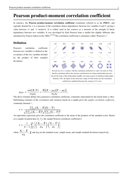
Pearson product-moment correlation coefficient In statistics, the Pearson product-moment correlation coefficient (sometimes referred to as the PMCC , and typically denoted by r ) is a measure of the correlation (linear dependence) between two variables X and Y , giving a value between +1 and −1 inclusive. It is widely used in the sciences as a measure of the strength of linear dependence between two variables. It was developed by Karl Pearson from a similar but slightly different idea introduced by Francis Galton in the 1880s.[1] [2] The correlation coefficient is sometimes called "Pearson's r."Several sets of (x , y ) points, with the correlation coefficient of x and y for each set. Notethat the correlation reflects the noisiness and direction of a linear relationship (top row),but not the slope of that relationship (middle), nor many aspects of nonlinear relationships(bottom). N.B.: the figure in the center has a slope of 0 but in that case the correlationcoefficient is undefined because the variance of Yis zero.DefinitionPearson's correlation coefficientbetween two variables is defined as thecovariance of the two variables dividedby the product of their standarddeviations:The above formula defines the population correlation coefficient, commonly represented by the Greek letter ρ (rho).Substituting estimates of the covariances and variances based on a sample gives the sample correlation coefficient ,commonly denoted r:An equivalent expression gives the correlation coefficient as the mean of the products of the standard scores. Based on a sample of paired data (X i , Y i), the sample Pearson correlation coefficient iswhere , and are the standard score, sample mean, and sample standard deviation respectively.Mathematical propertiesThe absolute value of both the sample and population Pearson correlation coefficients are less than or equal to 1.Correlations equal to 1 or -1 correspond to data points lying exactly on a line (in the case of the sample correlation),or to a bivariate distribution entirely supported on a line (in the case of the population correlation). The Pearson correlation coefficient is symmetric: corr (X ,Y ) = corr (Y ,X ).A key mathematical property of the Pearson correlation coefficient is that it is invariant to separate changes in location and scale in the two variables. That is, we may transform X to a + bX and transform Y to c + dY , where a , b ,c , and d are constants, without changing the correlation coefficient (this fact holds for both the population and sample Pearson correlation coefficients). Note that more general linear transformations do change the correlation:see a later section for an application of this.The Pearson correlation can be expressed in terms of uncentered moments. Since μX = E(X ), σX 2 = E[(X − E(X ))2]= E(X 2) − E 2(X ) and likewise for Y , and sincethe correlation can also be written asAlternative formulae for the sample Pearson correlation coefficient are also available:The above formula conveniently suggests a single-pass algorithm for calculating sample correlations, but, depending on the numbers involved, it can sometimes be numerically unstable.InterpretationThe correlation coefficient ranges from −1 to 1. A value of 1 implies that a linear equation describes the relationship between X and Y perfectly, with all data points lying on a line for which Y increases as X increases. A value of −1implies that all data points lie on a line for which Y decreases as X increases. A value of 0 implies that there is no linear correlation between the variables.More generally, note that (X i − X )(Y i − Y ) is positive if and only if X i and Y i lie on the same side of their respective means. Thus the correlation coefficient is positive if X i and Y i tend to be simultaneously greater than, or simultaneously less than, their respective means. The correlation coefficient is negative if X i and Y i tend to lie on opposite sides of their respective means.Geometric interpretationRegression lines for y=g x (x) [red] and x=g y(y) [blue ]For uncentered data, the correlation coefficientcorresponds with the the cosine of the anglebetween both possible regression lines y=g x (x) andx=g y(y).For centered data (i.e., data which have beenshifted by the sample mean so as to have anaverage of zero), the correlation coefficient canalso be viewed as the cosine of the anglebetween the two vectors of samples drawn fromthe two random variables (see below).Some practitioners prefer an uncentered(non-Pearson-compliant) correlation coefficient.See the example below for a comparison.As an example, suppose five countries are found tohave gross national products of 1, 2, 3, 5, and 8billion dollars, respectively. Suppose these same five countries (in the same order) are found to have 11%, 12%,13%, 15%, and 18% poverty. Then let x and y be ordered 5-element vectors containing the above data: x = (1, 2, 3,5, 8) and y = (0.11, 0.12, 0.13, 0.15, 0.18).By the usual procedure for finding the angle between two vectors (see dot product), the uncentered correlationcoefficient is:Note that the above data were deliberately chosen to be perfectly correlated: y = 0.10 + 0.01 x . The Pearson correlation coefficient must therefore be exactly one. Centering the data (shifting x by E(x ) = 3.8 and y by E(y ) =0.138) yields x = (−2.8, −1.8, −0.8, 1.2, 4.2) and y = (−0.028, −0.018, −0.008, 0.012, 0.042), from whichas expected.Interpretation of the size of a correlation CorrelationNegative Positive None−0.09 to 0.00.0 to 0.09Small−0.3 to −0.10.1 to 0.3Medium−0.5 to −0.30.3 to 0.5Large −1.0 to −0.50.5 to 1.0Several authors [3] have offered guidelines for the interpretation of a correlation coefficient. Cohen (1988),[3] has observed, however, that all such criteria are in some ways arbitrary and should not be observed too strictly. The interpretation of a correlation coefficient depends on the context and purposes. A correlation of 0.9 may be very low if one is verifying a physical law using high-quality instruments, but may be regarded as very high in the social sciences where there may be a greater contribution from complicating factors.InferenceA graph showing the minimum value of Pearson's correlation coefficient that issignificantly different from zero at the 0.05 level, for a given sample size.Statistical inference based on Pearson'scorrelation coefficient often focuses on oneof the following two aims. One aim is to testthe null hypothesis that the true correlationcoefficient is ρ, based on the value of thesample correlation coefficient r . The otheraim is to construct a confidence intervalaround r that has a given probability ofcontaining ρ.Randomization approachesPermutation tests provide a direct approachto performing hypothesis tests andconstructing confidence intervals. Apermutation test for Pearson's correlationcoefficient involves the following two steps:(i) using the original paired data (x i , y i ),randomly redefine the pairs to create a newdata set (x i , y i ′), where the i ′ are a permutation of the set {1,...,n }. The permutation i ′ is selected randomly, with equal probabilities placed on all n ! possible permutations. This is equivalent to drawing the i ′ randomly "without replacement" from the set {1,..., n }. A closely-related and equally-justified (bootstrapping) approach is to separately draw the i and the i ′ "with replacement" from {1,..., n }; (ii) Construct a correlation coefficient r from the randomized data. To perform the permutation test, repeat (i) and (ii) a large number of times. The p-value for the permutation test is one minus the proportion of the r values generated in step (ii) that are larger than the Pearson correlation coefficient that was calculated from the original data. Here "larger" can mean either that the value is larger in magnitude, or larger in signed value, depending on whether a two-sided or one-sided test is desired.The bootstrap can be used to construct confidence intervals for Pearson's correlation coefficient. In the "non-parametric" bootstrap, n pairs (x i , y i ) are resampled "with replacement" from the observed set of n pairs, and the correlation coefficient r is calculated based on the resampled data. This process is repeated a large number of times,and the empirical distribution of the resampled r values are used to approximate the sampling distribution of the statistic. A 95% confidence interval for ρ can be defined as the interval spanning from the 2.5th to the 97.5th percentile of the resampled r values.Approaches based on mathematical approximationsFor approximately Gaussian data, the sampling distribution of Pearson's correlation coefficient approximately follows Student's t-distribution with degrees of freedom N − 2. Specifically, if the underlying variables have abivariate normal distribution, the variablehas a Student's t-distribution in the null case (zero correlation).[4] This also holds approximately even if the observed values are non-normal, provided sample sizes are not very small.[5] For constructing confidence intervals and performing power analyses, the inverse of this transformation is also needed:Alternatively, large sample approaches can be used.Early work on the distribution of the sample correlation coefficient was carried out by R. A. Fisher[6][7] and A. K. Gayen.[8] Another early paper[9] provides graphs and tables for general values of ρ, for small sample sizes, and discusses computational approaches.Fisher TransformationIn practice, confidence intervals and hypothesis tests relating to ρ are usually carried out using the Fisher transformation:If F(r) is the Fisher transformation of r, and n is the sample size, then F(r) approximately follows a normal distribution withand standard errorThus, a z-score isunder the null hypothesis of that , given the assumption that the sample pairs are independent and identically distributed and follow a bivariate normal distribution. Thus an approximate p-value can be obtained from a normal probability table. For example, if z = 2.2 is observed and a two-sided p-value is desired to test the null hypothesis that , the p-value is 2·Φ(−2.2) = 0.028, where Φ is the standard normal cumulative distribution function.Confidence IntervalsTo obtain a confidence interval for ρ, we first compute a confidence interval for F( ):The inverse Fisher transformation bring the interval back to the correlation scale.For example, suppose we observe r = 0.3 with a sample size of n=50, and we wish to obtain a 95% confidence interval for ρ. The transformed value is artanh(r) = 0.30952, so the confidence interval on the transformed scale is 0.30952 ± 1.96/√47, or (0.023624, 0.595415). Converting back to the correlation scale yields (0.024, 0.534).Pearson's correlation and least squares regression analysisThe square of the sample correlation coefficient, which is also known as the coefficient of determination, estimates the fraction of the variance in Y that is explained by X in a linear regression analysis. As a starting point, the total variation in the Yaround their average value can be decomposed as followsiwhere the are the fitted values from the regression analysis. This can be rearranged to giveThe two summands above are the fraction of variance in Y that is explained by X (right) and that is unexplained by X (left).Next, we apply a property of least square regression analysis, that the sample covariance between andis zero. Thus, the sample correlation coefficient between the observed and fitted response values in the regression can be writtenThusis the proportion of variance in Y explained by a linear function of X.Sensitivity to the data distributionExistenceThe population Pearson correlation coefficient is defined in terms of moments, and therefore exists for any bivariate probability distribution for which the population covariance is defined and the marginal population variances are defined and are non-zero. Some probability distributions such as the Cauchy distribution have undefined variance and hence ρ is not defined if X or Y follows such a distribution. In some practical applications, such as those involving data suspected to follow a heavy-tailed distribution, this is an important consideration. However, the existence of the correlation coefficient is usually not a concern; for instance, if the range of the distribution is bounded, ρ is always defined.Large sample propertiesIn the case of the bivariate normal distribution the population Pearson correlation coefficient characterizes the joint distribution as long as the marginal means and variances are known. For most other bivariate distributions this is not true. Nevertheless, the correlation coefficient is highly informative about the degree of linear dependence between two random quantities regardless of whether their joint distribution is normal[1] . The sample correlation coefficient is the maximum likelihood estimate of the population correlation coefficient for bivariate normal data, and is asymptotically unbiased and efficient, which roughly means that it is impossible to construct a more accurate estimate than the sample correlation coefficient if the data are normal and the sample size is moderate or large. For non-normal populations, the sample correlation coefficient remains approximately unbiased, but may not be efficient. The sample correlation coefficient is a consistent estimator of the population correlation coefficient as long as the sample means, variances, and covariance are consistent (which is guaranteed when the law of large numbers can be applied).RobustnessLike many commonly-used statistics, the sample statistic r is not robust[10] , so its value can be misleading if outliers are present[11][12] . Specifically, the PMCC is neither distributionally robust, nor outlier resistant[10] (see Robust statistics#Definition). Inspection of the scatterplot between X and Y will typically reveal a situation where lack of robustness might be an issue, and in such cases it may be advisable to use a robust measure of association. Note however that while most robust estimators of association measure statistical dependence in some way, they are generally not interpretable on the same scale as the Pearson correlation coefficient.Statistical inference for Pearson's correlation coefficient is sensitive to the data distribution. Exact tests, and asymptotic tests based on the Fisher transformation can be applied if the data are approximately normally distributed, but may be misleading otherwise. In some situations, the bootstrap can be applied to construct confidence intervals, and permutation tests can be applied to carry out hypothesis tests. These non-parametric approaches may give more meaningful results in some situations where bivariate normality does not hold. However the standard versions of these approaches rely on exchangeability of the data, meaning that there is no ordering or grouping of the data pairs being analyzed that might affect the behavior of the correlation estimate.A stratified analysis is one way to either accommodate a lack of bivariate normality, or to isolate the correlation resulting from one factor while controlling for another. If W represents cluster membership or another factor that it is desirable to control, we can stratify the data based on the value of W, then calculate a correlation coefficient within each stratum. The stratum-level estimates can then be combined to estimate the overall correlation while controlling for W.[13]Calculating a weighted correlationSuppose observations to be correlated have differing degrees of importance that can be expressed with a weight vector w. To calculate the correlation between vectors x and y with the weight vector w (all of length n),[14][15]•Weighted mean:•Weighted covariance•Weighted correlationRemoving correlationIt is always possible to remove the correlation between random variables with a linear transformation, even if the relationship between the variables is nonlinear. A presentation of this result for population distributions is given by Cox & Hinkley.[16]A corresponding result exists for sample correlations, in which the sample correlation is reduced to zero. Suppose a vector of n random variables is sampled m times. Let X be a matrix where is the j th variable of sample i. Letbe an m by m square matrix with every element 1. Then D is the data transformed so every random variable has zero mean, and T is the data transformed so all variables have zero mean and zero correlation with all other variables - the moment matrix of T will be the identity matrix. This has to be further divided by the standard deviation to get unit variance. The transformed variables will be uncorrelated, even though they may not be independent.where an exponent of -1/2 represents the matrix square root of the inverse of a matrix. The covariance matrix of T will be the identity matrix. If a new data sample x is a row vector of n elements, then the same transform can be applied to x to get the transformed vectors d and t:This decorrelation is related to Principal Components Analysis for multivariate data.Reflective correlationThe reflective correlation is a variant of Pearson's correlation in which the data are not centered around their mean values. The population reflective correlation isThe reflective correlation is symmetric, but it is not invariant under translation:The sample reflective correlation isThe weighted version of the sample reflective correlation isReferences[1]J. L. Rodgers and W. A. Nicewander. Thirteen ways to look at the correlation coefficient (/stable/2685263). TheAmerican Statistician, 42(1):59–66, February 1988.[2]Stigler, Stephen M. (1989). "Francis Galton's Account of the Invention of Correlation" (/stable/2245329). StatisticalScience4 (2): 73–79. doi:10.1214/ss/1177012580. .[3]Cohen, J. (1988). Statistical power analysis for the behavioral sciences (2nd ed.)[4]N.A Rahman, A Course in Theoretical Statistics; Charles Griffin and Company, 1968[5]Kendall, M.G., Stuart, A. (1973)The Advanced Theory of Statistics, Volume 2: Inference and Relationship, Griffin. ISBN 0852642156(Section 31.19)[6]Fisher, R.A. (1915). "Frequency distribution of the values of the correlation coefficient in samples from an indefinitely large population".Biometrika10 (4): 507–521. doi:10.1093/biomet/10.4.507.[7]Fisher, R.A. (1921). "On the probable error of a coefficient of correlation deduced from a small sample" (/2440/15169) (PDF). Metron1 (4): 3–32. . Retrieved 2009-03-25.[8]Gayen, A.K. (1951). "The frequency distribution of the product moment correlation coefficient in random samples of any size draw fromnon-normal universes". Biometrika38: 219–247. doi:10.1093/biomet/38.1-2.219.[9]Soper, H.E., Young, A.W., Cave, B.M., Lee, A., Pearson, K. (1917). "On the distribution of the correlation coefficient in small samples.Appendix II to the papers of "Student" and R. A. Fisher. A co-operative study", Biometrika, 11, 328-413. doi:10.1093/biomet/11.4.328[10]Wilcox, Rand R. (2005). Introduction to robust estimation and hypothesis testing. Academic Press.[11]Devlin, Susan J; Gnanadesikan, R; Kettenring J.R. (1975). "Robust Estimation and Outlier Detection with Correlation Coefficients" (http:///stable/2335508). Biometrika62 (3): 531–545. doi:10.1093/biomet/62.3.531. .[12]Huber, Peter. J. (2004). Robust Statistics. Wiley.[13]Multivariable Analysis- A Practical Guide for Clinicians. 2nd Edition. (/uk/catalogue/catalogue.asp?isbn=052154985X&ss=exc) Mitchell H. Katz. University of California, San Francisco. ISBN 9780521549851. ISBN 052154985X DOI:10.2277/052154985X[14]/Archive/sci.stat.math/2006-02/msg00171.html[15] A MATLAB Toolbox for computing Weighted Correlation Coefficients (/matlabcentral/fileexchange/20846)[16]Cox, D.R., Hinkley, D.V. (1974) Theoretical Statistics, Chapman & Hall (Appendix 3) ISBN 0412124203Article Sources and Contributors10 Article Sources and ContributorsPearson product-moment correlation coefficient Source: /w/index.php?oldid=406110938 Contributors: AgarwalSumeet, Albmont, Amillar, Arbitrary username,Arcadian, AxelBoldt, Baccyak4H, Beno1000, Bobo192, Bramschoenmakers, Can't sleep, clown will eat me, Chris53516, Cometstyles, Countchoc, Damian Yerrick, Deditos, Delirium, Denfjättrade ankan, DerHexer, Dfarrar, Discospinster, Dpryan, Dr.enh, Drbreznjev, Dysprosia, FrancisTyers, G-J, G716, Garion96, Giftlite, Gringotumadre, Ichbin-dcw, Ignoramibus,Irregulargalaxies, JamesBWatson, JeremyA, Jfitzg, Jmath666, JohnEBredehoft, JorisvS, Jtneill, Juancitomiguelito, Karada, Karl Dickman, Karol Langner, Kinneyboy90, Kku, Kyawtun,Landroni, Ldm, MER-C, Mahahahaneapneap, Male1979, Mc4932, Mcld, Melcombe, Michael Hardy, Mild Bill Hiccup, Mmmready, MrOllie, MrYdobon, NeonMerlin, Notheruser, O18, Parodi, Pearle, Qniemiec, Qwfp, Rajah, Ramkgupta1, RedCoat10, Rgclegg, Rich Farmbrough, Rifleman 82, Rjwilmsi, Skbkekas, Stewartadcock, Sykko, Talgalili, Tdslk, Tellyaddict, Tesi1700, Tomharrison, Trontonian, Versus22, Vinhtantran, Vrenator, WikHead, Wikifriend pt001, Wootini, Xenoglossophobe, Yamiken, Yerpo, 170 anonymous editsImage Sources, Licenses and ContributorsImage:Correlation examples.png Source: /w/index.php?title=File:Correlation_examples.png License: Public Domain Contributors: Original uploader was Imagecreator at en.wikipediaFile:Regression lines.png Source: /w/index.php?title=File:Regression_lines.png License: Creative Commons Attribution-Sharealike 3.0 Contributors: User:Qniemiec Image:correlation significance.svg Source: /w/index.php?title=File:Correlation_significance.svg License: Creative Commons Attribution 3.0 Contributors:User:SkbkekasLicenseCreative Commons Attribution-Share Alike 3.0 Unported/licenses/by-sa/3.0/。
hodges-lehmann位置偏移估计值

在统计学中,Hodges-Lehmann位置偏移估计值是一种用于衡量两组数据差异的非参数方法。
它的计算方法是取每个组合的差值,然后对这些差值取中位数。
这个估计值不仅不受异常值的影响,而且对数据分布的偏斜和尺度也不敏感,因此在一定程度上具有较好的鲁棒性。
我们可以从简单的例子开始,来理解Hodges-Lehmann位置偏移估计值的计算过程。
假设我们有两组数据,分别是A组和B组。
我们要计算这两组数据的位置偏移估计值。
1. 我们需要对所有A组和B组中的数据进行配对组合,计算出所有配对的差值。
2. 将这些差值进行排序,找出其中位数的差值,即为Hodges-Lehmann位置偏移估计值。
举个简单的例子,假设A组数据为[3, 4, 5, 6, 7],B组数据为[2, 4, 5, 7, 8]。
我们可以计算出所有配对的差值为[-1, 0, 0, 1, 1, 0, 1, 2, 3],然后找出其中位数的差值,即为0。
以上就是Hodges-Lehmann位置偏移估计值的简单计算过程。
接下来,我们可以探讨一些在实际应用中的相关问题。
Hodges-Lehmann位置偏移估计值适用于什么样的数据类型?Hodges-Lehmann位置偏移估计值适用于连续变量的数据,因为它是基于差值的中位数计算的,而对于类别型数据这种计算方法就不适用了。
Hodges-Lehmann位置偏移估计值在哪些领域有着广泛的应用?Hodges-Lehmann位置偏移估计值通常用于比较两组数据的位置差异,例如在医学研究中比较两种治疗方法的效果、在市场营销中比较不同产品的销售情况等。
我们还可以思考Hodges-Lehmann位置偏移估计值的局限性是什么?尽管Hodges-Lehmann位置偏移估计值对异常值具有较好的鲁棒性,但是它对样本量的要求较高,当样本量较小时,其稳定性和准确性就会受到影响。
Hodges-Lehmann位置偏移估计值是一种非参数方法,它通过计算单个配对的差值的中位数来衡量两组数据的位置差异,具有鲁棒性和不受异常值影响的优点。
correlation 标准流程
correlation 标准流程英文回答:Correlation.Correlation is a statistical measure that expresses the extent to which two variables are linearly related. It is a value between -1 and 1, where -1 indicates a perfect negative correlation, 0 indicates no correlation, and 1 indicates a perfect positive correlation.The correlation coefficient is calculated by dividing the covariance of the two variables by the product of their standard deviations. The covariance is a measure of how much the two variables vary together, and the standard deviation is a measure of how much each variable varies on its own.Correlation is a useful tool for understanding the relationship between two variables. It can be used toidentify trends, make predictions, and test hypotheses. However, it is important to note that correlation does not imply causation. Just because two variables are correlated does not mean that one causes the other.Types of Correlation.There are three main types of correlation:Positive correlation: This type of correlation occurs when two variables increase or decrease together. For example, the number of hours you study for a test and your score on the test are positively correlated.Negative correlation: This type of correlation occurs when one variable increases and the other variable decreases. For example, the amount of money you spend ongas and your car's gas mileage are negatively correlated.No correlation: This type of correlation occurs when there is no relationship between two variables. For example, the number of times you flip a coin and the number of headsyou get are not correlated.Strength of Correlation.The strength of a correlation is determined by the absolute value of the correlation coefficient. The closer the correlation coefficient is to 1 or -1, the stronger the correlation. A correlation coefficient of 0 indicates that there is no correlation between the two variables.Significance of Correlation.The significance of a correlation is determined by the p-value. The p-value is the probability of obtaining a correlation coefficient as large as or larger than the one that was observed, assuming that there is no correlation between the two variables. A p-value less than 0.05 is considered to be statistically significant.Correlation Analysis.Correlation analysis is a statistical technique that isused to identify and measure the relationship between two or more variables. Correlation analysis can be used to:Identify trends.Make predictions.Test hypotheses.Control for confounding variables.Correlation analysis is a valuable tool for understanding the relationships between variables. However, it is important to note that correlation does not imply causation.中文回答:相关性。
相关分析(Correlate)
相关分析(Correlate)Correlation and dependenceIn statistics, correlation and dependence are any of a broad class of statistical relationships between two or more random variables or observed data values.Correlation is computed(用...计算)into what is known as the correlation coefficient(相关系数), which ranges between -1 and +1. Perfect positive correlation (a correlation co-efficient of +1) implies(意味着)that as one security(证券)moves, either up or down, the other security will move in lockstep(步伐一致的), in the same direction. Alternatively(同样的), perfect negative correlation means that if one security moves in either direction the security that is perfectly negatively correlated will move by an equal amount in the opposite(相反的)direction. If the correlation is 0, the movements of the securities are said to have no correlation; they are completely random(随意、胡乱).There are several correlation coefficients, often denoted(表示、指示)ρ or r, measuring(衡量、测量)the degree of correlation. The most common of these is the Pearson correlation coefficient, which is sensitive only to a linear(只进行两变量线性分析)relationship between two variables (which may exist even if one is a nonlinear function of the other).Other correlation coefficients have been developed to be more robust(有效的、稳健)than the Pearson correlation, or more sensitive to nonlinear relationships.Rank(等级)correlation coefficients, such as Spearman's rank correlation coefficient and Kendall's rank correlation coefficient (τ) measure the extent(范围)to which, as one variable increases, the other variable tends to increase, without requiring(需要、命令)that increase to be represented by a linear relationship. If, as the one variable(变量)increases(增加), the other decreases, the rank correlation coefficients will be negative. It is common to regard these rank correlation coefficients as alternatives to Pearson's coefficient, used either to reduce the amount of calculation or to make the coefficient less sensitive to non-normality in distributions(分布). However, this view has little mathematical basis, as rank correlation coefficients measure a different type of relationship than the Pearson product-moment correlation coefficient, and are best seen as measures of a different type of association, rather than as alternative measure of the population correlation coefficient.Common misconceptions(错误的想法)Correlation and causality(因果关系)The conventional(大会)dictum(声明)that "correlation does not imply causation" means that correlation cannot be used to infer a causal relationship between the variables.Correlation and linearityFour sets of data with the same correlation of 0.816The Pearson correlation coefficient indicates the strength of a linear relationship between two variables, but its value generally does not completely characterize their relationship. In particular, if the conditional mean of Y given X, denoted E(Y|X), is not linear in X, the correlation coefficient will not fully determine the form ofE(Y|X).The image on the right shows scatterplots(散点图)of Anscombe's quartet, a set of four different pairs of variables created by Francis Anscombe. The four y variables have the same mean (7.5), standard deviation (4.12), correlation (0.816) and regression line (y = 3 + 0.5x). However, as can be seen on the plots, the distribution of the variables is very different. The first one (top left) seems to be distributed normally, and corresponds to what one would expect when considering two variables correlated and following the assumption of normality. The second one (top right) is not distributed normally; while an obvious relationship between the two variables can be observed, it is not linear. In this case the Pearson correlation coefficient does not indicate that there is an exact functional relationship: only the extent to which that relationship can be approximated(大概)by a linear relationship. In the third case (bottom left), the linear relationship is perfect, except for one outlier which exerts enough influence to lower the correlation coefficient from 1 to0.816. Finally, the fourth example (bottom right) shows another example when one outlier(异常值)is enough to produce a high correlation coefficient, even though the relationship between the two variables is not linear.(离群值可降低、也可以增加数据的相关性。
pearson相关系数表
pearson相关系数表 Pearson相关系数表
引言: Pearson相关系数是一种衡量两个变量之间线性关系强度的统计指标。它可以帮助我们了解两个变量之间的相关程度以及它们的变化趋势。本文将介绍Pearson相关系数的定义、计算方法和应用场景,并提供一个Pearson相关系数表供读者参考。
一、Pearson相关系数的定义: Pearson相关系数是用来衡量两个变量之间线性关系的强度和方向的统计指标。它的取值范围为-1到1之间,其中-1表示完全负相关,1表示完全正相关,0表示无相关。Pearson相关系数是通过计算两个变量之间的协方差来得出的。
二、Pearson相关系数的计算方法: 计算Pearson相关系数需要先计算两个变量的协方差和它们的标准差。协方差表示两个变量的变化趋势是否一致,标准差表示变量的离散程度。Pearson相关系数的计算公式如下:
r = Cov(X,Y) / (σ(X) * σ(Y)) 其中,r表示Pearson相关系数,Cov(X,Y)表示X和Y的协方差,σ(X)和σ(Y)表示X和Y的标准差。 三、Pearson相关系数的应用场景: 1. 金融领域:Pearson相关系数可以用来衡量两个股票价格变动之间的相关性。通过分析相关系数,投资者可以了解不同股票之间的关联程度,从而制定更有效的投资策略。 2. 社会科学研究:Pearson相关系数可以用来分析不同变量之间的关系,如收入和教育水平之间的相关性、犯罪率和失业率之间的相关性等。这些分析结果可以帮助研究者深入理解社会现象,并提供政策建议。 3. 市场调研:Pearson相关系数可以用来分析不同产品之间的关联程度,从而帮助企业制定市场策略。例如,一个公司可以通过分析相关系数来确定不同产品之间的替代关系,以便在市场竞争中做出相应调整。
四、Pearson相关系数表: 以下是一个Pearson相关系数表,展示了不同相关系数值对应的相关程度:
计量经济学术语
计量经济学术语A校正R2(Adjusted R-Squared):多元回归分析中拟合优度的量度,在估计误差的方差时对添加的解释变量用一个自由度来调整。
对立假设(Alternative Hypothesis):检验虚拟假设时的相对假设。
AR(1)序列相关(AR(1) Serial Correlation):时间序列回归模型中的误差遵循AR(1)模型。
渐近置信区间(Asymptotic Confidence Interval):大样本容量下近似成立的置信区间。
渐近正态性(Asymptotic Normality):适当正态化后样本分布收敛到标准正态分布的估计量。
渐近性质(Asymptotic Properties):当样本容量无限增长时适用的估计量和检验统计量性质。
渐近标准误(Asymptotic Standard Error):大样本下生效的标准误。
渐近t 统计量(Asymptotic t Statistic):大样本下近似服从标准正态分布的t统计量。
渐近方差(Asymptotic Variance):为了获得渐近标准正态分布,我们必须用以除估计量的平方值。
渐近有效(Asymptotically Efficient):对于服从渐近正态分布的一致性估计量,有最小渐近方差的估计量。
渐近不相关(Asymptotically Uncorrelated):时间序列过程中,随着两个时点上的随机变量的时间间隔增加,它们之间的相关趋于零。
衰减偏误(Attenuation Bias):总是朝向零的估计量偏误,因而有衰减偏误的估计量的期望值小于参数的绝对值。
自回归条件异方差性(Autoregressive Conditional Heteroskedasticity, ARCH):动态异方差性模型,即给定过去信息,误差项的方差线性依赖于过去的误差的平方。
一阶自回归过程[AR(1)](Autoregressive Process of Order One [AR(1)]):一个时间序列模型,其当前值线性依赖于最近的值加上一个无法预测的扰动。