A Switching Control Scheme for Underactuated CartPole Systems with Aggressive Swingup

合集下载

Adaptive Trajectory Tracking Control of Skid-Steered Mobile Robots

1-4244-0602-1/07/$20.00 ©2007 IEEE.
2605
Authorized licensed use limited to: NANKAI UNIVERSITY. Downloaded on March 2, 2009 at 02:33 from IEEE Xplore. Restrictions apply.
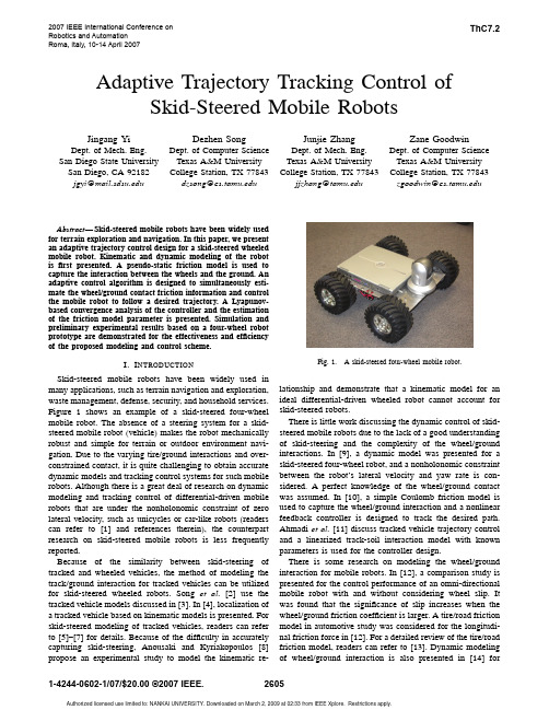
I. I NTRODUCTION Skid-steered mobile robots have been widely used in many applications, such as terrain navigation and exploration, waste management, defense, security, and household services. Figure 1 shows an example of a skid-steered four-wheel mobile robot. The absence of a steering system for a skidsteered mobile robot (vehicle) makes the robot mechanically robust and simple for terrain or outdoor environment navigation. Due to the varying tire/ground interactions and overconstrained contact, it is quite challenging to obtain accurate dynamic models and tracking control systems for such mobile robots. Although there is a great deal of research on dynamic modeling and tracking control of differential-driven mobile robots that are under the nonholonomic constraint of zero lateral velocity, such as unicycles or car-like robots (readers can refer to [1] and references therein), the counterpart research on skid-steered mobile robots is less frequently reported. Because of the similarity between skid-steering of tracked and wheeled vehicles, the method of modeling the track/ground interaction for tracked vehicles can be utilized for skid-steered wheeled robots. Song et al. [2] use the tracked vehicle models discussed in [3]. In [4], localization of a tracked vehicle based on kinematic models is presented. For skid-steered modeling of tracked vehicles, readers can refer to [5]–[7] for details. Because of the difﬁculty in accurately capturing skid-steering, Anousaki and Kyriakopoulos [8] propose an experimental study to model the kinematic re-

Computers & Electrical Engineering样文

Adaptive control of dynamic mobile robots withnonholonomic constraintsFarzad Pourboghrat *,Mattias P.KarlssonDepartment of Electrical and Computer Engineering,Southern Illinois University,Carbondale,IL 62901-6603,USAReceived 16November 1999;accepted 22August 2000AbstractThis paper presents adaptive control rules,at the dynamics level,for the nonholonomic mobile robots with unknown dynamic parameters.Adaptive controls are derived for mobile robots,using backstepping technique,for tracking of a reference trajectory and stabilization to a ﬁxed posture.For the tracking problem,the controller guarantees the asymptotic convergence of the tracking error to zero.For stabili-zation,the problem is converted to an equivalent tracking problem,using a time varying error feedback,before the tracking control is applied.The designed controller ensures the asymptotic zeroing of the sta-bilization error.The proposed control laws include a velocity/acceleration limiter that prevents the robot Õs wheels from slipping.Ó2002Elsevier Science Ltd.All rights reserved.Keywords:Mobile robot;Nonholonomic constraint;Dynamics level motion control;Stabilization and tracking;Adaptive control;Backstepping technique;Asymptotic stability1.IntroductionMotion control of mobile robots has found considerable attention over the past few years.Most of these reports have focused on the steering or trajectory generation problem at the ki-nematics level i.e.,considering the system velocities as control inputs and ignoring the mechanical system dynamics [1–3].Very few reports have been published on control design in the presence of uncertainties in the dynamic model [4].Some preliminary results on control of nonholonomic systems with uncertainties are given in Refs.[4–6].Two of the most important control problems concerning mobile robots are tracking of a refer-ence trajectory and stabilization to a ﬁxed posture.The tracking problem has received solutions *Corresponding author.Tel.:+1-618-453-7026.E-mail address:pour@ (F.Pourboghrat).0045-7906/02/$-see front matter Ó2002Elsevier Science Ltd.All rights reserved.PII:S0045-7906(00)00053-7242 F.Pourboghrat,M.P.Karlsson/Computers and Electrical Engineering28(2002)241–253including classical nonlinear control techniques[1,2,7].The basic idea is to have a reference car that generates a trajectory for the mobile robot to follow.In Refs.[1,2],nonlinear velocity control inputs were deﬁned that made the tracking error go to zero as long as the reference car was moving.In Ref.[7],they used input–output linearization to make a mobile platform follow a desired trajec-tory.The problem of stabilization about aﬁxed posture has been shown to be rather complicated. This is due to violating the BrockettÕs condition[8],which states that for nonholonomic systems a single equilibrium solution cannot be asymptotically stabilized using continuous static state feedback[9,10].The BrockettÕs condition essentially states that for nonholonomic systems an equilibrium solution can be asymptotically stabilized only by either a time varying,a discontin-uous,or a dynamic state feedback.In addressing the above problem,in Ref.[10]a smooth feedback control was presented for the kinematics control problem resulting in a globally marginally stable closed loop system.They also designed a smooth feedback control for a dynamical state-space model resulting in a Lagrange stable closed loop system,as deﬁned in their paper.A two dimensional Lyapunov function was utilized in Ref.[3]to prescribe a set of desired trajectories to navigate a mobile robot to a speciﬁed conﬁguration.The desired trajectory was then tracked using sliding mode control,resulting in discontinuous control signals.The mobile robot was shown to be exponentially stable for a class of quadratic Lyapunov functions.In Ref.[9],they formulated a reduced order state equation for a class of nonholonomic systems.Several other researchers have later used this reduced order state equation in their studies.In Ref.[4],the problem of controlling nonholonomic mechanical sys-tems with uncertainties,at the dynamics level,was ing the reduced state equation in Ref.[9],they proposed an adaptive controller for a number of important nonholonomic control problems,including stabilization of general systems to an equilibrium manifold and stabilization of diﬀerentiallyﬂat and Caplygin systems to an equilibrium point.In Ref.[2],they gave several examples on how the stabilization problem can be solved for a mobile robot at the kinematics level.Their solutions included time-varying control,piecewise continuous control,and time-varying piecewise continuous control.They also showed how a solution to the tracking problem could be extended to work even for the stabilization problem.Here,we present adaptive control schemes for the tracking problem and for the problem of stabilization to aﬁxed posture when the dynamic model of the mobile robot contains unknown parameters.Our work is based on,and can be seen as an extension of,the work presented in Refs. [1,2].Using backstepping technique we derive adaptive control laws that work even when the model of the dynamical system contains uncertainties in the form of unknown constants.The assumption for the uncertainty in robotÕs parameters,particularly the mass,and hence the inertia, can be justiﬁed in real applications such as in automotive manufacturing industry and warehouses, where the robots are to move a variety of parts with diﬀerent shapes and masses.In these cases,the robotÕs mass and inertia may vary up to10%or20%,justifying an adaptive control approach.2.Dynamic model of mobile robotHere,we consider a three-wheeled mobile robot moving on a horizontal plane(Fig.1).The mobile robot features two diﬀerentially driven rear wheels and a castor front wheel.The radius ofthe wheels is denoted r and the length of the rear wheel axis is 2l .Inputs to the system are two torques T 1and T 2,provided by two motors attached to the rear wheels.The dynamic model for the above wheeled-mobile robot is given by Refs.[10,11].€x ¼k m sin /þb 1u 1cos /€y ¼Àk cos /þb 1u 1sin /€/¼b 2u 28><>:ð1Þ_x sin /À_y cos /¼0ð2Þwhere b 1¼1=ðrm Þ,b 2¼l =ðrI Þ,and that m and I denote the mass and the moment of inertia of the mobile robot,respectively.Also,u 1¼T 1þT 2and u 2¼T 1ÀT 2are the control inputs,and k is the Lagrange multiplier,given by k ¼Àm _/_x cos /þ_y sin /ðÞ.Here,it is assumed that b 1and b 2are unknown constants with known signs.The assumption that the signs of b 1and b 2are known is practical since b 1and b 2represent combinations of the robot Õs mass,moment of inertia,wheel radius,and distance between the rear wheels.Eq.(2)is the nonholonomic constraint,coming from the assumption that the wheels do not slip.The triplet vector function q t ðÞ¼x t ðÞ;y t ðÞ;/t ðÞ½ T denotes the trajectory (position and orientation)of the robot with respect to a ﬁxed workspace frame.That is,at any given time,q ¼½x ;y ;/ T describes the robot Õs conﬁguration (posture)at that time.We assume that,at any time,the robot Õs posture,q ¼½x ;y ;/ T ,as well as its derivative,_q¼½_x ;_y ;_/ T ,are available for feedback.3.Tracking problem deﬁnitionThe tracking problem consists of making the trajectory q of the mobile robot follow a reference trajectory q r .The reference trajectory q r t ðÞ¼x r t ðÞ;y r t ðÞ;/r t ðÞ½ T is generated by a reference ve-hicle/robot whose equations are_xr ¼v r cos /r _y r¼v r sin /_/r ¼x r8<:ð3ÞThe subscript ‘‘r’’stands for reference,and v r and x r are the reference translational (linear)velocity and the reference rotational (angular)velocity,respectively.We assume that v r and x r ,as well as their derivatives are available and that they all are bounded.Assumption A 1.For the tracking problem it is assumed that the reference velocities v r and x r do not both go to zero simultaneously.That is,it is assumed that at any time either lim t !1v r t ðÞ90and/or lim t !1x r t ðÞ90.The tracking problem,under the Assumption A 1,is to ﬁnd a feedback control law u 1u 2 ¼u q ;_q ;q r ;v r ;x r ;_v r ;_x r ðÞsuch that lim t !1~q t ðÞ¼0,where ~q t ðÞ¼q r t ðÞÀq t ðÞis deﬁned as the trajectory tracking error.As in Ref.[1],we deﬁne the equivalent trajectory tracking error ase ¼T ~qð4Þwhere e ¼½e 1;e 2;e 3 T ,and T ¼cos /sin /0Àsin /cos /00010@1A .Note that since T matrix is nonsingular,e is nonzero as long as ~q¼0.Assuming that the angles /r and /are given in the range ½Àp ;p ,we have the equivalent trajectory tracking error e ¼0only if q ¼q r .The purpose of the tracking controller is to force the equivalent trajectory tracking error e to 0.In the sequel we refer to e as the trajectory tracking error.Using the nonholonomic constraint (2),the derivative of the trajectory tracking error given in Eq.(4)can be written as,[1],_e1¼e 2x Àv þv r cos e 3_e 2¼Àe 1x þv r sin e 3_e3¼x r Àx 8<:ð5Þwhere v and x are the translational and rotational velocities of the mobile robot,respectively,and are expressed asv ¼_xcos /þ_y sin /x ¼_/ð6Þ4.Tracking controller designHere,the goal is to design a controller to force the tracking error e ¼½e 1;e 2;e 3 T to ing backstepping technique,since the actual control variables u 1and u 2do not appear in Eq.(5),we consider variables v and x as virtual controls.Let v d and x d denote the desired virtual controls for the mobile robot.That is,with v d and x d the trajectory tracking error e converges tozero asymptotically.Also let us deﬁne ~vand ~x as virtual control errors.Then,v and x can be written asv ¼v d þ~vx ¼x d þ~x ð7Þ244 F.Pourboghrat,M.P.Karlsson /Computers and Electrical Engineering 28(2002)241–253Let us choose the virtual controls v d and x d ,asv d v r ;x r ;e 1;e 3ðÞ¼v r cos e 3þk 1v r ;x r ðÞe 1x d v r ;x r ;e 2;e 3ðÞ¼x r þk 2v r e 2þk 3v r ;x r ðÞsin e 3ð8Þwhere k 2is a positive constant and k 1ðÁÞand k 3ðÁÞare bounded continuous functions with bounded ﬁrst derivatives,strictly positive on R ÂR -ð0;0Þ.Observe that our approach from here on is general for any v d and x d (with well deﬁned ﬁrst derivatives),i.e.any diﬀerentiable control law that makes the kinematics model of the mobile robot track a desired trajectory can be used instead of Eq.(8).Eq.(8)is similar to the control law proposed by Ref.[1],but with the advantage,as we are going to prove later,that it can be used to track any reference trajectory as long as As-sumption A 1holds.Now,consider the following adaptive control scheme:u 1¼^b 1ðÀc 1~v þe 1þ_v d Þu 2¼^b 2 Àc 2~x þ1k 2sin e 3þ_x d _^b 1¼Àc 1sign b 1ðÞ~v ðÀc 1~v þe 1þ_v d Þ_^b 2¼Àc 2sign b 2ðÞ~x Àc 2~x þ1k 2sin e 3þ_x d ð9Þwhere c 1,c 2,c 1,and c 2are positive constants and ^b 1is an estimate of b 1¼1=b 1and ^b 2is an estimate of b 2¼1=b 2.Result 1.If Assumption A 1holds ,then the adaptive control scheme (9)makes the origin e ¼0uniformly asymptotically stable.Proof .Consider the following Lyapunov function candidateV 1¼12e 21Àþe 22Áþ1k 21ðÀcos e 3Þð10Þwhere k 2is a positive constant.Clearly V 1is positive deﬁnite and V 1¼0only if e ¼0.Taking the time derivative of V 1,we obtain_V 1¼e 1ðÀv þv r cos e 3Þþe 2v r sin e 3þ1k 2sin e 3x r ðÀx Þð11ÞFurthermore,using Eqs.(7)and (8),we have_V 1¼Àk 1e 21Àk 3k 2sin 2e 3À~v e 1À~x 1k 2sin e 3ð12ÞIn view of Eqs.(1),(2)and (6),we ﬁnd the time derivatives of ~vand ~x ,as _~v¼_v À_v d ¼€x cos /À_x sin /_/þ€y sin /þ_y cos /_/À_v d ¼b 1u 1À_v d _~x ¼_x À_x d ¼€/À_x d ¼b 2u 2À_x d ð13ÞF.Pourboghrat,M.P.Karlsson /Computers and Electrical Engineering 28(2002)241–253245Consider the Lyapunov function candidateV2¼V1þ12ð~v2þ~x2Þþb1j j2c1~b21þb2j j2c2~b22ð14Þwhere~b1¼b1À^b1¼1=b1À^b1and~b2¼b2À^b2¼1=b2À^b2.Considering Eq.(9)we get:_V 2¼Àk1e21Àk3k2sin2e3Àc1~v2Àc2~x260ð15ÞSince V2is bounded from below and_V2is negative semi-deﬁnite,V2converges to aﬁnite limit. Also,V2,as well as,e1,e2,e3,~v,~x,^b1,and^b2are all bounded.Furthermore,using Eqs.(5),(7)–(9)and(13),the second derivative of V2can be written as€V 2¼À2k1e1e2ðx rþk2v r e2þk3sin e3þ~xÞþ2k1e1ðk1e1þ~vÞÀ_k1e21þ2k3k2cos e3sin e3ðk2v r e2þk3sin e3þ~xÞÀ_k3k2sin2e3À2c1~vðb1^b1ðÀc1~vþe1þ_v dÞÀ_v dÞÀ2c2~x b2^b2Àc2~xþ1k2sin e3þ_x dÀ_x dð16Þwhich from the properties of k1,k2,and k3,the assumption that v r and x r and their derivatives are bounded,and from the above results,can be shown to be bounded,i.e.,_V2is uniformly contin-uous.Since V2ðtÞis diﬀerentiable and converges to some constant value and that€V2is bounded,by BarbalatÕs lemma,_V2tðÞ!0as t!1.This in turn implies that e1,e3,~v,and~x converge to zero [12,13].To show that e2also goes to zero,note that,using the above results,theﬁrst error equation can be written as_e1¼e2x rÀk1e1ð17ÞThe second derivative of e1is€e1¼_x r e2þx rðÀe1xþv r sin e3ÞÀk1e2x rðÀk1e1ÞÀ_k1e1ð18Þwhich can be shown to be bounded by once again using the properties of k1,the assumptions on v r and x r,and Eqs.(7)and(8).Since e1is diﬀerentiable and converges to zero and€e1is bounded,by BarbalatÕs lemma,_e1,and hence,e2x r tend to zero.Proceeding in the same manner,the third error equation can be written as_e3¼Àk2v r e2Àk3sin e3ð19Þand its second derivative can be shown to be bounded.Since e3is diﬀerentiable and converges to zero and€e3is bounded,again by BarbalatÕs lemma,_e3!0as t!1.Hence,k2v r e2and thus v r e2 tend to zero as t!1.Clearly,both v r e2and x r e2converge to zero.However,since v r and x r do not both tend to zero(by Assumption A1),e2must converge to zero.That is,e1,e2,e3,~v,and~x must all converge to zero.hIn Section3,we demonstrated that the system is stable if k2is a positive constant,and that k1ðÁÞand k3ðÁÞare bounded continuous functions with boundedﬁrst derivatives and are strictly positive on RÂR-ð0;0Þ.To get a better understanding on how the control gains aﬀect the response of the system,we write the equations for the closed loop system when~v and~x are equal to zero as[1] 246 F.Pourboghrat,M.P.Karlsson/Computers and Electrical Engineering28(2002)241–253_e¼Àk 1e 1þx r þk 2v r e 2þk 3sin e 3ðÞe 2Àx r þk 2v r e 2þk 3sin e 3ðÞe 1þv r sin e 3Àk 2v r e 2Àk 3sin e 30@1A ð20ÞBy linearizing the diﬀerential equation (20)around e ¼0,we get_e¼Ae ð21Þwhere A ¼Àk 1x r 0Àx r 0v r 0Àk 2v r Àk 30@1A ð22ÞTo simplify the analysis,we assume that v r and x r are constants.The system Õs closed loop poles are now equal to the roots of the following characteristic polynomial equation:s ðþ2nx 0Þs 2Àþ2nx 0s þx 20Áð23Þwhere n and x 0are positive real numbers.The corresponding control gains arek 1¼2nx 0k 2¼x 20Àx 2r v 2r k 3¼2nx 0ð24ÞWith a ﬁxed pole placement strategy (n and x 0are constant),the control gain k 2increaseswithout bound when v r tends to zero.One way to avoid this is by letting the closed loop polesdepend on the values of v r and x r .As in Ref.[2],we choose x 0¼x 2r þbv 2r ÀÁð1=2Þwith b >0.The control gains then becomek 1¼2n x 2r Àþbv 2rÁ1=2k 2¼b k 3¼2n x 2r Àþbv 2r Á1=2ð25Þand the resulting control is now deﬁned for any values of v r and x r .In the above,it is shown that the proposed algorithm works for any desired velocities,ðv d ;x d Þ.However,in practice,if the tracking errors initially are large or if the reference trajectory does not have a continuous curvature (e.g.,if the reference trajectory is a straight line connected to a circle segment),either or both of the virtual reference velocities in Eq.(8)might become too large for a real robot to attain in practice.Hence,the translational/rotational acceleration might become too large causing the robot to slip [1].In order to prevent the mobile robot from slipping,in a real application,a simple velocity/acceleration limiter may be implemented [1],as shown in Fig.2.This limits the virtual reference velocities ðv d ;x d Þby constants ðv max ;x max Þand the virtual referenceaccelerations ða ;a Þby constants ða max ;a max Þ,where a ¼_vd and a ¼_x d are the virtual reference accelerations.In practice,these parameters must be determined experimentally as the largest values with which the mobile robot never slips.F.Pourboghrat,M.P.Karlsson /Computers and Electrical Engineering 28(2002)241–253247An important advantage of adding the limiter is that it lowers the control gains indirectly only when the tracking errors are large,i.e.,when too high a gain could cause the robot to slip,while for small tracking errors it does not aﬀect the performance at all.Thus,by using the limiter one can have higher control gains for small tracking errors to allow for better tracking,while letting the limiter to‘‘scale down’’the gains,indirectly,for large tracking errors,to prevent the robot from slipping.5.Simulation results for tracking control problemHere,the results of computer simulation,using MATLAB/SIMULINK,are presented for a mobile robot with the proposed tracking control and with the velocity/acceleration limiter.The computer simulations for the above controller without the limiter,although not shown here,produce similar results,but with somewhat diﬀerent transient characteristics.All simulations have the common parameters of c1¼c2¼100,c1¼c2¼10and b¼250.Also selected are,the damping factor n¼1,v max¼1:5m/s,x max¼3rad/s,a max¼5m/s2and a max¼25rad/s2.Moreover,the robotÕs dy-namic parameters are chosen as b1¼b2¼0:5,which are assumed to be unknown to the con-troller,but with known signs.Simulation results for the case where the reference trajectory is a straight line are shown in Figs. 3and4for t2½0;10 .The reference trajectory is given by x rðtÞ¼0:5t,y rðtÞ¼0:5t and/rðtÞ¼p=4, deﬁning a straight line,starting from q rð0Þ¼½x rð0Þ;y rð0Þ;/rð0Þ T¼½0;0;p=4 T.The mobile robot, however,is initially at qð0Þ¼½xð0Þ;yð0Þ;/ð0Þ T¼½1;0;0 T,where/¼0indicates that the robot is heading toward positive direction of x.As it can be seen from theseﬁgures,ﬁrst the robot backs up and then heads toward the virtual reference robot moving on the straight line.Figs.5and6show the simulation results for tracking a circular trajectory.The reference trajectory is a point moving counter clockwise on a circle of radius1,starting at q rð0Þ¼½x rð0Þ;y rð0Þ;/rð0Þ T¼½1;0;p=2 T.The reference velocity is kept constant at v rðtÞ¼0:5m/s.The initial conditions for the mobile robot,however,is taken as qð0Þ¼½xð0Þ;yð0Þ;/ð0Þ T¼½0;0;0 T.Again,as it is seen from theseﬁgures,the robot immediately heads toward the reference robot,which is moving on the circle.It then reaches it quickly and continues to track it.6.Stabilization problem deﬁnitionThe stabilization problem,given an arbitrary desired posture q d ,is to ﬁnd a feedback control law,u 1u 2¼u q Àq d ;_q ;t ðÞ,such that lim t !1q t ðÞÀq d ðÞ¼0,for any arbitrary initial robot posture q ð0Þ.Without loss of generality,we may take q d ¼½0;0;0 T.6.1.Stabilization controller designRecall that there is no continuous static state feedback that can asymptotically stabilize a nonholonomic system about a ﬁxed posture [8–10].The approach to the problem taken here is the dynamic extension of that in Ref.[2]where a kinematics model of the mobile robot is used.In-stead of designing a new controller for the stabilization problem the same controller as for the tracking problem is used.The idea is to let the reference vehicle move along a path that passes through the point ðx d ;y d Þwith heading angle /d .The stabilization to a ﬁxed posture problem isnow equivalent to,and can be treated as,a tracking problem(convergence of the tracking errors to zero)with the additional requirement that the reference vehicle should itself be asymptotically stabilized about the desired posture.As in Ref.[2],we let the reference vehicle move along the x-axis,i.e.y rðtÞ¼0and/rðtÞ¼0,for all values on t.The design method is the same as derived for the tracking case.However,in this casev r¼_x r¼Àk4x rþgðe;tÞ;ð26Þwithgðe;tÞ¼k e k sin tð27Þwhere k4>0.Diﬀerent time-varying functions gðe;tÞhave also been suggested in the literature,see Refs.[2,11]and the references therein.Since,from the Section5,the tracking errors e1,e2,and e3are bounded,the time-varying function gðe;tÞis bounded.Therefore v r and the state x r also remain bounded.By taking the time derivative of Eq.(26),it can be shown in the same way that_v r is bounded.Since v r and_v r are bounded,the assumptions made in Section3concerning the reference velocity are fulﬁlled.If v r is not equal to zero,then e must converge to zero.When e tends to zero,gðe;tÞalso tends to zero. Therefore,the robotÕs position x must track x r,which converges to zero and hence lead the mobile robot to the desired posture.6.2.Simulation results for stabilization control problemHere,the simulation results for the stabilization problem are shown in Figs.7and8.The control parameters and system parameters are the same as for the simulations shown for the tracking problem and k4¼1.The mobile robot is initially at qð0Þ¼½xð0Þ;yð0Þ;/ð0Þ T¼½0;1;0 T.As it is seen from theﬁgures,the stabilization about theﬁnal posture at the origin is achieved quite satisfactorily.Note,in this case,that the robot actually turns around and backs up into the ﬁnal posture.7.ConclusionsTwo important control problems concerning mobile robots with unknown dynamic parameters have been considered,namely,tracking of a reference trajectory and stabilization to aﬁxed posture.An adaptive control law has been proposed for the tracking problem and has been ex-tended for the stabilization problem.A simple velocity/acceleration limiter was added to the controller,for practical applications,to avoid any slippage of the robotÕs wheels,and to improve the tracking performance.Several simulation results have been included to demonstrate the performance of the proposed adaptive control law.References[1]Kanayama Y,Kimura Y,Miyazaki F,Noguchi T.A stable tracking control method for an autonomous mobilerobot.vol.1.Proceedings of IEEE International Conference on Robotics and Automation,Cincinnati,Ohio,1990, p.384–9.[2]Canudas de Wit C,Khennouf H,Samson C,Sordalen OJ.Nonlinear control design for mobile robots.In:ZhengYF,editor.Recent trends in Mobile robots,World Scientiﬁc,1993.p.121–56.[3]Guldner J,Utkin VI.Stabilization of nonholonomic mobile robot using Lyapunov functions for navigation andsliding mode control.Control-Theory Adv Technol1994;10(4):635–47.[4]Colbaugh R,Barany E,Glass K.Adaptive Control of Nonholonomic Mechanical Systems.Proceedings of35thConference on Decision and Control,Kobe,Japan,1996.p.1428–34.[5]Fierro R,Lewis FL.Control of nonholonomic mobile robot:backstepping kinematics into dynamics.J Robot Sys1997;14(3)149-163.[6]Jiang ZP,Pomet bining backstepping and time-varying techniques for a new set of adaptive controllers.Proceedings of33rd IEEE Conf on Decision and Control,Lake Buena Vista,FL,1994.p.2207–12.[7]Sarkar N,Yun X,Kumar V.Control of mechanical systems with rolling constraints:application to dynamiccontrol of mobile robots.Int J Robot Res1994;13(1):55–69.[8]Brockett RW.Asymptotic stability and feedback stabilization.In:Brockett RW,Millman RS,Sussmann HJ,editors.Diﬀerential Geometric Control Theory,Boston,MA:Birkhauser;1983.p.181–91.[9]Bloch AM,Reyhanoglu MR,McClamroch NH.Control and stabilization of nonholonomic dynamic systems.IEEE Trans Automat Contr1992;37(11):1746–56.[10]Campion G,d’Andrea-Novel B,Bastin G.Controllability and state feedback stabilization of nonholonomicmechanical systems.Canudas de Wit C,editor.Advanced Robot Control,Berlin:Springer;1991.p.106–24. [11]Kolmanovsky I,McClamroch NH.Developments in nonholonomic control problems.IEEE Contr Sys Magaz1995;15(6):20–36.[12]Krstic M,Kanellakopoulos I,Kokotovic P.Nonlinear and Adaptive Control Design,New York:Wiley;1995.[13]Karlsson MP.Control of nonholonomic systems with applications to mobile robots.Master Thesis,SouthernIllinois University,Carbondale,IL62901,USA,1997.Farzad Pourboghrat received his Ph.D.degree in Electrical Engineering from the University of Iowa in1984. He is now with the Department of Electrical and Computer Engineering at Southern Illinois University at Carbondale(SIU-C)where he is an Associate Professor.His research interests are in adaptive and slidingcontrol with applications to DSP embedded systems,mechatronics,ﬂexible structures andMEMS.Mattias Karlsson received the B.S.E.E.degree from the University of Bor a s,Sweden and the M.S.E.E.degree from Southern Illinois University,Carbondale,IL,in1995and1997,respectively.He has been employed at Orian Technology since1997.He is currently an on-site consultant at Caterpillar Inc.Õs Technical Center, Mossville,IL.His current interests include control algorithm development for mechanical and electrical systems and software development for embedded systems.F.Pourboghrat,M.P.Karlsson/Computers and Electrical Engineering28(2002)241–253253。

基于Halbach阵列的永磁被动阻尼方案研究

基于Halbach阵列的永磁被动阻尼方案研究乔冲1，单磊2，马卫华1，罗世辉1（1.西南交通大学牵引动力国家重点实验室，四川成都 610031；2.山东和顺电气有限公司，山东泰安 271600）摘要：采用Halbach永磁体阵列的电动悬浮（PEDS）系统凭借其结构简单、稳定可靠及成本低等优势，在磁浮支撑领域具有很高的应用价值。

本文以永磁电动系统为研究对象，针对其临界稳定特性，提出了一种侧面布置Halbach永磁阵列结构，利用磁阻力实现永磁电动悬浮系统垂向阻尼被动控制的阻尼方法。

介绍了PEDS的悬浮原理，应用Ansoft软件进行了永磁电动系统的电磁仿真；搭建了带有阻尼模块的悬浮架模型；建立了悬浮系统的动力学模型，仿真阻尼方法的作用效果。

仿真结果证明了该永磁被动阻尼方法作为电动悬浮系统阻尼方案的可行性，并对阻尼模块结构对振动抑制效果的影响进行了初步探究，为实际工程应用提供参考依据。

关键词：永磁电动悬浮；临界稳定性；Hlbach永磁阵列；垂向稳定性中图分类号：U266.2 文献标志码：A doi：10.3969/j.issn.1006-0316.2021.05.005 文章编号：1006-0316 (2021) 05-0029-08Simulation Analysis of Permanent Magnet Passive Damping Method Based on Halbach Array QIAO Chong1，SHAN Lei2，MA Weihua1，LUO Shihui1 ( 1.State Key Laboratory of Traction Power, Southwest Jiaotong University, Chengdu 610031, China;2.Shandong Heshun Electric Co., Ltd., Taian 271600, China )Abstract：The electric suspension maglev system using Halbach permanent magnet array has a high application value in the field of maglev support by virtue of its advantages such as simple structure, low cost, high stability and reliability, etc. This paper takes PEDS system as the research object, Aiming at its critical stability characteristics, proposes a Halbach permanent magnet array structure in which magnetic resistance is used to realize the passive control of the vertical damping of the permanent magnet electric maglev system. The principle of PEDS is introduced, and the Ansoft software is used for electromagnetic simulation to build a three-dimensional model of the suspension frame with damping module and establish the dynamic model of the suspension system to simulate the effect of the damping method. The simulation results prove the feasibility of the permanent magnet passive damping method used in this paper as the damping scheme of the electric suspension system, and the influence of the damping module structure on the vibration suppression effect is initially explored.———————————————收稿日期：2020-09-04基金项目：牵引动力国家重点实验室自主研究课题：时速450公里永磁电动磁浮悬浮架及悬浮特性研究（2020TPL-T04）作者简介：乔冲（1995－），四川眉山人，硕士研究生，主要研究方向为永磁电动悬浮，E-mail：*****************；单磊（1973－），山东肥城人，工程师，主要从事磁浮列车悬浮控制器及电磁铁的设计制造工作；马卫华（1979－），山东滕州人，博士，研究员、博导，Key words：permanent electrodynamic suspension；critical stability；Hlbach permanent magnet array；vertical stability磁悬浮技术相比传统的轮轨支撑，拥有无轮轨摩擦、噪音低、能实现超高速运行等显著优点[1-3]。

INTERNATIONAL JOURNAL OF ROBUST AND NONLINEAR CONTROL Int. J. Robust Nonlinear Control 8, 4

SING KIONG NGUANG AND MINYUE FU *
The Department of Electrical and Electronic Engineering, The University of Auckland, Private Bag 92019, Auckland, New Zealand Department of Electrical and Computer Engineering, University of Newcastle, N.S.W. 2308, Australia
1. INTRODUCTION Robust stabilization of nonlinear systems has been an important research problem in recent years. Its origin can be traced back to Leitmann’s paper [1] who introduced the matching conditions and a technique for robust stabilization of systems under these conditions. Subsequently, a great deal of work has been done to study various robust stabilization issues for matched nonlinearity and uncertainty; see References 2 — 4 for example. Most recently, the generalized matching conditions, also known as the triangular structure, have been used to capture a much larger class of nonlinearities and uncertainties using the so-called back-stepping design approach; see e.g., References 5 — 13. A main drawback of the aforementioned results is that the closed-loop system may not be very robust against additional mismatched nonlinearity and/or uncertainty. Although there are a number of papers dealing with mismatched uncertainties (see, e.g., References 14 — 16) the results are not quite satisfactory in the sense that the additional uncertainty is not taken into account in the control design. That is, the controller is designed based on the matched uncertainty only, then the size of the allowable mismatched uncertainty is calculated depending on the robustness margin of the resulting closed-loop system. Also, this method works only for linear systems with suﬃciently

分拣并联机器人自适应滑模控制

第 23卷第 1期2024年 1月Vol.23 No.1Jan.2024软件导刊Software Guide分拣并联机器人自适应滑模控制刘涛，高国琴（江苏大学电气信息工程学院，江苏镇江 212013）摘要：串类水果分拣并联机器人分拣负载未知且动态变化，当水果串发生牵连时将引起负载转动惯量发生较大变化。

为实现串类水果分拣并联机器人的高性能控制，提出一种能够在线辨识系统负载转动惯量的自适应滑模控制算法。

在分析交流伺服电机机械运动方程的基础上采用梯度校正参数辨识算法辨识负载转动惯量，设计出一种自适应规则以提高并联机器人系统克服负载变化的能力，同时有效抑制滑模控制带来的抖振。

在MATLAB上对该控制算法进行仿真，并将其应用于串类水果分拣并联机器人样机平台进行实验，实验结果验证了算法辨识负载变化的有效性。

关键词：并联机器人；在线辨识；转动惯量；滑模控制DOI：10.11907/rjdk.222445开放科学（资源服务）标识码（OSID）：中图分类号：TP242.2 文献标识码：A文章编号：1672-7800（2024）001-0014-07Sorting-parallel Robot Adaptive Sliding Mode ControlLIU Tao， GAO Guoqing（School of Electrical and Information Engineering，Jiangsu University，Zhenjiang 212013，China）Abstract：The sorting load of the string fruit sorting parallel robot is unknown and dynamically changing. When the fruit string is entangled， it will cause a significant change in the rotational inertia of the load. To achieve high-performance control of a string fruit sorting parallel robot，an adaptive sliding mode control algorithm is proposed that can identify the system load moment of inertia online. On the basis of analyzing the mechanical motion equations of AC servo motors， a gradient correction parameter identification algorithm is used to identify the load moment of inertia， and an adaptive rule is designed to improve the ability of parallel robot systems to overcome load changes while effectively suppress⁃ing chattering caused by sliding mode control. The control algorithm was simulated on MATLAB and applied to the prototype platform of a seri⁃al fruit sorting parallel robot for experiments. The experimental results verified the effectiveness of the algorithm in identifying load changes. Key Words：parallel robot； online identification； moment of inertia； sliding mode control0 引言近年来，我国水果产量逐年增长，传统人工分拣方法效率低下，不利于现代农业的发展。

基于近端策略优化算法的水下机器人目标抓取仿真验证

基于近端策略优化算法的水下机器人目标抓取仿真验证鲍轩(中国舰船研究院，北京 100192)摘要: 随着我国对海洋资源的开发，以及智能机器人的快速发展，出现了可以完成各种任务的水下机器人。

本文利用强化学习中的近端策略优化算法对水下机器人完成抓取任务进行仿真验证。

其中包括对水下机器人在仿真软件中的建模，动力学建模以及任务建模，后续构建了相应的神经网络进行训练，并在仿真软件中进行了最后的仿真验证。

关键词：水下机器人；抓取控制；强化学习中图分类号：TP242.6 文献标识码：A文章编号： 1672 – 7649(2020)12 – 0121 – 08 doi：10.3404/j.issn.1672 – 7649.2020.12.024Simulation verification of underwater vehicle target graspingbased on proximal policy optimizationBAO Xuan(China Ship Research and Development Academy, Beijing 100192, China)Abstract: With the development of marine resources and the rapid development of intelligent robots in China, under-water robots that can complete various tasks have emerged. In this paper, the near end strategy optimization algorithm in re-inforcement learning is used to simulate the grasping task of underwater vehicle. It includes the modeling of underwater vehicle in the simulation software, dynamic modeling and task modeling. The corresponding neural network is constructed for training, and the final simulation verification is carried out in the simulation software.Key words: AUV；grasping control；reinforcement learning1 水下机器人与任务建模本文水下机器人实体为中小型作业ROV，总体尺寸大约为0.82 m×0.68 m×0.50 m，配有2个密封舱，分别是电源舱与控制舱。

stability of networked control systems

lay) that occurs while exchanging data among devices connected to the shared medium. This delay, either constant (up to jitter) or time varying, can degrade the performance of control systems designed without considering the delay and can even destabilize the system. Next, the network can be viewed as a web of unreliable transmission paths. Some packets not only suffer transmission delay but, even worse, can be lost during transmission. Thus, how such packet
Байду номын сангаас0272-1708/01/$10.00©2001IEEE IEEE Control Systems Magazine
February 2001
©2000 Image 100 Ltd.
dropouts affect the performance of an NCS is an issue that must be considered. Another issue is that plant Physical Plant outputs may be transmitted using multiple network packets (so-called multiple-packet transmission), due to Sensor 1 ... Sensor n Actuator 1 ... Actuator m the bandwidth and packet size constraints of the network. Because of the arbitration of the network medium with other nodes on the network, chances are Other Control Network Other that all/part/none of the packets could arrive by the Processes Processes time of control calculation. Controller The implementation of distributed control can be traced back at least to the early 1970s when Figure 1. A typical NCS setup and information flows. Honeywell’s Distributed Control System (DCS) was introduced. Control modules in a DCS are loosely connected because most of the real-time control tasks (sensing, sion as asynchronous dynamical systems (ADSs) [11] and calculation, and actuation) are carried out within individual analyze their stability. Finally, we present our conclusions. modules. Only on/off signals, monitoring information, alarm information, and the like are transmitted on the serial net- Review of Previous Work work. Today, with help from ASIC chip design and significant Halevi and Ray [1] consider a continuous-time plant and disprice drops in silicon, sensors and actuators can be crete-time controller and analyze the integrated communicaequipped with a network interface and thus can become in- tion and control system (ICCS) using a discrete-time dependent nodes on a real-time control network. Hence, in approach. They study a clock-driven controller with mis-synNCSs, real-time sensing and control data are transmitted on chronization between plant and controller. The system is repthe network, and network nodes need to work closely to- resented by an augmented state vector that consists of past values of the plant input and output, in addition to the curgether to perform control tasks. Current candidate networks for NCS implementations rent state vectors of the plant and controller. This results in a are DeviceNet [5], Ethernet [6], and FireWire [7], to name a finite-dimensional, time-varying discrete-time model. They few. Each network has its own protocols that are designed also take message rejection and vacant sampling into account. Nilsson [2] also analyzes NCSs in the discrete-time dofor a specific range of applications. Also, the behavior of an main. He further models the network delays as constant, inNCS largely depends on the performance parameters of the dependently random, and random but governed by an underlying network, which include transmission rate, meunderlying Markov chain. From there, he solves the LQG opdium access protocol, packet length, and so on. timal control problem for the various delay models. He also There are two main approaches for accommodating all of points out the importance of time-stamping messages, these issues in NCS design. One way is to design the control which allows the history of the system to be known. system without regard to the packet delay and loss but design In Walsh et al. [3], the authors consider a continuous a communication protocol that minimizes the likelihood of plant and a continuous controller. The control network, these events. For example, various congestion control and shared by other nodes, is only inserted between the sensor avoidance algorithms have been proposed [8], [9] to gain nodes and the controller. They introduce the notion of maxibetter performance when the network traffic is above the limit mum allowable transfer interval (MATI), denoted by τ, that the network can handle. The other approach is to treat the which supposes that successive sensor messages are sepanetwork protocol and traffic as given conditions and design rated by at most τ seconds. Their goal is to find that value of control strategies that explicitly take the above-mentioned isτ for which the desired performance (e.g., stability) of an sues into account. To handle delay, one might formulate conNCS is guaranteed to be preserved. trol strategies based on the study of delay-differential It is assumed that the nonnetworked feedback system equations [10]. Here, we discuss analysis and design strategies for both network-induced delay and packet loss. T &( t ) = A11 x ( t ), x ( t ) = [x p ( t ), x c ( t )] x This article is organized as follows. First, we review some previous work on NCSs and offer some improvements. Then, we summarize the fundamental issues in NCSs and ex- (where x p and x c represent the plant and controller state) is amine them with different underlying network-scheduling globally exponentially stable. Thus, there exists a P such that protocols. We present NCS models with network-induced delay and analyze their stability using stability regions and a (1) AT 11 P + PA11 = − I . hybrid systems technique. Following that, we discuss methods to compensate network-induced delay and present ex- Next, it is assumed that the network’s effects can be comperimental results over a physical network. Then, we model puted by the error, e(t), between the plant output and conNCSs with packet dropout and multiple-packet transmis- troller input. So the networked system’s state vector is

数学英文论文

070451 Controlling chaos based on an adaptive nonlinear compensatingmechanism*Corresponding author,Xu Shu ,email:123456789@Abstract The control problems of chaotic systems are investigated in the presence of parametric u ncertainty and persistent external distu rbances based on nonlinear control theory. B y designing a nonlinear compensating mechanism, the system deterministic nonlinearity, parametric uncertainty and disturbance effect can be compensated effectively. The renowned chaotic Lorenz system subject to parametric variations and external disturbances is studied as an illustrative example. From Lyapu nov stability theory, sufficient conditions for the choice of control parameters are derived to guarantee chaos control. Several groups of experiments are carried out, including parameter change experiments, set-point change experiments and disturbance experiments. Simulation results indicate that the chaotic motion can be regulated not only to stead y states but also to any desired periodic orbits with great immunity to parametric variations and external distu rbances.Keywords: chaotic system, nonlinear compensating mechanism, Lorenz chaotic systemPACC: 05451. IntroductionChaotic motion, as the peculiar behavior in deterministic systems, may be undesirable in many cases, so suppressing such a phenomenon has been intensively studied in recent years. Generally speaking chaos suppression and chaos synchronization[1-4 ]are two active research fields in chaos control and are both crucial in application of chaos. In the following letters we only deal with the problem of chaos suppression and will not discuss the chaos synchronization problem.Since the early 1990s, the small time-dependent parameter perturbation was introduced by Ott,Grebogi, and Y orke to eliminate chaos,[5]many effective control methods have been reported in various scientific literatures.[1-4,6-36,38-44,46] There are two lines in these methods. One is to introduce parameter perturbations to an accessible system parameter, [5-6,8-13] the other is to introduce an additive external force to the original uncontrolled chaotic system. [14-37,39-43,47] Along the first line, when system parameters are not accessible or can not be changed easily, or the environment perturbations are not avoided, these methods fail. Recently, using additive external force to achieve chaos suppression purpose is in the ascendant. Referring to the second line of the approaches, various techniques and methods have been proposed to achieve chaos elimination, to mention only a few:(ⅰ) linear state feedback controlIn Ref.[14] a conventional feedback controller was designed to drive the chaotic Duffing equation to one of its inherent multiperiodic orbits.Recently a linear feedback control law based upon the Lyapunov–Krasovskii (LK) method was developed for the suppression of chaotic oscillations.[15]A linear state feedback controller was designed to solve the chaos control problem of a class of new chaotic system in Ref.[16].(ⅱ) structure variation control [12-16]Since Y u X proposed structure variation method for controlling chaos of Lorenz system,[17]some improved sliding-mode control strategies were*Project supported by the National Natural Science Foundation of C hina (Grant No 50376029). †Corresponding au thor. E-mail:zibotll@introduced in chaos control. In Ref.[18] the author used a newly developed sliding mode controller with a time-varying manifold dynamic to compensate the external excitation in chaotic systems. In Ref.[19] the design schemes of integration fuzzy sliding-mode control were addressed, in which the reaching law was proposed by a set of linguistic rules. A radial basis function sliding mode controller was introduced in Ref.[20] for chaos control.(ⅲ) nonlinear geometric controlNonlinear geometric control theory was introduced for chaos control in Ref.[22], in which a Lorenz system model slightly different from the original Lorenz system was studied considering only the Prandtl number variation and process noise. In Ref.[23] the state space exact linearization method was also used to stabilize the equilibrium of the Lorenz system with a controllable Rayleigh number. (ⅳ)intelligence control[24-27 ]An intelligent control method based on RBF neural network was proposed for chaos control in Ref.[24]. Liu H, Liu D and Ren H P suggested in Ref.[25] to use Least-Square Support V ector Machines to drive the chaotic system to desirable points. A switching static output-feedback fuzzy-model-based controller was studied in Ref.[27], which was capable of handling chaos.Other methods are also attentively studied such as entrainment and migration control, impulsive control method, optimal control method, stochastic control method, robust control method, adaptive control method, backstepping design method and so on. A detailed survey of recent publications on control of chaos can be referenced in Refs.[28-34] and the references therein.Among most of the existing control strategies, it is considered essentially to know the model parameters for the derivation of a controller and the control goal is often to stabilize the embedded unstable period orbits of chaotic systems or to control the system to its equilibrium points. In case of controlling the system to its equilibrium point, one general approach is to linearize the system in the given equilibrium point, then design a controller with local stability, which limits the use of the control scheme. Based on Machine Learning methods, such as neural network method[24]or support vector machine method,[25]the control performance often depends largely on the training samples, and sometimes better generalization capability can not be guaranteed.Chaos, as the special phenomenon of deterministic nonlinear system, nonlinearity is the essence. So if a nonlinear real-time compensator can eliminate the effect of the system nonlinearities, chaotic motion is expected to be suppressed. Consequently the chaotic system can be controlled to a desired state. Under the guidance of nonlinear control theory, the objective of this paper is to design a control system to drive the chaotic systems not only to steady states but also to periodic trajectories. In the next section the controller architecture is introduced. In section 3, a Lorenz system considering parametric uncertainties and external disturbances is studied as an illustrative example. Two control schemes are designed for the studied chaotic system. By constructing appropriate L yapunov functions, after rigorous analysis from L yapunov stability theory sufficient conditions for the choice of control parameters are deduced for each scheme. Then in section 4 we present the numerical simulation results to illustrate the effectiveness of the design techniques. Finally some conclusions are provided to close the text.2. Controller architectureSystem differential equation is only an approximate description of the actual plant due to various uncertainties and disturbances. Without loss of generality let us consider a nonlinear continuous dynamic system, which appears strange attractors under certain parameter conditions. With the relative degree r n(n is the dimension of the system), it can be directly described or transformed to the following normal form:121(,,)((,,)1)(,,,)(,,)r r r z z z z za z v wb z v u u d z v u u vc z v θθθθθθθθ-=⎧⎪⎪⎪=⎪=+∆+⎨⎪ ++∆-+⎪⎪ =+∆+⎪=+∆⎩ (1) 1y z =where θ is the parameter vector, θ∆ denotes parameter uncertainty, and w stands for the external disturbance, such that w M ≤with Mbeingpositive.In Eq.(1)1(,,)T r z z z = can be called external state variable vector,1(,,)T r n v v v += called internal state variable vector. As we can see from Eq.(1)(,,,,)(,,)((,,)1)d z v w u a z v w b z v uθθθθθθ+∆=+∆+ ++∆- (2)includes system nonlinearities, uncertainties, external disturbances and so on.According to the chaotic system (1), the following assumptions are introduced in order to establish the results concerned to the controller design (see more details in Ref.[38]).Assumption 1 The relative degree r of the chaotic system is finite and known.Assumption 2 The output variable y and its time derivatives i y up to order 1r -are measurable. Assumption 3 The zero dynamics of the systemis asymptotically stable, i.e.,(0,,)v c v θθ=+∆ is asymptotically stable.Assumption 4 The sign of function(,,)b z v θθ+∆is known such that it is always positive or negative.Since maybe not all the state vector is measurable, also (,,)a z v θθ+∆and (,,)b z v θθ+∆are not known, a controller with integral action is introduced to compensate theinfluenceof (,,,,)d z v w u θθ+∆. Namely,01121ˆr r u h z h z h z d------ (3) where110121112100ˆr i i i r r r r i i ii r i i d k z k k k z kz k uξξξ-+=----++-==⎧=+⎪⎪⎨⎪=----⎪⎩∑∑∑ (4)ˆdis the estimation to (,,,,)d z v w u θθ+∆. The controller parameters include ,0,,1i h i r =- and ,0,,1i k i r =- . Here011[,,,]Tr H h h h -= is Hurwitz vector, such that alleigenvalues of the polynomial121210()rr r P s s h sh s h s h --=+++++ (5)have negative real parts. The suitable positive constants ,0,,1i h i r =- can be chosen according to the expected dynamic characteristic. In most cases they are determined according to different designed requirements.Define 1((,,))r k sign b z v θμ-=, here μstands for a suitable positive constant, and the other parameters ,0,,2i k i r =- can be selected arbitrarily. After011[,,,]Tr H h h h -= is decided, we can tune ,0,,1i k i r =- toachievesatisfyingstaticperformances.Remark 1 In this section, we consider a n-dimensional nonlinear continuous dynamic system with strange attractors. By proper coordinate transformation, it can be represented to a normal form. Then a control system with a nonlinear compensator can be designed easily. In particular, the control parameters can be divided into two parts, which correspond to the dynamic characteristic and the static performance respectively (The theoretic analysis and more details about the controller can be referenced to Ref.[38]).3. Illustrative example-the Lorenz systemThe Lorenz system captures many of the features of chaotic dynamics, and many control methods have been tested on it.[17,20,22-23,27,30,32-35,42] However most of the existing methods is model-based and has not considered the influence ofpersistent external disturbances.The uncontrolled original Lorenz system can be described by112121132231233()()()()x P P x P P x w x R R x x x x w xx x b b x w =-+∆++∆+⎧⎪=+∆--+⎨⎪=-+∆+⎩ (6) where P and R are related to the Prendtl number and Rayleigh number respectively, and b is a geometric factor. P ∆, R ∆and b ∆denote the parametric variations respectively. The state variables, 1x ,2x and 3x represent measures of fluid velocity and the spatial temperature distribution in the fluid layer under gravity ， and ,1,2,3i w i =represent external disturbance. In Lorenz system the desired response state variable is 1x . It is desired that 1x is regulated to 1r x , where 1r x is a given constant. In this section we consider two control schemes for system (6).3.1 Control schemes for Lorenz chaotic system3.1.1 Control scheme 1The control is acting at the right-side of the firstequation (1x), thus the controlled Lorenz system without disturbance can be depicted as1122113231231x Px Px u xRx x x x x x x bx y x =-++⎧⎪=--⎨⎪=-⎩= (7) By simple computation we know system (7) has relative degree 1 (i.e., the lowest ordertime-derivative of the output y which is directly related to the control u is 1), and can be rewritten as1122113231231z Pz Pv u vRz z v v v z v bv y z =-++⎧⎪=--⎨⎪=-⎩= (8) According to section 2, the following control strategy is introduced:01ˆu h z d=-- (9) 0120010ˆ-d k z k k z k uξξξ⎧=+⎪⎨=--⎪⎩ (10) Theorem 1 Under Assumptions 1 toAssumptions 4 there exists a constant value *0μ>, such that if *μμ>, then the closed-loop system (8), (9) and (10) is asymptotically stable.Proof Define 12d Pz Pv =-+, Eq.(8) can be easily rewritten as1211323123z d u v Rz z v v vz v bv =+⎧⎪=--⎨⎪=-⎩ (11) Substituting Eq.(9) into Eq.(11) yields101211323123ˆz h z d dv R z z v v v z v bv ⎧=-+-⎪=--⎨⎪=-⎩ (12) Computing the time derivative of d and ˆdand considering Eq.(12) yields12011132ˆ()()dPz Pv P h z d d P Rz z v v =-+ =--+- +-- (13) 0120010000100ˆ-()()ˆ=()d k z k k z k u k d u k d k z k d d k dξξξ=+ =--++ =-- - = (14)Defining ˆdd d =- , we have 011320ˆ()()dd d P h P R z P z v P v P k d=- =+- --+ (15) Then, we can obtain the following closed-loop system101211323123011320()()z h z dvRz z v v v z v bv d Ph PR z Pz v Pv P k d⎧=-+⎪=--⎪⎨=-⎪⎪=+---+⎩ (16) To stabilize the closed-loop system (16), a L yapunovfunction is defined by21()2V ςς=(17)where, ςdenotes state vector ()123,,,Tz v v d, isthe Euclidean norm. i.e.,22221231()()2V z v v dς=+++ (18) We define the following compact domain, which is constituted by all the points internal to the superball with radius .(){}2222123123,,,2U z v v d zv v dM +++≤(19)By taking the time derivative of ()V ςand replacing the system expressions, we have11223322*********01213()()(1)V z z v v v v dd h z v bv k P d R z v P R P h z d P v d P z v d ς=+++ =----++ +++-- (20) For any ()123,,,z v v d U ∈, we have: 222201230120123()()(1)V h z v b v k P dR z v PR Ph z d P v d d ς≤----+ ++++ ++ (21)Namely,12300()(1)22020V z v v dPR Ph R h R P ς⎡⎤≤- ⎣⎦++ - 0 - - 1 - 2⨯00123(1)()2Tb PR Ph P k P z v v d ⎡⎤⎢⎥⎢⎥⎢⎥⎢⎥⎢⎥⎢⎥0 ⎢⎥2⎢⎥++⎢⎥- - - +⎢⎥⎣22⎦⎡⎤⨯ ⎣⎦(22) So if the above symmetrical parameter matrix in Eq.(22) is positive definite, then V is negative and definite, which implies that system (16) is asymptotically stable based on L yapunov stability theory.By defining the principal minor determinants of symmetrical matrix in Eq.(22) as ,1,2,3,4i D i =, from the well-known Sylvester theorem it is straightforward to get the following inequations:100D h => (23)22004RD h =-> (24)23004R b D bh =-> (25)240302001()(1)(2)821[2(1)]08P M D k P D b PR Ph PR D Pb Ph R PR Ph =+-+++--+++>(26)After 0h is determined by solving Inequalities (23) to (25), undoubtedly, the Inequalities (26) can serve effectively as the constraints for the choice of 0k , i.e.20200031(1)(2)821[2(1)]8P M b PR Ph PR D Pb Ph R PR Ph k P D ++++ ++++>- (27)Here,20200*31(1)(2)821[2(1)]8P M b PR Ph PR D Pb Ph R PR Ph P D μ++++ ++++=-.Then the proof of the theorem 1 is completed. 3.1.2 Control scheme 2Adding the control signal on the secondequation (2x ), the system under control can be derived as112211323123x P x P x x R x x x x u xx x bx =-+⎧⎪=--+⎨⎪=-⎩ (28) From Eq.(28), for a target constant 11()r x t x =,then 1()0xt = , by solving the above differential equation, we get 21r r x x =. Moreover whent →∞,3r x converges to 12r x b . Since 1x and 2x havethe same equilibrium, then the measured state can also be chosen as 2x .To determine u , consider the coordinate transform:122133z x v x v x=⎧⎪=⎨⎪=⎩ and reformulate Eq.(28) into the following normal form:1223121231231zRv v v z u vPz Pv v z v bv y z =--+⎧⎪=-⎨⎪=-⎩= (29) thus the controller can be derived, which has the same expression as scheme 1.Theorem 2 Under Assumptions 1, 2, 3 and 4, there exists a constant value *0μ>, such that if *μμ>, then the closed-loop system (9), (10) and (29) is asymptotically stable.Proof In order to get compact analysis, Eq.(29) can be rewritten as12123123z d u v P z P v vz v bv =+⎧⎪=-⎨⎪=-⎩ (30) where 2231d Rv v v z =--Substituting Eq.(9) into Eq.(30),we obtain:1012123123ˆz h z d dv P z P v v z v bv ⎧=-+-⎪=-⎨⎪=-⎩ (31) Giving the following definition:ˆdd d =- (32) then we can get22323112123212301()()()()dRv v v v v z R Pz Pv Pz Pv v v z v bv h z d =--- =--- ----+ (33) 012001000ˆ-()d k z k k z k u k d u k dξξ=+ =--++ = (34) 121232123010ˆ()()()(1)dd d R Pz Pv Pz Pv v v z v bv h z k d=- =--- --+-+ (35)Thus the closed-loop system can be represented as the following compact form:1012123123121232123010()()()(1)zh z d v Pz Pv v z v bv d R Pz Pv Pz Pv v v z v bv h z k d⎧=-+⎪⎪=-⎪=-⎨⎪=---⎪⎪ --+-+⎩(36) The following quadratic L yapunov function is chosen:21()2V ςς=(37)where, ςdenotes state vector ()123,,,Tz v v d , is the Euclidean norm. i.e.,22221231()()2V z v v dς=+++ (38) We can also define the following compact domain, which is constituted by all the points internalto the super ball with radius .(){}2222123123,,,2U z v v d zv v dM =+++≤ (39)Differentiating V with respect to t and using Eq.(36) yields112233222201230011212322321312()(1)(1)()V z z v v v v dd h z P v bv k dP R h z d P z v z v v P b v v d P v d P z v d z v d ς=+++ =----+ +++++ ++--- (40)Similarly, for any ()123,,,z v v d U ∈, we have: 2222012300112133231()(1)(1)(2V h z P v b v k dPR h z d P z v v P b d P v d d M z dς≤----+ +++++ ++++ + (41)i.e.,12300()(12)22V z v v dPR M h P h P Pς⎡⎤≤- ⎣⎦+++ - -2 - 0 ⨯ 001230(12)(1)2TP b PR M h P k z v v d ⎡⎤⎢⎥⎢⎥⎢⎥ - ⎢⎥⎢⎥⎢⎥ ⎢⎥22⎢⎥⎢⎥ +++ - - -+⎢⎥⎣22⎦⎡⎤⨯ ⎣⎦(42) For brevity, Let1001(12)[(222)82(23)]P PR M h b PR P h M P b α=++++++ ++(43) 2201[(231)(13)]8P M P b b PR h α=+-+++ (44)230201(2)[2(12)8(2)(4)]PM P b P P PR M h P b Ph P α=++ +++ ++- (45)Based on Sylvester theorem the following inequations are obtained:100D h => (46)22004PD h P =-> (47)3202PMD bD =-> (48)403123(1)0D k D ααα=+---> (49)where,1,2,3,4i D i =are the principal minordeterminants of the symmetrical matrix in Eq.(42).*0k μ>*12331D αααμ++=- (50)The theorem 2 is then proved.Remark 2 In this section we give two control schemes for controlling chaos in Lorenz system. For each scheme the control depends on the observed variable only, and two control parameters are neededto be tuned, viz. 0h and 0k . According to L yapunov stability theory, after 0h is fixed, the sufficient condition for the choice of parameter 0k is also obtained.4. Simulation resultsChoosing 10P =,28R =, and 8/3b =, the uncontrolled Lorenz system exhibits chaotic behavior, as plotted in Fig.1. In simulation let the initial values of the state of thesystembe 123(0)10,(0)10,(0)10x x x ===.x1x 2x1x 3Fig.1. C haotic trajectories of Lorenz system (a) projected on12x x -plane, (b) projected on 13x x -plane4.1 Simulation results of control the trajectory to steady stateIn this section only the simulation results of control scheme 2 are depicted. The simulation results of control scheme 1 will be given in Appendix. For the first five seconds the control input is not active, at5t s =, control signal is input and the systemtrajectory is steered to set point2121(,,)(8.5,8.5,27.1)T Tr r r x x x b =, as can be seen inFig.2(a). The time history of the L yapunov function is illustrated in Fig.2(b).t/sx 1,x 2,x 3t/sL y a p u n o v f u n c t i o n VFig.2. (a) State responses under control, (b) Time history of the Lyapunov functionA. Simulation results in the presence ofparameters ’ changeAt 9t s =, system parameters are abruptly changed to 15P =,35R =, and 12/3b =. Accordingly the new equilibrium is changedto 2121(,,)(8.5,8.5,18.1)T Tr r r x x x b =. Obviously, aftervery short transient duration, system state converges to the new point, as shown in Fig.3(a). Fig.4(a) represents the evolution in time of the L yapunov function.B. Simulation results in the presence of set pointchangeAt 9t s =, the target is abruptly changedto 2121(,,)(12,12,54)T Tr r r x x x b =, then the responsesof the system state are shown in Fig.3(b). In Fig.4(b) the time history of the L yapunov function is expressed.t/sx 1,x 2,x 3t/sx 1,x 2,x 3Fig.3. State responses (a) in the presence of parameter variations, (b) in the presence of set point changet/sL y a p u n o v f u n c t i o n Vt/sL y a p u n o v f u n c t i o n VFig.4. Time history of the Lyapunov fu nction (a) in the presence of parameter variations, (b) in the presence of set point changeC. Simulation results in the presence ofdisturbanceIn Eq.(5)external periodic disturbance3cos(5),1,2,3i w t i π==is considered. The time responses of the system states are given in Fig.5. After control the steady-state phase plane trajectory describes a limit cycle, as shown in Fig.6.t/sx 1,x 2,x 3Fig.5. State responses in the presence of periodic disturbancex1x 3Fig.6. The state space trajectory at [10,12]t ∈in the presence ofperiodic disturbanceD. Simulation results in the presence of randomnoiseUnder the influence of random noise,112121132231233xPx Px x Rx x x x u xx x bx εδεδεδ=-++⎧⎪=--++⎨⎪=-+⎩ (51) where ,1,2,3i i δ= are normally distributed withmean value 0 and variance 0.5, and 5ε=. The results of the numerical simulation are depicted in Fig.7,which show that the steady responses are hardly affected by the perturbations.t/sx 1,x 2,x 3t/se 1,e 2,e 3Fig.7. Time responses in the presence of random noise (a) state responses, (b) state tracking error responses4.2 Simulation results of control the trajectory to periodic orbitIf the reference signal is periodic, then the system output will also track this signal. Figs.8(a) to (d) show time responses of 1()x t and the tracking trajectories for 3-Period and 4-period respectively.t/sx 1x1x 2t/sx 1x1x 2Fig.8. State responses and the tracking periodic orbits (a)&( b)3-period, (c)&(d) 4-periodRemark 3 The two controllers designed above solved the chaos control problems of Lorenz chaoticsystem, and the controller design method can also beextended to solve the chaos suppression problems of the whole Lorenz system family, namely the unified chaotic system.[44-46] The detail design process and close-loop system analysis can reference to the author ’s another paper.[47] In Ref.[47] according to different positions the scalar control input added,three controllers are designed to reject the chaotic behaviors of the unified chaotic system. Taking the first state 1x as the system output, by transforming system equation into the normal form firstly, the relative degree r (3r ≤) of the controlled systems i s known. Then we can design the controller with the expression as Eq.(3) and Eq.(4). Three effective adaptive nonlinear compensating mechanisms are derived to compensate the chaotic system nonlinearities and external disturbances. According toL yapunov stability theory sufficient conditions for the choice of control parameters are deduced so that designers can tune the design parameters in an explicit way to obtain the required closed loop behavior. By numeric simulation, it has been shown that the designed three controllers can successfully regulate the chaotic motion of the whole family of the system to a given point or make the output state to track a given bounded signal with great robustness.5. ConclusionsIn this letter we introduce a promising tool to design control system for chaotic system subject to persistent disturbances, whose entire dynamics is assumed unknown and the state variables are not completely measurable. By integral action the nonlinearities, including system structure nonlinearity, various disturbances, are compensated successfully. It can handle, therefore, a large class of chaotic systems, which satisfy four assumptions. Taking chaotic Lorenz system as an example, it has been shown that the designed control scheme is robust in the sense that the unmeasured states, parameter uncertainties and external disturbance effects are all compensated and chaos suppression is achieved. Some advantages of this control strategy can be summarized as follows: (1) It is not limited to stabilizing the embeddedperiodic orbits and can be any desired set points and multiperiodic orbits even when the desired trajectories are not located on the embedded orbits of the chaotic system.(2) The existence of parameter uncertainty andexternal disturbance are allowed. The controller can be designed according to the nominal system.(3) The dynamic characteristics of the controlledsystems are approximately linear and the transient responses can be regulated by the designer through controllerparameters ,0,,1i h i r =- .(4) From L yapunov stability theory sufficientconditions for the choice of control parameters can be derived easily.(5) The error converging speed is very fast evenwhen the initial state is far from the target one without waiting for the actual state to reach the neighborhood of the target state.AppendixSimulation results of control scheme 1.t/sx 1,x 2,x 3t/sL y a p u n o v f u n c t i o n VFig.A1. (a) State responses u nder control, (b) Time history of the Lyapunov functiont/sx 1,x 2,x 3t/sx 1,x 2,x 3Fig.A2. State responses (a) in the presence of parameter variations, (b) in the presence of set point changet/sL y a p u n o v f u n c t i o n Vt/sL y a p u n o v f u n c t i o n VFig.A3. Time history of the L yapu nov fu nction (a) in the presence of parameter variations, (b) in the presence of set point changet/sx 1,x 2,x 3Fig.A4. State responses in the presence of periodic disturbanceresponsest/sx 1,x 2,x 3Fig.A5. State responses in the presence of rand om noiset/sx 1x1x 2Fig.A6. State response and the tracking periodic orbits (4-period)References[1] Lü J H, Zhou T S, Zhang S C 2002 C haos Solitons Fractals 14 529[2] Yoshihiko Nagai, Hua X D, Lai Y C 2002 C haos Solitons Fractals 14 643[3] Li R H, Xu W , Li S 2007 C hin.phys.16 1591 [4]Xiao Y Z, Xu W 2007 C hin.phys.16 1597[5] Ott E ，Greb ogi C and Yorke J A 1990 Phys.Rev .Lett. 64 1196 [6]Yoshihiko Nagai, Hua X D, Lai Y C 1996 Phys.Rev.E 54 1190 [7] K.Pyragas, 1992 Phys. Lett. A 170 421 [8] Lima,R and Pettini,M 1990 Phys.Rev.A 41 726[9] Zhou Y F, Tse C K, Qiu S S and Chen J N 2005 C hin.phys. 14 0061[10] G .Cicog na, L.Fronzoni 1993 Phys.Rew .E 30 709 [11] Rakasekar,S. 1993 Pramana-J.Phys.41 295 [12] Gong L H 2005 Acta Phys.Sin.54 3502 (in C hinese) [13] Chen L,Wang D S 2007 Acta Phys.Sin.56 0091 (in C hinese) [14] C hen G R and Dong X N 1993 IEEE Trans.on Circuits andSystem-Ⅰ:Fundamental Theory and Applications 40 9 [15] J.L. Kuang, P.A. Meehan, A.Y.T. Leung 2006 C haos SolitonsFractals 27 1408[16] Li R H, Xu W, Li S 2006 Acta Phys.Sin.55 0598 (in C hinese) [17] Yu X 1996 Int.J.of Systems Science 27 355[18] Hsun-Heng Tsai, C hyu n-C hau Fuh and Chiang-Nan Chang2002 C haos,Solitons Fractals 14 627[19] Her-Terng Yau and C hieh-Li C hen 2006 C hao ,SolitonsFractal 30 709[20] Guo H J, Liu J H, 2004 Acta Phys.Sin.53 4080 (in C hinese) [21] Yu D C, Wu A G , Yang C P 2005 Chin.phys.14 0914 [22] C hyu n-C hau Fuh and Pi-Cheng Tu ng 1995 Phys.Rev .Lett.752952[23] Chen L Q, Liu Y Z 1998 Applied Math.Mech. 19 63[24] Liu D, R en H P, Kong Z Q 2003 Acta Phys.Sin.52 0531 (inChinese)[25] Liu H, Liu D and Ren H P 2005 Acta Phys.Sin.54 4019 (inChinese)[26] C hang W , Park JB, Joo YH, C hen GR 2002 Inform Sci 151227[27] Gao X, Liu X W 2007 Acta Phys.Sin. 56 0084 (in C hinese) [28] Chen S H, Liu J, Lu J 2002 C hin.phys.10 233 [29] Lu J H, Zhang S. 2001 Phys. Lett. A 286 145[30] Liu J, Chen S H, Xie J. 2003 C haos Solitons Fractals 15 643 [31] Wang J, Wang J, Li H Y 2005 C haos Solitons Fractals 251057[32] Wu X Q, Lu JA, C hi K. Tse, Wang J J, Liu J 2007 ChaoSolitons Fractals 31 631[33] A.L.Fradkov , R .J.Evans, 2002 Preprints of 15th IF AC W orldCongress on Automatic Control 143[34] Zhang H G 2003 C ontrol theory of chaotic systems (Shenyang:Northeastern University) P38 (in C hinese)[35] Yu-Chu Tian, Moses O.Tadé, David Levy 2002Phys.Lett.A.296 87[36] Jose A R , Gilberto E P, Hector P, 2003 Phys. Lett. A 316 196 [37] Liao X X, Yu P 2006 Chaos Solitons Fractals 29 91[38] Tornambe A, V aligi P.A 1994 Measurement, and C ontrol 116293[39] Andrew Y.T.Leung, Liu Z R 2004 Int.J.Bifurc.C haos 14 2955 [40] Qu Z L, Hu,G .,Yang,G J, Qin,G R 1995 Phys.Rev .Lett.74 1736 [41] Y ang J Z, Qu Z L, Hu G 1996 Phys.Rev.E.53 4402[42] Shyi-Kae Yang, C hieh-Li Chen, Her-Terng Yau 2002 C haosSolitons Fractals 13 767。

分数阶多机器人的领航-跟随型环形编队控制

第38卷第1期2021年1月控制理论与应用Control Theory&ApplicationsV ol.38No.1Jan.2021分数阶多机器人的领航–跟随型环形编队控制伍锡如†,邢梦媛(桂林电子科技大学电子工程与自动化学院,广西桂林541004)摘要:针对多机器人系统的环形编队控制复杂问题,提出一种基于分数阶多机器人的环形编队控制方法,应用领航–跟随编队方法来控制多机器人系统的环形编队和目标包围,通过设计状态估测器,实现对多机器人的状态估计.由领航者获取系统中目标状态的信息,跟随者监测到领航者的状态信息并完成包围环绕编队控制,使多机器人系统形成对动态目标的目标跟踪.根据李雅普诺夫稳定性理论和米塔格定理,得到多机器人系统环形编队控制的充分条件,实现对多机器人系统对目标物的包围控制,通过对一组多机器人队列的目标包围仿真,验证了该方法的有效性.关键词:分数阶;多机器人;编队控制;环形编队;目标跟踪引用格式:伍锡如,邢梦媛.分数阶多机器人的领航–跟随型环形编队控制.控制理论与应用,2021,38(1):103–109DOI:10.7641/CTA.2020.90969Annular formation control of the leader-follower multi-robotbased on fractional orderWU Xi-ru†,XING Meng-yuan(School of Electronic Engineering and Automation,Guilin University of Electronic Technology,Guilin Guangxi541004,China) Abstract:Aiming at the complex problem of annular formation control for fractional order multi robot system,an an-nular formation control method based on fractional order multi robot is proposed.The leader follower formation method is used to control the annular formation and target envelopment of the multi robot systems.The state estimation of multi robot is realized by designing state estimator.The leader obtains the information of the target state in the system,the followers detects the status of the leader and complete annular formation control,the multi-robot system forms the target tracking of the dynamic target.According to Lyapunov stability theory and Mittag Lefﬂer’s theorem,the sufﬁcient conditions of the annular formation control for the multi robot systems are obtained in order to achieve annular formation control of the leader follower multi robot.The effectiveness of the proposed method is veriﬁed by simulation by simulation of a group of multi robot experiments.Key words:fractional order;multi-robots;formation control;annular formation;target trackingCitation:WU Xiru,XING Mengyuan.Annular formation control of the leader-follower multi-robot based on fractional order.Control Theory&Applications,2021,38(1):103–1091引言近年来,随着机器人技术的崛起和发展,各式各样的机器人技术成为了各个领域不可或缺的一部分,推动着社会的发展和进步.与此同时,机器人面临的任务也更加复杂,单个机器人已经无法独立完成应尽的责任,这就使得多机器人之间相互协作、共同完成同一个给定任务成为当前社会的研究热点.多机器人系统控制的研究主要集中在一致性问题[1]、多机器人编队控制问题[2–3]、蜂拥问题[4–5]等.其中,编队控制问题作为多机器人系统的主要研究方向之一,是国内外研究学者关注的热点问题.编队控制在生活生产、餐饮服务尤其是军事作战等领域都发挥着极大的作用.例如水下航行器在水中的自主航行和编队控制、军事作战机对空中飞行器的打击以及无人机在各行业的应用等都是多机器人编队控制上的用途[6–7].目前,多机器人编队控制方法主要有3种,其中在多机器收稿日期:2019−11−25;录用日期:2020−08−10.†通信作者.E-mail:****************;Tel.:+86132****1790.本文责任编委:黄攀峰.国家自然科学基金项目(61603107,61863007),桂林电子科技大学研究生教育创新计划项目(C99YJM00BX13)资助.Supported by the National Natural Science Foundation of China(61603107,61863007)and the Innovation Project of GUET Graduate Education (C99YJM00BX13).104控制理论与应用第38卷人系统编队控制问题上应用最广泛的是领航–跟随法[8–10];除此之外,还有基于行为法和虚拟结构法[11].基于行为的多机器人编队方法在描述系统整体时不够准确高效,且不能保证系统控制的稳定性;而虚拟结构法则存在系统灵活性不足的缺陷.领航–跟随型编队控制法具有数学分析简单、易保持队形、通信压力小等优点,被广泛应用于多机器人系统编队[12].例如,2017年,Hu等人采用分布式事件触发策略,提出一种新的自触发算法,实现了线性多机器人系统的一致性[13];Zuo等人利用李雅普诺夫函数,构造具有可变结构的全局非线性一致控制律,研究多机器人系统的鲁棒有限时间一致问题[14].考虑到分数微积分的存储特性,开发分数阶一致性控制的潜在应用具有重要意义.时中等人于2016年设计了空间遥操作分数阶PID 控制系统,提高了机器人系统的跟踪性能、抗干扰性、鲁棒性和抗时延抖动性能[15].2019年,Z Yang等人探讨了分数阶多机器人系统的领航跟随一致性问题[16].而在多机器人的环形编队控制中,对具有分数阶动力学特性的多机器人系统的研究极其有限,大部分集中在整数阶的阶段.而采用分数阶对多机器人系统目标包围编队控制进行研究,综合考虑了非局部分布式的影响,更好地描述具有遗传性质的动力学模型.使得系统的模型能更准确的反映系统的性态,对多机器人编队控制的研究非常有利.目标包围控制问题是编队控制的一个分支,是多智能体编队问题的重点研究领域.随着信息技术的高速发展,很多专家学者对多机器人系统的目标包围控制问题进行了研究探讨.例如,Kim和Sugie于2017年基于一种循环追踪策略设计分布式反馈控制律,保证了多机器人系统围绕一个目标机器人运动[17].在此基础上,Lan和Yan进行了拓展,研究了智能体包围多个目标智能体的问题,并把这个问题分为两个步骤[18]. Kowdiki K H和Barai K等人则研究了单个移动机器人对任意时变曲线的跟踪包围问题[19].Asif M考虑了机器人与目标之间的避障问题,提出了两种包围追踪控制算法;并实现了移动机器人对目标机器人的包围追踪[20].鉴于以上原因,本文采用了领航–跟随型编队控制方法来控制多机器人系统的环形编队和目标包围,通过设计状态估测器,实现对多机器人的状态估计.系统中目标状态信息只能由领航者获取,确保整个多机器人系统编队按照预期的理想编队队形进行无碰撞运动,并最终到达目标位置,对目标、领航者和跟随者的位置分析如图1(a)所示,图1(b)为编队控制后的状态.通过应用李雅普诺夫稳定性理论,得到实现多机器人系统环形编队控制的充分条件.最后通过对一组多机器人队列进行目标包围仿真,验证了该方法的有效性.(a)编队控制前(b)编队控制后图1目标、领航者和追随者的位置分析Fig.1Location analysis of targets,pilots and followers2代数图论与分数阶基础假定一个含有N个智能体的系统,通讯网络拓扑图用G={v,ε}表示,定义ε=v×v为跟随者节点之间边的集合,v={v i,i=1,2,···,N}为跟随者节点的集合.若(v i,v j)∈ε,则v i与v j为相邻节点,定义N j(t)={i|(v i,v j)∈ε,v i∈v}为相邻节点j的标签的集合.那么称第j个节点是第i 个节点的邻居节点,用N j(t)={i|(v i,v j)∈ε,v i∈v}表示第i个节点的邻居节点集合.矩阵L=D−A称为与图G对应的拉普拉斯矩阵.其中:∆是对角矩阵,对角线元素i=∑jN i a ij.若a ij=a ji,i,j∈I,则称G是无向图,否则称为有向图.如果节点v i与v j之间一组有向边(v i,v k1)(v k1,v k2)(v k2,v k3)···(v kl,v j),则称从节点v i到v j存在有向路径.定义1Riemann-Liouville(RL)分数阶微分定义:RLD atf(t)=1Γ(n−a)d nd t ntt0f(τ)(t−τ)a−n+1dτ,(1)其中:t>t0,n−1<α<n,n∈Z+,Γ(·)为伽马函数.定义2Caputo(C)分数阶微分定义:CDαtf(t)=1Γ(n−α)tt0f n(τ)(t−τ)α−n+1dτ,(2)其中:t>t0,n−1<α<n,n∈Z+,Γ(·)为伽马第1期伍锡如等:分数阶多机器人的领航–跟随型环形编队控制105函数.定义3定义具有两个参数α,β的Mittag-Lefﬂer方程为E α,β(z )=∞∑k =1z kΓ(αk +β),(3)其中:α>0,β>0.当β=1时,其单参数形式可表示为E α,1(z )=E α(z )=∞∑k =1z kΓ(αk +1).(4)引理1[21]假定存在连续可导函数x (t )∈R n ,则12C t 0D αt x T (t )x (t )=x T (t )C t 0D αt x (t ),(5)引理2[21]假定x =0是系统C t 0D αt x (t )=f (x )的平衡点,且D ⊂R n 是一个包含原点的域,R 是一个连续可微函数,x 满足以下条件:{a 1∥x ∥a V (t ) a 2∥x ∥ab ,C t 0D αt V (t ) −a 3∥x ∥ab,(6)其中:t 0,x ∈R ,α∈(0,1),a 1,a 2,a 3,a,b 为任意正常数,那么x =0就是Mittag-Lefﬂer 稳定.3系统环形编队控制考虑包含1个领航者和N 个跟随者的分数阶非线性多机器人系统.领航者的动力学方程为C t 0D αt x 0(t )=u 0(t ),(7)式中:0<α<1,x 0(t )∈R 2是领航者的位置状态,u 0(t )∈R 2是领航者的控制输入.跟随者的动力学模型如下:C t 0D αt x i (t )=u i (t ),i ∈I,(8)式中:0<α<1,x i (t )∈R 2是跟随者的位置状态,u i (t )∈R 2是跟随者i 在t 时刻的控制输入,I ={1,2,···,N }.3.1领航者控制器的设计对于领航者,选择如下控制器:u 0(t )=−k 1(x 0(t )−˜x 0(t ))−k 2sgn(x 0(t )−˜x 0(t )),(9)C t 0D αt x 0(t )=u 0(t )=−k 1(x 0(t )−˜x 0(t ))−k 2sgn(x 0(t )−˜x 0(t )).(10)设计一个李雅普诺夫函数:V (t )=12(x 0(t )−˜x 0(t ))T (x 0(t )−˜x 0(t )).(11)根据引理1,得到该李雅普诺夫函数的α阶导数如下:C 0D αt V(t )=12C 0D αt (x 0(t )−˜x 0(t ))T (x 0(t )−˜x 0(t )) (x 0(t )−˜x 0(t ))TC 0D αt (x 0(t )−˜x0(t ))=(x 0(t )−˜x 0(t ))T [C 0D αt x 0(t )−C 0D αt ˜x0(t )]=(x 0(t )−˜x 0(t ))T [−k 1(x 0(t )−˜x 0(t ))−k 2sgn(x 0(t )−˜x 0(t ))−C 0D αt ˜x0(t )]=−k 1(x 0(t )−˜x 0(t ))T (x 0(t )−˜x 0(t ))−k 2∥x 0(t )−˜x 0(t )∥−(x 0(t )−˜x 0(t ))TC 0D αt ˜x0(t )=−2k 1V (t )−k 2∥x 0(t )−˜x 0(t )∥+∥C 0D αt ˜x0(t )∥∥x 0(t )−˜x 0(t )∥=−2k 1V (t )−(k 2−∥C 0D ∝t ˜x0(t )∥)∥x 0(t )−˜x 0(t )∥ −2k 1V (t ).(12)令a 1=a 2=12,a 3=2k 1,ab =2,a >0,b >0,得到a 1∥x 0(t )−˜x 0(t )∥a V (t ) a 2∥x 0(t )−˜x 0(t )∥ab ,(13)C t 0D αt V(t ) −a 3∥x 0(t )−˜x 0(t )∥ab .(14)根据引理2,可知lim t →∞∥x 0(t )−˜x 0(t )∥=0,即x 0(t )逐渐趋近于˜x 0(t ).为了使跟随者能够跟踪观测到领航者的状态,设计了一个状态估测器.令ˆx i ∈R 2是追随者对领航者的状态估计,给出了ˆx i 的动力学方程C 0D αt ˆx i=β(∑j ∈N ia ij g ij (t )+d i g i 0(t )),(15)其中g ij =˜x j (t )−˜x i (t )∥˜x j (t )−˜x i (t )∥,˜x j (t )−˜x i (t )=0,0,˜x j (t )−˜x i (t )=0.(16)对跟随者取以下李雅普诺夫函数:V (t )=12N ∑i =1(ˆx i (t )−x 0(t ))T (ˆx i (t )−x 0(t )).(17)计算该函数的α阶导数如下:C 0D αt V(t )=12C 0D αtN ∑i =1(ˆx i (t )−x 0(t ))T (ˆx i (t )−x 0(t )) N ∑i =1(ˆx i (t )−x 0(t ))TC 0D αt (ˆx i (t )−x 0(t ))=N ∑i =1(ˆx i (t )−x 0(t ))T [C 0D αt ˆxi (t )−C 0D αt x 0(t )]=N ∑i =1(ˆx i (t )−x 0(t ))T [β(∑j ∈N ia ijˆx j (t )−ˆx i (t )∥ˆx j (t )−ˆx i (t )∥+d iˆx 0(t )−ˆx i (t )∥ˆx 0(t )−ˆx i (t )∥)−C 0D αt x 0(t )]=N ∑i =1(ˆx i (t )−x 0(t ))T β(∑j ∈N i a ij ˆx j (t )−ˆx i (t )∥ˆx j (t )−ˆx i(t )∥+106控制理论与应用第38卷d iˆx 0(t )−ˆx i (t )∥ˆx 0(t )−ˆx i (t )∥)−N ∑i =1(ˆx i (t )−x 0(t ))TC 0D αt x 0(t )=βN ∑i =1(ˆx i (t )−x 0(t ))T ∑j ∈N i a ij ˆx j (t )−ˆx i (t )∥ˆx j (t )−ˆx i (t )∥+βN ∑i =1(ˆx i (t )−x 0(t ))Td i ˆx 0(t )−ˆx i (t )∥ˆx 0(t )−ˆx i(t )∥−N ∑i =1(ˆx i (t )−x 0(t ))TC 0D αt x 0(t ).(18)在上式中,令C 0D αt V (t )=N 1+N 2以方便后续计算,其中:N 1=βN ∑i =1(ˆx i (t )−x 0(t ))T ∑j ∈N i a ij ˆx j (t )−ˆx i (t )∥ˆx j (t )−ˆx i (t )∥+βN ∑i =1(ˆx i (t )−x 0(t ))Td i ˆx 0(t )−ˆx i (t )∥ˆx 0(t )−ˆx i (t )∥=β2[N ∑i =1N ∑j =1a ij (ˆx i (t )−x 0(t ))T ˆx j (t )−ˆx i (t )∥ˆx j (t )−ˆx i (t )∥+N ∑j =1N ∑i =1a ij (ˆx j (t )−x 0(t ))Tˆx i (t )−ˆx j (t )∥ˆx i (t )−ˆx j (t )∥]−βN ∑i =1d i∥ˆx 0(t )−ˆx i (t )∥2∥ˆx 0(t )−ˆx i (t )∥=β2N ∑i =1N ∑j =1a ij [(ˆx i (t )−x 0(t ))Tˆx j (t )−ˆx i (t )∥ˆx j (t )−ˆx i (t )∥−(ˆx j (t )−x 0(t ))T ˆx i (t )−ˆx j (t )∥ˆx i (t )−ˆx j (t )∥]−βN ∑i =1d i∥ˆx 0(t )−ˆx i (t )∥2∥ˆx 0(t )−ˆx i (t )∥=β2N ∑i =1N ∑j =1a ij [ˆx T i(t )ˆx j (t )−ˆx i (t )∥ˆx j (t )−ˆx i (t )∥−x T 0(t )ˆx j (t )−ˆx i (t )∥ˆx j (t )−ˆx i (t )∥−ˆx T j(t )ˆx i (t )−ˆx j (t )∥ˆx i (t )−ˆx j (t )∥+x T0(t )ˆx i (t )−ˆx j (t )∥ˆx i (t )−ˆx j (t )∥]−βN ∑i =1d i ∥ˆx 0(t )−ˆx i (t )∥=β2N ∑i =1N ∑j =1a ij [ˆx T i (t )ˆx j (t )−ˆx i (t )∥ˆx j (t )−ˆx i (t )∥−ˆx T j (t )ˆx i (t )−ˆx j (t )∥ˆx i (t )−ˆx j (t )∥]−βN ∑i =1d i ∥ˆx 0(t )−ˆx i (t )∥2∥ˆx 0(t )−ˆx i (t )∥=β2N ∑i =1N ∑j =1a ij (ˆx T i(t )−ˆx Tj (t ))ˆx j (t )−ˆx i (t )∥ˆx j (t )−ˆx i (t )∥−βN ∑i =1d i ∥ˆx 0(t )−ˆx i (t )∥2∥ˆx 0(t )−ˆx i (t )∥=−β(12N ∑i =1N ∑j =1a ij (ˆx T j (t )−ˆx T i (t ))×ˆx j (t )−ˆx i (t )∥ˆx j (t )−ˆx i (t )∥+N ∑i =1d i ∥ˆx 0(t )−ˆx i (t )∥2∥ˆx 0(t )−ˆx i (t )∥),(19)N 2=−N ∑i =1(ˆx i (t )−x 0(t ))TC 0D αt x 0(t )=N ∑i =1∥ˆx i (t )−x 0(t )∥∥C 0D αt x 0(t )∥×cos {ˆx i (t )−x 0(t ),−C 0D αt x 0(t )}.(20)由于∥C 0D αt x 0(t )∥k 1∥x 0(t )−˜x 0(t )∥+k 2∥sgn(x 0(t )−˜x 0(t ))∥ k 1∥x 0(t )−˜x 0(t )∥+k 2.(21)根据定义3,当lim t →∞∥x 0(t )−˜x 0(t )∥=0时,存在T >0(T 为实数),使得在t >T 时∥x 0(t )−˜x 0(t )∥ ε成立,那么对于t >T ,有0<∥C 0D αt x 0(t )∥ k 1ε+k 2=M 2,可得−N ∑i =1(ˆx i (t )−x 0(t ))TC 0D αt x 0(t )N ∑i =1∥ˆx i (t )−x 0(t )∥M 2M 2N max {∥ˆx i (t )−x 0(t )∥},(22)C 0D αt V(t ) −(β−M 2N )max i ∈I{∥ˆx i (t )−x 0(t )∥}−2β1λmin V (t ).(23)根据引理2,得lim t →∞∥ˆx i (t )−x 0(t )∥=0.(24)由上式可知,ˆx i (t )在对目标的追踪过程中逐渐趋近于x 0(t ).3.2跟随者控制器的设计在本文中,整个多机器人系统中领导者能够直接获得目标的位置信息,将这些信息传递给追随者,因此需要为每个追随者设计观测器来估计目标的状态.令ϕi (t )∈R 2由跟随者对目标i 的状态估计,给出ϕi (t )的动力学方程C 0D αt ϕi(t )=α(∑j ∈N ia ij f ij (t )+d i f i 0(t )),(25)其中f ij =ϕj (t )−ϕi (t )∥ϕj (t )−ϕi (t )∥,ϕj (t )−ϕi (t )=0,0,ϕj (t )−ϕi (t )=0.(26)取如下李雅普诺夫函数:V (t )=12N ∑i =1(ϕi (t )−r (t ))T (ϕi (t )−r (t )).(27)计算α阶导数如下:C 0D αt V(t )=第1期伍锡如等:分数阶多机器人的领航–跟随型环形编队控制10712N ∑i =1(ϕi (t )−r (t ))T (ϕi (t )−r (t )) N ∑i =1(ϕi (t )−r (t ))TC 0D αt (ϕi (t )−r (t ))=N ∑i =1(ϕi (t )−r (t ))T [C 0D αt ϕi (t )−C 0D αt r (t )]=N ∑i =1(φi (t )−r (t ))T [α(∑j ∈N ia ij f ij (t )+d i f i 0(t ))]−C 0D αt r (t )=N ∑i =1(ϕi (t )−r (t ))T α(∑j ∈N ia ij ϕj (t )−ϕi (t )∥ϕj (t )−ϕi (t )∥+d i ϕ(t )−ϕi (t )∥ϕ(t )−ϕi (t )∥)=βN ∑i =1(ϕi (t )−r (t ))T ∑j ∈N i a ijϕj (t )−ϕi (t )∥ϕj (t )−ϕi(t )∥+βN ∑i =1(ϕi (t )−r (t ))T d i ϕ(t )−ϕi (t )∥ϕ(t )−ϕi(t )∥−N ∑i =1(ϕi (t )−r (t ))TC 0D αt r (t ),(28)可得lim t →∞∥x i (t )−˜x i (t )∥=0.(29)由上式可知,x i (t )在对目标的追踪过程中逐渐趋近于˜x i (t ).4仿真结果与分析本节通过仿真结果来验证本文所提出的方法.图2为通信图,其中:V ={1,2,3,4}表示跟随者集合,0代表领导者.以5个机器人组成的队列为例进行验证,根据领航者对目标的跟随轨迹,分别进行了仿真.图2通信图Fig.2Communication diagrams假设系统中目标机器人的动态为C 0D αt r (t )=[cos t sin t ]T ,令初始值r 1(0)=r 2(0)=1,α=0.98,k 1=1,k 2=4,可知定理3中的条件是满足的.根据式(24)和式(29),随着时间趋于无穷,领航者及其跟随者的状态估计误差趋于0,这意味着领航者的状态可以由跟随者渐近精确地计算出来.令k 2>M 1,M 1=M +M ′>0,则lim t →∞∥x 0(t )−˜x 0(t )∥=0,x 0渐近收敛于领航者的真实状态.此时取时滞参数µ=0.05,实验结果见图3,由1个领航者及4个跟随者组成的多机器人系统在进行目标围堵时,最终形成了以目标机器人为中心的包围控制(见图3(b)).(a)领航者和跟随者的初始位置分析(b)编队形成后多机器人的位置关系图3目标、领航者和追随者的位置分析Fig.3Location analysis of target pilots and followers综合图4–5曲线,跟随者对领航者进行渐进跟踪,领航者同目标机器人的相对位置不变,表明该领航跟随型多机器人系统最终能与目标机器人保持期望的距离,并且不再变化.图4领航者及其跟随者的状态估计误差Fig.4The state estimation error of the leader and followers108控制理论与应用第38卷图5编队形成时领航者与目标的相对位置关系Fig.5The relative position relationship between leader andtarget仿真结果表明,多个机器人在对目标物进行包围编队时,领航者会逐渐形成以目标物运动轨迹为参照的运动路线,而跟随者则渐近的完成对领航者的跟踪(如图6所示),跟随者在对领航者进行跟踪时,会出现一定频率的抖振,但这些并不会影响该多机器人系统的目标包围编队控制.5总结本文提出了多机器人的领航–跟随型编队控制方法,选定了一台机器人作为领航者负责整个编队的路径规划任务,其余机器人作为跟随者.跟随机器人负责实时跟踪领航者,并尽可能与领航机器人之间保持队形所需的距离和角度,确保整个多机器人系统编队按照预期的理想编队队形进行无碰撞运动,并最终到达目标位置.通过建立李雅普诺夫函数和米塔格稳定性理论,得到了实现多机器人系统环形编队的充分条件,并通过对一组多机器人队列的目标包围仿真,验证了该方法的有效性.图6领航者与跟随者对目标的状态估计Fig.6State estimation of target by pilot and follower参考文献:[1]JIANG Yutao,LIU Zhongxin,CHEN Zengqiang.Distributed ﬁnite-time consensus algorithm for multiple nonholonomic mobile robots with disturbances.Control Theory &Applications ,2019,36(5):737–745.(姜玉涛,刘忠信,陈增强.带扰动的多非完整移动机器人分布式有限时间一致性控制.控制理论与应用,2019,36(5):737–745.)[2]ZHOU Chuan,HONG Xiaomin,HE Junda.Formation control ofmulti-agent systems with time-varying topology based on event-triggered mechanism.Control and Decision ,2017,32(6):1103–1108.(周川,洪小敏,何俊达.基于事件触发的时变拓扑多智能体系统编队控制.控制与决策,2017,32(6):1103–1108.)[3]ZHANG Ruilei,LI Sheng,CHEN Qingwei,et al.Formation controlfor multi-robot system in complex terrain.Control Theory &Appli-cations ,2014,31(4):531–537.(张瑞雷,李胜,陈庆伟,等.复杂地形环境下多机器人编队控制方法.控制理论与应用,2014,31(4):531–537.)[4]WU Jin,ZHANG Guoliang,ZENG Jing.Discrete-time modeling formultirobot formation and stability of formation control algorithm.Control Theory &Applications ,2014,31(3):293–301.(吴晋,张国良,曾静.多机器人编队离散模型及队形控制稳定性分析.控制理论与应用,2014,31(3):293–301.)[5]WANG Shuailei,ZHANG Jinchun,CAO Biao.Target tracking al-gorithm with double-type agents based on ﬂocking control.Control Engineering of China ,2019,26(5):935–940.(王帅磊,张金春,曹彪.双类型多智能体蜂拥控制目标跟踪算法.控制工程,2019,26(5):935–940.)[6]SHAO Zhuang,ZHU Xiaoping,ZHOU Zhou,et al.Distributed for-mation keeping control of UA Vs in 3–D dynamic environment.Con-trol and Decision ,2016,31(6):1065–1072.(邵壮,祝小平,周洲,等.三维动态环境下多无人机编队分布式保持控制.控制与决策,2016,31(6):1065–1072.)[7]PANG Shikun,WANG Jian,YI Hong.Formation control of multipleautonomous underwater vehicles based on sensor measuring system.Journal of Shanghai Jiao Tong University ,2019,53(5):549–555.(庞师坤,王健,易宏.基于传感探测系统的多自治水下机器人编队协调控制.上海交通大学学报,2019,53(5):549–555.)[8]WANG H,GUO D,LIANG X.Adaptive vision-based leader-followerformation control of mobile robots.IEEE Transactions on Industrial Electronics ,2017,64(4):2893–2902.[9]LI R,ZHANG L,HAN L.Multiple vehicle formation control basedon robust adaptive control algorithm.IEEE Intelligent Transportation Systems Magazine ,2017,9(2):41–51.[10]XING C,ZHAOXIA P,GUO G W.Distributed ﬁxed-time formationtracking of multi-robot systems with nonholonomic constraints.Neu-rocomputing ,2018,313(3):167–174.[11]LOPEZ-GONZALEA A,FERREIRA E D,HERNANDEZ-MAR-TINEZ E G.Multi-robot formation control using distance and ori-entation.Advanced Robotics ,2016,30(14):901–913.[12]DIMAROGONAS D,FRAZZOLI E,JOHNSSON K H.Distributedevent-triggered control for multi-agent systems.IEEE Transactions on Automatic Control ,2019,57(5):1291–1297.[13]HU W,LIU L,FENG G.Consensus of linear multi-agent systems bydistributed event-triggered strategy.IEEE Transactions on Cybernet-ics ,2017,46(1):148–157.第1期伍锡如等:分数阶多机器人的领航–跟随型环形编队控制109[14]ZUO Z,LIN T.Distributed robustﬁnite-time nonlinear consensusprotocols for multi-agent systems.International Journal of Systems Science,2016,47(6):1366–1375.[15]SHI Zhong,HUANG Xuexiang,TAN Qian.Fractional-order PIDcontrol for teleoperation of a free-ﬂying space robot.Control The-ory&Applications,2016,33(6):800–808.(时中,黄学祥,谭谦.自由飞行空间机器人的遥操作分数阶PID控制.控制理论与应用,2016,33(6):800–808.)[16]YANG Z C,ZHENG S Q,LIU F.Adaptive output feedback con-trol for fractional-order multi-agent systems.ISA Transactions,2020, 96(1):195–209.[17]LIU Z X,CHEN Z Q,YUAN Z Z.Event-triggered average-consensusof multi-agent systems with weighted and directed topology.Journal of Systems Science and Complexity,2016,25(5):845–855.[18]AI X L,YU J Q.Flatness-basedﬁnite-time leader-follower formationcontrol of multiple quad rotors with external disturbances.Aerospace Science and Technology,2019,92(9):20–33.[19]KOWDIKI K H,BARAI K,BHATTACHARYA S.Leader-followerformation control using artiﬁcial potential functions:A kinematic ap-proach.IEEE International Conference on Advances in Engineering.Tamil Nadu,India:IEEE,2012:500–505.[20]ASIF M.Integral terminal sliding mode formation control of non-holonomic robots using leader follower approach.Robotica,2017, 1(7):1–15．[21]CHEN W,DAI H,SONG Y,et al.Convex Lyapunov functions forstability analysis of fractional order systems.IET Control Theory& Applications,2017,11(7):1070–1074．作者简介:伍锡如博士,教授,硕士生导师,目前研究方向为机器人控制、神经网络、深度学习等,E-mail:***************.cn;邢梦媛硕士研究生,目前研究方向为多机器人编队控制,E-mail: ****************.。

基于干扰观测器和最优LQR的电液压系统的复合控制研究

2014年第10期液压与气动 77doi ：10．11832“．is sn ．1000—4858．2014．10．018基于干扰观测器和最优LQR 的电液压系统的复合控制研究吴常红(吉林铁道职业技术学院汽车工程系，吉林吉林132100)摘要：随着电液压系统在自动控制领域的广泛应用，复杂工艺环境对其性能的要求也越来越高，但是模型不确定性和负载力矩干扰的存在阻碍了系统性能的进一步提升。

针对干扰观测器(Dist urbanc e Observ ． er ，DOB)在提高控制系统鲁棒性方面的优势，以及复合控制器在改善伺服系统跟踪性能方面的能力，提出了一种双环控制结构，即内环DO B 与外环复合控制器相结合的方式。

同时，在构造外环复合控制器时，采用状态空间设计的方法，并借助于最优LQR 理论。

计算机仿真结果表明，相比传统控制方案，所提出的双环控制方案可实现电液压系统更精确的位置跟踪以及针对建模误差和负载力矩干扰的更强鲁棒性。

此外，该研究控制方案的结构较为简单，易于工程实现。

关键词：电液压；干扰观测器；复合控制；LQR ；鲁棒性中图分类号：THl37；吼73 文献标志码：B文章编号：10004858(2014)10旬077旬5Compound Control of E lec tro —hy drau lic Sy ste m Bas ed onDis tur ba nce O bs enr er a nd O pti ma l LQRW U Chang —hong(Dep aT tme nt 0f Aut omoti ve Engineering ，Jilin Rail w 町Vo ca li on al 明d 1kllIIolo 盱College ，Ji hn ，Jil in l32100)Abs 晌ct ： Wi山that electro —hy drau lic s yste ms a r e more and more widely used inmany automa tic c ontm la r ea s ，more and mor e h 培h ped ．o 珊ances of tllem ar e required for complicated process environment ，however tI l eimprov e — ment of s ys t e m perfb 咖ancesis restrictedby model uncenainties and loading mom e n t dis t山．ballces ． Bec au se the dis — turbance obsenrer(DOB) possesses 出 e advaIltage in enhar Ici ng tlle mbustnes s ofcontIDl system ， and the com — pound controller has tIIe abilit)r of impr0Ving theⅡacking ped-omance of se n r o syst em ，onecontrol scheme with a 眦。

1、下载文档前请自行甄别文档内容的完整性，平台不提供额外的编辑、内容补充、找答案等附加服务。
2、"仅部分预览"的文档,不可在线预览部分如存在完整性等问题,可反馈申请退款(可完整预览的文档不适用该条件!)。
3、如文档侵犯您的权益，请联系客服反馈,我们会尽快为您处理(人工客服工作时间：9:00-18:30)。

Ｐｒｏｃｃｃｄｉｎｇｓｏｆ啦ｅ２００６１ｓｔＩｎｌｅｍａｔｉｏｍｌＳｙｍｐｏｓｉｕｍｏｎＳｙｓ地ｍｓ锄ｄＣｏｌｌ仃０ｌｊｎＡｅｒｏｓｐａｃｅ卸ｄ

Ａｓ帆ｍａｕｔｉ∞

ＨａｒｂｉＪｌ＇Ｃｈ－Ｉｌａ，Ｊ锄ｕａｒｙ１９—２１，２００６

ＡＳｗｉｔｃｈｉｎｇ

ＣｏｎｔｍｌＳｃｈｅｍｅｆｏｒＵｎｄｅｒａｃｔｕａｔｅｄＣａｒｔ－Ｐｏｌｅ

Ｓｙｓｔｅｍｓｗｉｔｈ

ＡｇｇｒｅｓｓｉＶｅＳｗｉｎｇ—ｕｐ

ＢｉｎｇｔｕａｎＧａｏ，Ｈｏｎ由ｕｎＣｈｅｎ，ｘｉａｏｈｕａＺｈ柚毋ａｎｄＨａｉｌＩｌｉｎｇＱｉＡ机靠邪卜Ｔｈ量ｓｐａｐ盯ｐｒｅ辩ｎ缸ｎｓｗｉｔｃｈｉｎｇ∞ｎ删靶ｈｅ嘶

如ｒｕｎｄｅｒａｃｔ．Ｉｎｔｅｄｃａｒｔ・ｐｏｌｅｓｙｓｈ册Ｌ

Ｔｈｅ∞ｎｔｍＩ

ｔａｓｋ缸ｔｏ

ｂ—ｎｇｍｅｐｏＩｅｔｏｔｈｅｕｐ呻ｒｕ瑚ｔａｂｋｅｑｕｍｂ—ｕｍｐｏｓｉｎｏｎ

ｗｉｍ

ｃｏｎｖｅｒ画ｎ譬ｔｈｅｃａｒｔｄｉｓｐｌ舵哪ｅｎｔｔ０髓∞，ａｎｄｊｔｉｓ解ｐａｒａｔｅｄｉｎｔ０ｔｗ０ｐａＩｔｓ：ａＥ譬ｒ嘲ｖｅｓｗｉｎ｝ｕｐｔｈｅｐｏｋｆｒｏｍｔｈｅｌｍｄｅｏ

ｐｌａｎｅｉｎｔｏｔｈｅｕｐｐｅｒｐｌａｎｅ粕ｄｓｔａｂｎｉｚｉｎｇｔｈｅｐｏｌｅｔｏｊｔｓｕｐｐｅｒｕｎｓｔａｂｋｅｑⅡｉＩ洒ｒｉ啪ｎｐＯ．ｍｔｗｉｔｈ腿ｇｕｌａ虹ｎｇｔｈｅｃａｒｔ

ｄｉｓｐｌ舵ｅｍｅｎＬＴｈｅｓｔａｂｉＵ翰ⅡＯｎ∞ｎｔｍ¨ｅｒｉｓｄ幅ｉ印ｅｄｗｉｔｈ

ｔｒａｎｓｌｂｎｎｅｄｆｅｅｄｆｏｒｗａｒｄｎＯ珊胁ｎｎｓｄｙｎａｍｉｃｓｂｙｕｓｉｎ２ｎｅｓｔｅｄ

ｓａｔｕｒａｎｏｎｔｅｃｈｎｉｑｕｅ’ａｎｄｔｈｅａｇ印‘螂ｉｖｅｓｗｉｎ窖・ｕｐｃｏｎｔｍｎｅｒｉｓ

ｄｅｖｅｌｏｐｅｄｂ，ｔ岱ｉＩ培船ｎｌＦａｔｅｄｓ纽ｔｅ＾！ｅｄｂａｃｋ抚ｃＩｌｎｉ口ｕｅ．ＴｈｅｓｉｍＩＩＩａⅡ０ｎ船ＩＩＩｂｉⅡｕｓｔｒａｋｍｅｄ融ＨｖｅⅡｅ瞄ｏｆｍｅａｐｐ咖ｃｈ．Ｉ．ＩＮＴＲｏＤｕｃＴＩＯＮＴｈｅｃａｒ卜ｐｏｌｅｓｙｓ比ｍｉｓ∞ｎｌｉｎｅａｒ柚ｄ恍ＨｋｎｏｗｎｆｂｒｅｖａｌｕａｔｉｎｇｔｈｅｖａｌｉｄａｔｉｏｎｏｆｗＩｒｉ叫ｓｋｉｎｄｓｏｆｃｏｎｔｍｌｔ１１训ｃｓ．ｎｉｓｂａｓｉｃａｌｌｙａｐｏｌｅｗｈｉｃｈｈ船ｐｉｖｏｔｏｎａｃａｒｔｔｈａｔｃａｎｂｅｍｏｖｅｄｈｏｌ屯卿ｔａｌｌ弘’ｒｈｅｃｏｎ仃ｏｌｔａｓｋｉｓｔｏｓ、ｖｉｎ２ｕｐｎＩｅｐｏＩｅｆｒｏｍｉｌｓｎａｔＩＩｆａｌｐｅｎｄａｎｔｐｏｓｉｔｉｏｎａｎｄｔ０ｓｔａｂｉｎｚｅｉｔｉｎ廿ｌｅｉｎｖｅｎｅｄｐｏｓｉｎｏｎ，ｏｎｃｅｉｔｒｅａｃＩｌｅｓｔｈｅｕｐｒｉｇｈｔｅｑｕｉｌｉｂｒｉｕｍｐｏｉｎｔ．ＴｈｅｃａｎｍｕｓｔａｌｓｏｂｅｈｏｍｅｄｔｏａｒｅｆｅｒｅｎｃｅｐｏｓｉｎｏｎｏｎｔｈｅｒａｉｌＡＨｔｈｉｓｉｓａｃｈｉｅｖｅｄｏｎＩｙｂｙｍｏｖｉｎｇ血ｃｃａｎｂ∞ｋａｎｄｆ０“ｈａｌｏｎｇｔｈｅｒａｉｌＴＩ陀ｃａｒｔ．ｐｏｌｅｓｙｓｔｅｍｂｅｌｏｎｇｓｔ０ｔｈｅｃｌａｓｓｏｆｕｎｄｅｍｃｔｕ劬ｃｄｍｅｃｈａＩｌｉｃａｌｓｙｓｔｅｍｓｈａｖｉｎ２ｆｅｗｅｒｃ册ｔｒｏｌｉｎｐｕｔｓｔ１１ａｎｄｃｇｒｅｅｓｏｆｆ｝∞ｄｏｍｔｏｂｅ鲫１ｎＤ¨ｅｄ【ｌ】．Ｔｈｅ∞ｆｂ陀，ｍｅｔｅｃｈｎｉｑｕｅｓｄｅｖｅｌｏｐｅｄｆｂｒｆｕｌｌｙａｃｔｕａｔｃｄｍｅｃｈａｎｉｃａｌｍｂｏｔｍａｎｉＤｕｌａｔｏｒｓｃａｎｎｏｔｂｅｕｓｅｄｔｏｃｏｎｔｒｏｌｔｈｅｃａｒｔ・ｐｏＩｅｓｙｓｔｅｍ．ＭａｎｙｃｏｎⅡＤｌｄｅｓｉｇｎ钯ｃｈｎｉｑｕｅｓｌｌａｖｅｂ∞ｎｕ∞ｄｔｏｉｎｖｅｓ丘．ｇａｔｅｔｌｌｅｃｏｎｔｒｏｌｂｅｈａｖｉｏｒＳｏｆａｃａｒｔ—ｐｏｌｅｓｙｓｔｅｍｅｉｍｅｒｄｕ曲ｇｓｗｉ“ｇｕｐｏｒａｔｔｈｅｕｐｒｉｇｈｔｐｏｓｉ廿ｏｎ．ｗｅｉｅｔａ１．【２１ｐｒｅｓｅｎｔｅｄａｃｏｎ打ｄｓｔｒａｔｅｇｙｄ∞ｏｍｐｏｓｅｄｊｎｔ０ａｓｅｑｕｅｎｃｅｏｆｓｔ印ｓｌｏ晰ｎｇｔｈｅｐｅｎｄｕＩｕｍｆｍｍｎｓｌｏｗｅｒｓｔａｂｌｅｃｑｕｉｌｉｂ＾ｕｍｐｏｓｉｔｉｏｎｔｏｉｔｓｕｎｓｔａｂｌｅｅｑｕｉｌｉｂｄｕｍｐＯｓｉｔｉ∞ｈａｖｉｎｇａｒｅｓ们ｃｔｅｄｔｒａｖｅｌ．ＣｈｕｎｇａｎｄＨａｕｓｃｒ【３】ｐｒｏｐｏｓｅｄａ∞ｎｌｉｎｅａｒｓｔａｔｅｆ咖ｂａｃｋｃｏｎｔｒｏＩｌａｗｔ０ｒｅｇＬｌＩａｔｅｔｈｃｃａｒｔｐｏｓｉｔｉｏｎ硒ｗｅｌＩ锄Ⅱ他ｓｗｉｎ百ｎｇｅｎｅ‘ｇｙｏｆｔｈｅｐｃｎｄｕｌｕｍ．ｎｅｒｅｓｕｌｔｉｎｇｃｌｏｓｅｄ一１００ｐ科ｓｔｅｍｐ∞ｓｅｓｓｅｓａｌｏｃ越ｌｙｓｔａｂｌｅｐｅｄｏｄｉｃｏｒｂｉｔ，曲舢ｇｈｔｈｅｒｅｇｉｏｎｏｆａｌｔ翔ｃｎｏｎｈ罄ｎｏ￡ｂｅｅｎｄｅ￡ｅｎｌｌｉｎｅｄ．Ａｎｊｎｌｅ！ｅｓｎｎｇａｐｐｒｏａｃｈｔｏｓｗｌｎｇｕｐａｐｅｎｄｕＩｕｍｂｙｅｎｅｒｇｙｃｏｎｔｒｏ上１ｓｇｉｖｅｎｂｙＡｓｔｒｏｄｍ柚ｄＦ唧ｔａ【１７１．Ｎｏｔｃｔｌｌａｔｉｎ【１７１，ｍｃＭ柏ｕｓ州甜ｆｅ鲥ｖｅｄＮｏｖｅｍｂｅｒ１５．２００５．ＢｔＧａｏｉｓａＰｈＤｓ【Ｌｌ血ｎｔｏｆＤｅ口盯ｎｎｅｎｔｏｆＥｌｏｃｔ—ｃ赳Ｅｎ—ｇｉｔＩｅｅｒｉｎｇ，Ｈａ棚ｎｌｎｎＩｃｕｋｏｆ１托Ｉｌｎｏｌｏｇ＊１５０００ｌＨａｒｂｌｎ，ｃｈＩ雌口ａｏＤｕｌ０８９０ｈｉｔ．ｅｄｕ．ｃｎＨ】Ｃｈ朋镕ｗＩｔ｜ＩＤｅｐａｎｍｅｎｃｏｆＥｌ∞仃ｊｃ出Ｅｎ甜ｎｅｅｎｎ２．ＨａｒｂｊｎＩ船ｔｉｍ忙ｏｆ１ｋｈｎｏＩｏ肼１５０００ＩＨａｒｂｉｎ，ｃｈＩｎａｈｏｎｑ］ｕｎｅｈｌｔ．ｅｄｕ．ｃｎ）（｜ＩＺｈａｎｇｉｓｗｌｔｈＤｅｐａｒｔｍｅｎｔｏｆＥｌｅｃｔｎｃａｌＥｎｇｉｎｏｅｎⅡ晶ＨａｒｂｌｎＩｎ蚵眦ｏｆ１赴ｈⅡｏＩｏｇ弘１５００叭Ｈａｒｂｌｎ，ＣｌｌＩｍｚｘｈｈｌｔｅｅ曲１ｔ．ｅｄｕ．ｃｎＨｍ．ＱＩｌｓａＰ１１Ｄｓｔｕｄｅｎｔ０ｆ陇ｐａｒⅡｎｅｎｔｏｆＢＩｅｃｔ＾ｃ岫Ｅｎ．ｇ’ｎｅｅ丌ｎｇ，Ｈａ喊ｎＩｍｎ￡ｕ止。ｆＴｂｃｈｎｏｌｏｇ转１５０００Ｊ｝Ｉｍ“ｎ．Ｃｈｉｎａｑｈｍ０３１８＠ｈｌｔ．ｅｄｕ．ｃｎｍ７８０３—９３９５－３，０６，￥２０．００＠２００６ＩＥＥＥｍｏｄｅＩｄｏｅｓｎＯｔｉｎｃｌｕｄｅⅡ圮ｃａｎｄｉｓＤｌａｃｅｍｅｎｔ．Ｘｉｎ：Ｘｊｎ柚ｄＭａｓａｈｊｒｏＫａｎｅｄａ【１８１ｅｍｐｌｏｙｅｄｔＩｌｅｄｅｓｉｇｎｔｃｃｈｎｉｑｕｅｐｒｏｐｏｓｅｄｉｎ［１７】ｔ０ｓｗｉｎｇｕｐａ如ｕｂｌｅｐｅｎｄｕｌｕｍｓｙｓ妇Ｉｌ，ａｎｄａｌｓｏｔｌｌｅｖｄｉｄｎｏｔｃｏｎｓｉｄｅｒｎｌｅｃａｒｔｄｉｓｐＩａｃｅｍｅｎｔ．ＭａｚｅｎｃａｎｄＰａｎｙ【４】ｐｒｅｓｅｎｔｅｄａｃｏｎ仃ｏｌｌａｗｂ蠲ｅｄｏｎｔｈｅｔｃｃｈｎｉｑｕｅｃｏｎｓｉｓⅡｎｇｏｆａｄｄｉｎｇｉｎｔｅ掣矧Ｄ船．Ｔｈｅｉｒｔｅｃｈｎｉｑｕｅｃａｎｂｅｕｓｅｄｔ０ｓｔａｂｍｚｅ山ｅｉｎｖｅｎｃｄｐｅｎｄｕｌｕｍｉｎｉ协ｕｐｐｃｒｅｑｕｉｌｉｂｒｉｕｍｐｏｓｉｎｏｎｗｈｅｎｍｅｐｅｎｄｕｌｕｍｉｓ岫ｉⅡａ１１ｙａｂｏ、，ｅｔ｝”ｈ嘶ｚｏｎｔａｌｐｌａｎｅ．Ｃｏｎｔｒａ『ｙｔｏｏｔｈｅｒｓ价ａｔｅｇｊｅｓ，ｔｌｌｅｉｒａｐｐｒ０８ｃｈｉｓｓｕｃｈｔｈａｔ（｝Ｉｃｃａｒｔｄｉｓｐｌａｃｅｍｅｎｔｃｏｎｖｅｒｇｅｓｔｏ

ｚｅｍ．ＯＩ枷一Ｓａｂｅｒ

ｉｎ【５】，

【６】ｓｔａｂｉｌｉｚｅｓｎ忙ｃａｆｔ—ｐｏｌｅｓｙｓｔｅｍｔｏａｐｏｉｎｔ

ｅｑｕｉｌｉＭｕｍ

ｏｖｅｒ

ｍｅｕｐｐｅｒｈａｌｆｐｌａｎｅ．Ｓｅｍｉ—ｇｌｏｂａｌ

ｓｔａｂｉｌｉｚａｔｉ∞ｉｓ

ａｃｈｉ删

ｕｓｉｎｇ行ｘｅｄｐｏｉｎｔｃｏｎ缸ＤＩＩｅｒｓ．Ｂｅｓｉｄｅｓｍｅａ胁ｍｅｎｎｏｎｅｄ

ｄｅｓｉｇｎｍｅｔｌｌｏｄｓ，ｐ龋ｓｉｖ．

ｈｙ，ｅｎｅ曙ｙｂａｓｅｄｈｙｂ＾ｄ，ｓｗｉｔｃｈｉｎｇｃｏｎ仃０ｌｓｃｈｅｍｅｉ８ｐｏｐｕｌ盯

ｕｓｃｄｉｎｓｗｊｎｇｕｐａｎｄｓｔａｂｉｌｉｚｊｎｇｃ伽打０】ｏｆｍｅｃａｒｔ，ｐｏｌｅ

ｓｙｓｔｅ吣，ｅ．ｇ【ｌ】，【７】，【８】，【ｌＯ】，【１１】，Ⅱ２】．ＦｆｏｍｍｅｃｏｎⅡｏｌ

ｅｎ窖ｉｎｅｅｄｎｇｐｏｉｎｔｏｆｖｉｅｗ，ｍｅｒｅａ地ｔｗｏｃｏｎｔｒｏｌｌｅｒｓｆｏｒｍｃｃａｒｔ—ｐｏｌｅｓｙｓｔｅｍ：１）ｎｏｎｌｉｎｅａｒｓｗｉｎｇｕｐ

ｃｏｎ臼ｕｌｌｅｒ

ｂａｓｅｄ∞

ｐａｓｓｊｖｉｔｙ伦ｎｅｒｇｙｔ０ｓｗｉｎｇｕｐｔ１１ｅｐｏＩｅｆ西ｍｔｌＩｅｄｏｗｎｗａｒｄ

ｐ娟ｉｔｉｏｎｔｏｍｅｕｐｗａｒｄｕｎｓｔａｂｌｅｅｑｕｉｌｉｂｒｉ啪ｐＤｉｎｋａｎｄ

２）

ｎｏ咖ａｌｌｙｌｉｎｅａｒｓｔａｂｍｚｉｎｇｃｏｎ舡ｏＩｌｅｒ砸ｓｔａｂｉｌｉｚｅｔｈｅｐ０１ｃａｌ

ｌｌｌｅｕｐｗａｒｄｕｎｓｔａｂｌｅｅｑＩｌｉｂｂｒｉｕｍｐｏｉｎｔ．Ｃ册ｔｒｏｌｌｅｒ１）ｉｓｔｏ

缸ｎｇｔｌｌｅｐｏｌｅｔｏｔｈｅｔｏｐｐｏｉｎＬ卸ｄｉｎ０１ｄｅｒｔｏ

ｂａｌａｎｃｅ山ｅ

ｐｏｌｅａｔｔｈｅｐｏｉｎｔ，ｔ｜Ｉｅｃｏｎ自ｒｏｌｍｕｓｔｂｅｓｗｉｔｃｈｅｄｔｏｃｏｎｔｒｏｌｌｅｒ２）

ｔ０ｇｕａｒ卸ｔ∞（１０ｃａｌ）越ｙｍｐｔｏｔｉｃｓ诅ｂｉｌｉｔｙｏｆｍｉｓｅｑｕｉｌｉｂｒｉｕｍ．

ＨｏｗｅｖｅＬ舯ｓｔｓｔａｂｉｌｉｚｉｎ２ｃｏｎ仃ｏｎｅ倦ｃａｎｎＯｔｓｃａｂｉｌｉ∞ｅｔｈｅ

ｃａｒｔ．ｐ０１ｅｓｙ咖ｍｉｆｍｅｉｎｃｌｉｎｅｄ卸ｇｌｅｏｆｍｅｐｏｌｅｉｓｌａｒｇｅｒｔＩｌａｎ３０ｄｅｇｒｅｅｆ如ｍ砥ｕｐｒｉｇｈｔｐｏｉｎｔａｔｔＩｌｅｓｗｉｔｃＩｌｉｎｇｎｍｅ【７】’

ｆ１３ｋｓｏｉ￡ｍｕｓｔｔａｋｅａ

ｒｅｌａ￡ｉｖｃ

Ｉｏｎｇｎｍｅｔ０晰ｎｇｍｅ

ｐ０ＩｅｅｎｏｕｇＩｌｃｌｏ辩幻ｍｅｕｐｒｉ曲ｔｓｔａｔｃｕｓｉｎｇｔｈｅｓｗｉｎｇｕｐｃｏｎｔｒｏｌｌｅｒ｜

ｌｎｍｉｓｐａ弦ＬｗｅｐｒｏｐｏｓｅｄａｎｅｗｓｗｎｃｈＩｎｇ

ｃｏｎｔｒ０Ｉ乍仃ａ吨ｙ

ｔｏ晰ｎｇｔｈｅｐ０Ｉｅｕｐ劬ｍ岫ｐｅｎｄａｎｔｐｏｓｉⅡｏｎｔ０ｕｐｎ曲ｔｐｏｓｉｔｉｏｎ锄ｄｔｔｌｅｃａｒ【ｐｌａｃｅｍｅｎｔｔｏ

ｚｅｍ

ｓｉ枷１ｔａｎｅ叫ｓｌⅥＴｈｅ

ｐｏｌｅｓｈｏｕｌｄｂｅｓｔ矗ｂｊＵ魂ｄａｔｔｈｅｕｐｒｉ对吐ｐｏｓｉⅡｏｎ，ａｎｄ吐屺ｃ缸

蚰ｏｕｌｄｒｅ￡嘲船ｉ拯ｚｅｆｏｌｏｃａ吐ｏｎ，Ｔｈｅ犁℃４）ｏｓｅｄｈｙｂｄｄｃｏｎ－

扛讲ｍｅｔｌｌｏｄｃｏｍｂｉｎｅｓａＩｌａｇｇｒｅｓｓｉｖｅｓｗｉｎｇ

ｕｐ

ｃｏｎｔｒｏｌ衙柚ｄ

ａｎｏｎｌｉ眦盯ｓｔａｂ订ｉｚｉｎｇｃｏｎｔｒｏｌｌｅｒｂａｓｅｄｏｎｎｅｓｔｅｄｓａｔｕ瑚畸０ｎ

ｐｒｏｐｏｓｃｄｂｙ１ｈＩ【１６】Ｔｈｅｓｗｉｎｇｕｐｃｏｎｔｍｌｌｅｒｉｓａｓｔａｔｃ

ｆ跏ｂａｃｋ

ＩａｗｗｉｍｓａｎＪｆａｈｏｎｃｏｎⅡ叫ｉｎｐｕｔｗｈｉｃｈｃａｎｓｗｉｎｇ

ｕｐｔＩＩｅｐｏｌｅｉｎａｓｉｎｇＩｅ∽Ⅱ伽ｗｉｔｈ伽ｔｓｗｉｎｇｉｎｇｔ｜忙ｐｏｌｅ，ａｎｄｔｈｅｏｒｅｔｉｃａｌｌｙ＇ｍｅｓｔａｂｉｌｉｚｉｎ￡ｃｏｎｔｒｏｎｅｒｃａｎｓｔａ“ｌｉｚｅｔｈｅ