Scalable Architecture for Providing Per-flow Bandwidth Guarantees
建筑方案设计英文
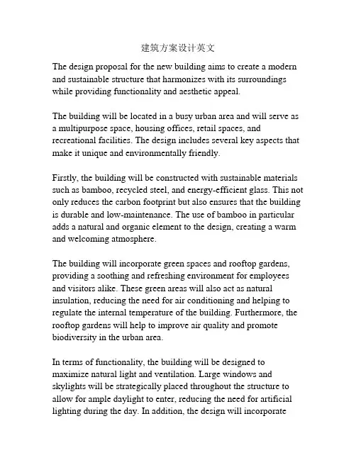
In conclusion, the design proposal for the new building aims to create a sustainable and functional structure that enhances the urban landscape and provides a pleasant and productive environment for its occupants. Through the use of sustainable materials, green spaces, and innovative design features, the building will become a landmark in the area, demonstrating the importance of sustainable architecture in creating a greener and more liveable city.
新荷塘显示器国际有限公司NHD-4.3-480272FT-CSXV-CTP 4.3英寸EVE2 TF

NHD-4.3-480272FT-CSXV-CTP4.3” EVE2 TFT Module (SPI) – Supports: Display | Touch | Audio NHD- Newhaven Display4.3- 4.3” Diagonal480272- 480xRGBx272 PixelsFT- ModelC- On-board ControllerS- High Brightness, White LED BacklightX- TFTV- Full View (MVA), Wide TemperatureCTP- Capacitive Touch PanelNewhaven Display International, Inc.2661 Galvin Ct.Elgin IL, 60124Ph: 847-844-8795 Fax: 847-844-8796Functions and Features∙ 4.3" Premium EVE2 TFT Module w/ Capacitive Touch∙On-board FTDI/Bridgetek FT813 Embedded Video Engine (EVE2)∙Supports Display, Touch, Audio∙SPI Interface (D-SPI/Q-SPI modes available)∙1MB of Internal Graphics RAM∙Built-in Scalable Fonts∙24-bit True Color, 480x272 Resolution (WQVGA)∙Supports Portrait and Landscape modes∙High Brightness (700 cd/m²)∙On-board ON Semiconductor FAN5333BSX High Efficiency LED Driver w/ PWM ∙4x Mounting Holes, enabling standard M3 or #6-32 screws∙Open-Source Hardware, Engineered in Elgin, IL (USA)[read caution below]CN2: FFC Connector - 20-Pin, 1.0mm pitch, Top-contact.NOTICE: It is not recommended to apply power to the board without a display connected. Doing so may result in a damaged LED driver circuit. Newhaven Display does not assume responsibility for failures due to this damage. Controller InformationThis EVE2 TFT Module is powered by the FTDI/Bridgetek FT813 Embedded Video Engine (EVE2).To view the full FT81x specification, please download it by accessing the link below:/Support/Documents/DataSheets/ICs/DS_FT81x.pdfThis product consists of the above TFT display assembled with a PCB which supports all the features of this module. For more details on the TFT display itself, please download the specification at:/specs/NHD-4.3-480272EF-ASXV-CTP.pdfArduino ApplicationIf using or prototyping this EVE2 TFT Module with the low-cost, widely popular Arduino platform we highly recommend using our Arduino shield, the NHD-FT81x-SHIELD. Not only does the NHD-FT81x-SHIELD provide seamless connectivity and direct software compatibility for the user, but it also comes with the following useful features on-board: ∙logic level shifters to allow the 5V Arduino to communicate with the 3.3V FT81x∙regulators to allow the Arduino to output more current to the EVE2 TFT Module∙audio filter/amplifier circuit to utilize the EVE2 TFT Module’s audio output signal∙microSD card slot, which allows expandable storage for data such as images, video, and audio to be stored. Please visit the NHD-FT81x-SHIELD product webpage for more info.Backlight Driver ConfigurationThe Backlight Driver Enable signal is connected to the FT81x backlight control pin. This signal is controlled by two registers: REG_PWM_HZ and REG_PWM_DUTY. REG_PWM_HZ specifies the PWM output frequency – the range available on the FT81x is 250 to 10000Hz, however the on-board backlight driver’s max PWM frequency is 1000Hz. Therefore, for proper use of the PWM function available on this module, the PWM frequency should not exceed 1000Hz. REG_PWM_DUTY specifies the duty cycle – the range is 0 to 128. A value of 0 turns the backlight completely off, while a value of 128 provides maximum backlight brightness.For the above register definitions, please refer to pages 80-81 of the official FT81x Series Programmers Guide:/Support/Documents/ProgramGuides/FT81X_Series_Programmer_Guide.pdfFT81x Block DiagramFT81x with EVE (Embedded Video Engine) technology simplifies the system architecture for advanced Human Machine Interfaces (HMIs) by providing support for display, touch, and audio as well as an object oriented architecture approach that extends from display creation to the rendering of the graphics.Serial Host InterfaceBy default the SPI slave operates in the SINGLE channel mode with MOSI as input from the master and MISO as output to the master. DUAL and QUAD channel modes can be configured through the SPI slave itself. To change the channel modes, write to register REG_SPI_WIDTH. Please refer to the table below:For more details on the FT81x SPI interface, please refer to pages 13-15 of the official FT81x Datasheet:/Support/Documents/DataSheets/ICs/DS_FT81x.pdfFor the REG_SPI_WIDTH register definition, please refer to page 87 of the official FT81x Series Programmers Guide: /Support/Documents/ProgramGuides/FT81X_Series_Programmer_Guide.pdfTFT Timing CharacteristicsShown below are the FT81x registers that control the TFT’s timing (clock and sync signals), along with the values recommended to use for this EVE2 TFT Module:Graphics EngineThe graphics engine executes the display list once for every horizontal line. It executes the primitive objects in the display list and constructs the display line buffer. The horizontal pixel content in the line buffer is updated if the object is visible at the horizontal line.Main features of the graphics engine are:∙The primitive objects supported by the graphics processor are: lines, points, rectangles, bitmaps (comprehensive set of formats), text display, plotting bar graph, edge strips, and line strips, etc.∙Operations such as stencil test, alpha blending and masking are useful for creating a rich set of effects such as shadows, transitions, reveals, fades and wipes.∙Anti-aliasing of the primitive objects (except bitmaps) gives a smoothing effect to the viewer.∙Bitmap transformations enable operations such as translate, scale and rotate.∙Display pixels are plotted with 1/16th pixel precision.∙Four levels of graphics states∙Tag buffer detectionThe graphics engine also supports customized built-in widgets and functionalities such as jpeg decode, screen saver, calibration etc. The graphics engine interprets commands from the MPU host via a 4 Kbyte FIFO in the FT81x memory at RAM_CMD. The MPU/MCU writes commands into the FIFO, and the graphics engine reads and executes the commands. The MPU/MCU updates the register REG_CMD_WRITE to indicate that there are new commands in the FIFO, and the graphics engine updates REG_CMD_READ after commands have been executed.Main features supported are:∙Drawing of widgets such as buttons, clock, keys, gauges, text displays, progress bars, sliders, toggle switches, dials, gradients, etc.∙JPEG and motion-JPEG decode∙Inflate functionality (zlib inflate is supported)∙Timed interrupt (generate an interrupt to the host processor after a specified number of milliseconds)∙In-built animated functionalities such as displaying logo, calibration, spinner, screen saver and sketch∙Snapshot feature to capture the current graphics displayFor a complete list of graphics engine display commands and widgets, please refer to Chapter 4 of the officialFT81x Series Programmers Guide:/Support/Documents/ProgramGuides/FT81X_Series_Programmer_Guide.pdfTouch-Screen EngineThe Capacitive Touch Screen Engine (CTSE) of the FT813 communicates with the external Capacitive Touch Panel Module (CTPM) through an I2C interface. The CTPM will assert its interrupt line when there is a touch detected. Upon detecting CTP_INT_N line active, the FT813 will read the touch data through I2C. Up to 5 touches can be reported and stored in FT813 registers.For more details on the FT813 Touch-Screen Engine, please refer to pages 32-35 of the official FT81x Datasheet:/Support/Documents/DataSheets/ICs/DS_FT81x.pdfAudio EngineThe FT81x provides mono audio output through a PWM output pin, AUDIO_L. It outputs two audio sources, the sound synthesizer and audio file playback.This pin is designed to be passed into a simple filter circuit and then passed to an amplifier for best results. Please refer to the example schematic in the Audio Filter and Amplifier Reference Circuit section on the next page.Sound SynthesizerA sound processor, AUDIO ENGINE, generates the sound effects from a small ROM library of waves table. To play a sound effect listed in Table 4.3, load the REG_SOUND register with a code value and write 1 to the REG_PLAY register. The REG_PLAY register reads 1 while the effect is playing and returns a ‘0’ when the effect ends. Some sound effects play continuously until interrupted or instructed to play the next sound effect. To interrupt an effect, write a new value to REG_SOUND and REG_PLAY registers; e.g. write 0 (Silence) to REG_SOUND and 1 to PEG_PLAY to stop the sound effect.The sound volume is controlled by register REG_VOL_SOUND. The 16-bit REG_SOUND register takes an 8-bit sound in the low byte. For some sounds, marked "pitch adjust" in the table below, the high 8 bits contain a MIDI note value. For these sounds, a note value of zero indicates middle C. For other sounds the high byte of REG_SOUND is ignored. Audio PlaybackThe FT81x can play back recorded sound through its audio output. To do this, load the original sound data into theFT81x’s RAM, and set r egisters to start the playback. The registers controlling audio playback are:REG_PLAYBACK_START: The start address of the audio data.REG_PLAYBACK_LENGTH: The length of the audio data, in bytes.REG_PLAYBACK_FREQ: The playback sampling frequency, in Hz.REG_PLAYBACK_FORMAT: The playback format, one of LINEAR SAMPLES, uLAW SAMPLES, orADPCM SAMPLES.REG_PLAYBACK_LOOP: If ‘0’, the sample is played once. If ‘1’, the sample is repeated indefinitely.REG_PLAYBACK_PLAY: A write to this location triggers the start of audio playback, regardless ofwriting ‘0’ or ‘1’. Read back ‘1’when playback is ongoing, and ‘0’ whenplayback finishes.REG_VOL_PB: Playback volume, 0-255.The mono audio formats supported are 8-bits PCM, 8-bits uLAW and 4-bits IMA-ADPCM. For ADPCM_SAMPLES, each sample is 4 bits, so two samples are packed per byte, the first sample is in bits 0-3 and the second is in bits 4-7.The current audio playback read pointer can be queried by reading the REG_PLAYBACK_READPTR. Using a large sample buffer, looping, and this read pointer, the host MPU/MCU can supply a continuous stream of audio.For more details on the FT81x Audio Engine, please refer to pages 30-32 of the official FT81x Datasheet:/Support/Documents/DataSheets/ICs/DS_FT81x.pdfAdditional Information/ResourcesFT81x Datasheet:FTDI/Bridgetek FT81x Embedded Video Engine (EVE2)/Support/Documents/DataSheets/ICs/DS_FT81x.pdfProgrammers Guide:FT81x Series Programmers Guide/Support/Documents/ProgramGuides/FT81X_Series_Programmer_Guide.pdfNHD GitHub Page:NHD EVE2 TFT Module Example Projectshttps:///NewhavenDisplay/EVE2-TFT-ModulesEVE2 Software Examples:FT81x Example Projects/Support/SoftwareExamples/FT800_Projects.htmFTDI/Bridgetek Utilities:Screen Designer/Support/Utilities.htm#ESD3Image Converters/Support/Utilities.htm#EVEImageConvertersAudio Converter/Support/Utilities.htm#EVEAudioConverterFont Converter/Support/Utilities.htm#EVEFontConverterFT80x to FT81x Migration Guide:FT80x to FT81x Migration Guide/Support/Documents/AppNotes/AN_390%20FT80x%20To%20FT81x%20Migration%20Guide.pdfNote 2: Conducted after 4 hours of storage at 25⁰C, 0%RH.Note 3:Test performed on product itself, not inside a container.Precautions for using LCDs/LCMsSee Precautions at /specs/precautions.pdfWarranty InformationSee Terms & Conditions at /index.php?main_page=terms。
BloxOne
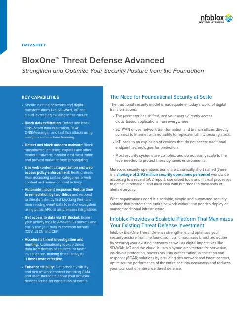
DATASHEETBloxOne™ Threat Defense AdvancedStrengthen and Optimize Your Security Posture from the FoundationThe Need for Foundational Security at ScaleThe traditional security model is inadequate in today’s world of digitaltransformations.• The perimeter has shifted, and your users directly accesscloud-based applications from everywhere.• SD-WAN drives network transformation and branch offices directlyconnect to Internet with no ability to replicate full HQ security stack.• IoT leads to an explosion of devices that do not accept traditionalendpoint technologies for protection.• Most security systems are complex, and do not easily scale to thelevel needed to protect these dynamic environments.Moreover, security operations teams are chronically short staffed (thereis a shortage of 2.93 million security operations personnel worldwideaccording to a recent ISC2 report), use siloed tools and manual processesto gather information, and must deal with hundreds to thousands ofalerts everyday.What organizations need is a scalable, simple and automated securitysolution that protects the entire network without the need to deploy ormanage additional infrastructure.Infoblox Provides a Scalable Platform That MaximizesYour Existing Threat Defense InvestmentInfoblox BloxOne Threat Defense strengthens and optimizes yoursecurity posture from the foundation up. It maximizes brand protectionby securing your existing networks as well as digital imperatives likeSD-WAN, IoT and the cloud. It uses a hybrid architecture for pervasive,inside-out protection, powers security orchestration, automation andresponse (SOAR) solutions by providing rich network and threat context,optimizes the performance of the entire security ecosystem and reducesyour total cost of enterprise threat defense.Figure 2: BloxOne ThreatMaximize Security Operation Center EfficiencyReduce Incident Response Time• Automatically block malicious activity and provide the threat data to the rest of your security ecosystem for investigation, quarantine and remediation• Optimize your SOAR solution using contextual network and threat intelligence data, and Infoblox ecosystem integrations (a critical enabler of SOAR)-reduce threat response time and OPEX• Reduce number of alerts to review and the noise from your firewallsUnify Security Policy with Threat Intel Portability • Collect and manage curated threat intelligence data from internal and external sources and distribute it to existing security systemsAdvanced Threat DetectionSOARNetwork Access Control(NAC)Next-Gen Endpoint Security• Reduce cost of threat feeds while improving effectiveness of threat intel across entire security portfolio Faster Threat Investigation and Hunting• Makes your threat analysts team 3x more productive by empowering security analysts with automated threat investigation, insights into related threats and additional research perspectives from expert cyber sources to make quick, accurate decisions on threats. • Reduce human analytical capital neededFigure 1: Infoblox hybrid architecture enables protection everywhere and deployment anywhereInfoblox is leading the way to next-level DDI with its Secure Cloud-Managed Network Services. Infoblox brings next-level security, reliability and automation to on-premises, cloud and hybrid networks, setting customers on a path to a single pane of glass for network management. Infoblox is a recognized leader with 50 percent market share comprised of 8,000 customers, including 350 of the Fortune 500.Corporate Headquarters | 3111 Coronado Dr. | Santa Clara, CA | 95054+1.408.986.4000 | 1.866.463.6256 (toll-free, U.S. and Canada) | ***************** | © 2019 Infoblox, Inc. All rights reserved. Infoblox logo, and other marks appearing herein are property of Infoblox, Inc. All other marks are the property of their respective owner(s).Hybrid Approach Protects Wherever You areDeployedAnalytics in the Cloud• Leverage greater processing capabilities of the cloud to detect a wider range of threats, including data exfiltration, domain generation algorithm (DGA), fast flux, fileless malware, Dictionary DGA and more using machine learning based analytics• Detect threats in the cloud and enforce anywhere to protect HQ, datacenter, remote offices or roaming devices Threat Intelligence Scaling• Apply comprehensive intelligence from Infoblox research and third-party providers to enforce policies on-premises or in the cloud, and automatically distribute it to the rest of the security infrastructure• Apply more threat intelligence in the cloud without huge investments into more security appliances for every sitePowerful integrations with your security ecosystem • Enables full integration with on-premises Infoblox and third-party security technologies, enabling network-wide remediation and improving ROI of those technologies Remote survivability/resiliency• If there is ever a disruption in your Internet connectivity, the on-premises Infoblox can continue to secure the networkTo learn more about the ways that BloxOne Threat Defense secures your data and infrastructure, please visit: https:///products/bloxone-threat-defense“In this day and age there is way too muchransomware, spyware, and adware coming in over links opened by Internet users. The Infoblox cloud security solution helps block users from redirects that take them to bad sites, keeps machines from becoming infected, and keeps users safer.”Senior System Administrator and Network Engineer,City University of Seattle。
三层方案解析英文
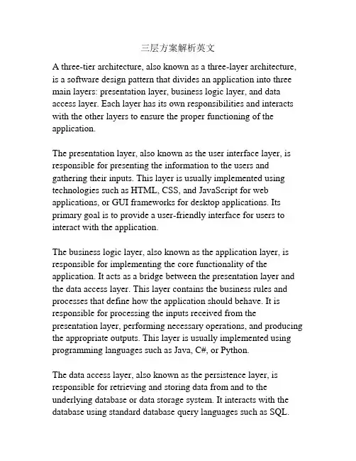
三层方案解析英文A three-tier architecture, also known as a three-layer architecture, is a software design pattern that divides an application into three main layers: presentation layer, business logic layer, and data access layer. Each layer has its own responsibilities and interacts with the other layers to ensure the proper functioning of the application.The presentation layer, also known as the user interface layer, is responsible for presenting the information to the users and gathering their inputs. This layer is usually implemented using technologies such as HTML, CSS, and JavaScript for web applications, or GUI frameworks for desktop applications. Its primary goal is to provide a user-friendly interface for users to interact with the application.The business logic layer, also known as the application layer, is responsible for implementing the core functionality of the application. It acts as a bridge between the presentation layer and the data access layer. This layer contains the business rules and processes that define how the application should behave. It is responsible for processing the inputs received from the presentation layer, performing necessary operations, and producing the appropriate outputs. This layer is usually implemented using programming languages such as Java, C#, or Python.The data access layer, also known as the persistence layer, is responsible for retrieving and storing data from and to the underlying database or data storage system. It interacts with the database using standard database query languages such as SQL.This layer allows the application to perform CRUD (Create, Read, Update, Delete) operations on the data. It abstracts the details of the underlying data storage system from the rest of the application, making it easier to switch between different types of data storage systems without affecting the other layers.One of the main advantages of the three-tier architecture is its modularity and scalability. Each layer can be developed and maintained independently, allowing teams to work on different parts of the application simultaneously. This also enables easy testing, debugging, and maintenance of the application. Additionally, the three-tier architecture allows for horizontal scaling by adding more servers to handle increased user load, without affecting the functionality of the application.Another advantage of the three-tier architecture is its flexibility. By separating the presentation layer from the business logic layer and the data access layer, it becomes possible to change or upgrade one layer without affecting the others. For example, if the presentation layer needs to be redesigned to support mobile devices, it can be done without modifying the business logic or the data access layer. However, the three-tier architecture is not without its drawbacks. The additional layers and the communication between them can introduce performance overhead. Also, the complexity of managing the interactions between the layers can increase as the application grows. Therefore, it is important to carefully design and optimize the architecture to ensure the best performance and maintainability.Overall, the three-tier architecture provides a scalable and flexible solution for developing software applications. By separating the application into distinct layers, it enables modular development, easy maintenance, and future-proofing of the application.。
如何做建筑方案设计英文术语

建筑方案设计英文术语Introduction:This architectural design proposal aims to create a cutting-edge, sustainable and visually striking building that will serve as a vibrant focal point in the city. The design will seamlessly blend functionality, aesthetics, and sustainability to create a building that will stand the test of time and make a positive impact on its surroundings. The proposed building will be located in the heart of the city, with easy access to public transportation, amenities, and green spaces.Design Concept:The design concept for this building is inspired by the concept of "organic architecture", which seeks to integrate the building with its natural surroundings in a harmonious way. The building will feature a combination of modern materials and innovative technologies, such as solar panels, green roofs, and passive heating and cooling systems, to minimize its environmental impact. The design will prioritize natural lighting, ventilation, and green spaces to create a healthy and sustainable environment for its occupants.Key Features:1. Sustainable Design: The building will be designed to achieve LEED Platinum certification, incorporating energy-efficient systems, water-saving features, and sustainable materials throughout.2. Green Roofs: The building will feature extensive green roofs, providing insulation, improving air quality, and reducing heat island effect in the city.3. Passive Design: The building will be designed to maximize natural ventilation and lighting, reducing the need for artificial heating and cooling systems.4. Flexible Spaces: The building will feature flexible spaces that can be easily adapted to accommodate a variety of uses, from office space to residential units.5. Public Amenities: The building will include public amenities such as cafes, shops, and outdoor seating areas to enhance the vibrancy of the neighborhood.Design Elements:1. Facade: The building's facade will feature a combination of glass, steel, and sustainable wood panels, creating a dynamic and modern aesthetic.2. Atrium: The building will feature an expansive atrium with a green wall, creating a sense of connection to nature within the building.3. Rooftop Terrace: The building will include a rooftop terrace with panoramic views of the city skyline, providing a relaxing space for occupants to unwind and socialize.4. Courtyard: The building will include a central courtyard with lush landscaping, creating a tranquil retreat for building occupants.5. Community Spaces: The building will include community spaces such as a fitness center, meeting rooms, and event spaces, fostering a sense of community among building occupants. Conclusion:This architectural design proposal aims to create a building that not only meets the functional needs of its occupants but also responds to the environmental and social challenges of our time. By prioritizing sustainability, aesthetics, and community, this building will set a new standard for urban architecture and serve as a model for future developments. We look forward to working with you to bring this design to life and create a building that makes a positive impact on the city and its residents.。
wuji3
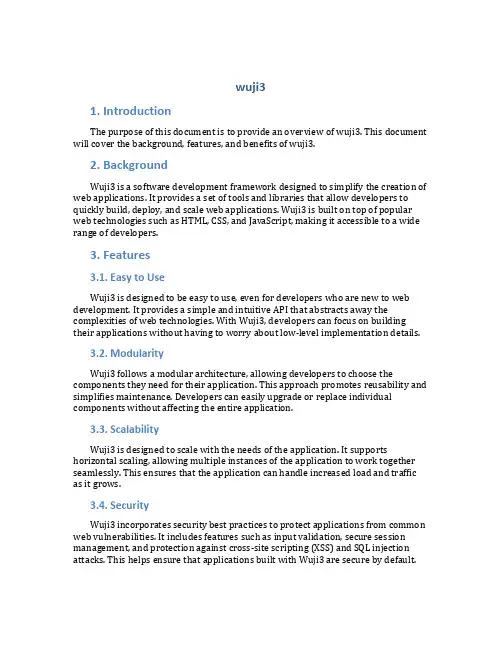
wuji31. IntroductionThe purpose of this document is to provide an overview of wuji3. This document will cover the background, features, and benefits of wuji3.2. BackgroundWuji3 is a software development framework designed to simplify the creation of web applications. It provides a set of tools and libraries that allow developers to quickly build, deploy, and scale web applications. Wuji3 is built on top of popular web technologies such as HTML, CSS, and JavaScript, making it accessible to a wide range of developers.3. Features3.1. Easy to UseWuji3 is designed to be easy to use, even for developers who are new to web development. It provides a simple and intuitive API that abstracts away the complexities of web technologies. With Wuji3, developers can focus on building their applications without having to worry about low-level implementation details.3.2. ModularityWuji3 follows a modular architecture, allowing developers to choose the components they need for their application. This approach promotes reusability and simplifies maintenance. Developers can easily upgrade or replace individual components without affecting the entire application.3.3. ScalabilityWuji3 is designed to scale with the needs of the application. It supports horizontal scaling, allowing multiple instances of the application to work together seamlessly. This ensures that the application can handle increased load and traffic as it grows.3.4. SecurityWuji3 incorporates security best practices to protect applications from common web vulnerabilities. It includes features such as input validation, secure session management, and protection against cross-site scripting (XSS) and SQL injection attacks. This helps ensure that applications built with Wuji3 are secure by default.3.5. ExtensibilityWuji3 provides a robust plugin system that allows developers to extend the functionality of their applications. Developers can easily integrate third-party libraries or develop their own plugins to add new features or enhance existing ones.4. BenefitsThere are several benefits of using Wuji3 for web application development: •Reduced development time: Wuji3 simplifies the development process, allowing developers to build applications faster.•Increased productivity: With its easy-to-use API and modular architecture, Wuji3 enables developers to work more efficiently.•Improved scalability: Wuji3’s scalable architecture ensures that applications can handle increased demand without sacrificing performance.•Enhanced security: Wuji3 incorporates security best practices, providing a more secure environment for web applications.•Flexibility: The extensibility of Wuji3 allows developers to customize and enhance their applications according to their specific needs.5. ConclusionIn conclusion, Wuji3 is a powerful framework that simplifies web application development. With its easy-to-use API, modular architecture, scalability, security features, and extensibility, Wuji3 provides a robust foundation for building modern web applications. Whether you are a beginner or an experienced developer, Wuji3 can help you create web applications more efficiently and securely.。
Declaration of Authorship
Efficient Hardware Architectures forModular MultiplicationbyDavid Narh AmanorA Thesissubmitted toThe University of Applied Sciences Offenburg, GermanyIn partial fulfillment of the requirements for theDegree of Master of ScienceinCommunication and Media EngineeringFebruary, 2005Approved:Prof. Dr. Angelika Erhardt Prof. Dr. Christof Paar Thesis Supervisor Thesis SupervisorDeclaration of Authorship“I declare in lieu of an oath that the Master thesis submitted has been produced by me without illegal help from other persons. I state that all passages which have been taken out of publications of all means or unpublished material either whole or in part, in words or ideas, have been marked as quotations in the relevant passage. I also confirm that the quotes included show the extent of the original quotes and are marked as such. I know that a false declaration willhave legal consequences.”David Narh AmanorFebruary, 2005iiPrefaceThis thesis describes the research which I conducted while completing my graduate work at the University of Applied Sciences Offenburg, Germany.The work produced scalable hardware implementations of existing and newly proposed algorithms for performing modular multiplication.The work presented can be instrumental in generating interest in the hardware implementation of emerging algorithms for doing faster modular multiplication, and can also be used in future research projects at the University of Applied Sciences Offenburg, Germany, and elsewhere.Of particular interest is the integration of the new architectures into existing public-key cryptosystems such as RSA, DSA, and ECC to speed up the arithmetic.I wish to thank the following people for their unselfish support throughout the entire duration of this thesis.I would like to thank my external advisor Prof. Christof Paar for providing me with all the tools and materials needed to conduct this research. I am particularly grateful to Dipl.-Ing. Jan Pelzl, who worked with me closely, and whose constant encouragement and advice gave me the energy to overcome several problems I encountered while working on this thesis.I wish to express my deepest gratitude to my supervisor Prof. Angelika Erhardt for being in constant touch with me and for all the help and advice she gave throughout all stages of the thesis. If it was not for Prof. Erhardt, I would not have had the opportunity of doing this thesis work and therefore, I would have missed out on a very rewarding experience.I am also grateful to Dipl.-Ing. Viktor Buminov and Prof. Manfred Schimmler, whose newly proposed algorithms and corresponding architectures form the basis of my thesis work and provide the necessary theoretical material for understanding the algorithms presented in this thesis.Finally, I would like to thank my brother, Mr. Samuel Kwesi Amanor, my friend and Pastor, Josiah Kwofie, Mr. Samuel Siaw Nartey and Mr. Csaba Karasz for their diverse support which enabled me to undertake my thesis work in Bochum.iiiAbstractModular multiplication is a core operation in many public-key cryptosystems, e.g., RSA, Diffie-Hellman key agreement (DH), ElGamal, and ECC. The Montgomery multiplication algorithm [2] is considered to be the fastest algorithm to compute X*Y mod M in computers when the values of X, Y and M are large.Recently, two new algorithms for modular multiplication and their corresponding architectures were proposed in [1]. These algorithms are optimizations of the Montgomery multiplication algorithm [2] and interleaved modular multiplication algorithm [3].In this thesis, software (Java) and hardware (VHDL) implementations of the existing and newly proposed algorithms and their corresponding architectures for performing modular multiplication have been done. In summary, three different multipliers for 32, 64, 128, 256, 512, and 1024 bits were implemented, simulated, and synthesized for a Xilinx FPGA.The implementations are scalable to any precision of the input variables X, Y and M.This thesis also evaluated the performance of the multipliers in [1] by a thorough comparison of the architectures on the basis of the area-time product.This thesis finally shows that the newly optimized algorithms and their corresponding architectures in [1] require minimum hardware resources and offer faster speed of computation compared to multipliers with the original Montgomery algorithm.ivTable of Contents1Introduction 91.1 Motivation 91.2 Thesis Outline 10 2Existing Architectures for Modular Multiplication 122.1 Carry Save Adders and Redundant Representation 122.2 Complexity Model 132.3 Montgomery Multiplication Algorithm 132.4 Interleaved Modular Multiplication 163 New Architectures for Modular Multiplication 193.1 Faster Montgomery Algorithm 193.2 Optimized Interleaved Algorithm 214 Software Implementation 264.1 Implementational Issues 264.2 Java Implementation of the Algorithms 264.2.1 Imported Libraries 274.2.2 Implementation Details of the Algorithms 284.2.3 1024 Bits Test of the Implemented Algorithms 30 5Hardware Implementation 345.1 Modeling Technique 345.2 Structural Elements of Multipliers 34vTable of Contents vi5.2.1 Carry Save Adder 355.2.2 Lookup Table 375.2.3 Register 395.2.4 One-Bit Shifter 405.3 VHDL Implementational Issues 415.4 Simulation of Architectures 435.5 Synthesis 456 Results and Analysis of the Architectures 476.1 Design Statistics 476.2 Area Analysis 506.3 Timing Analysis 516.4 Area – Time (AT) Analysis 536.5 RSA Encryption Time 557 Discussion 567.1 Summary and Conclusions 567.2 Further Research 577.2.1 RAM of FPGA 577.2.2 Word Wise Multiplication 57 References 58List of Figures2.3 Architecture of the loop of Algorithm 1b [1] 163.1 Architecture of Algorithm 3 [1] 21 3.2 Inner loop of modular multiplication using carry save addition [1] 233.2 Modular multiplication with one carry save adder [1] 254.2.2 Path through the loop of Algorithm 3 29 4.2.3 A 1024 bit test of Algorithm 1b 30 4.2.3 A 1024 bit test of Algorithm 3 314.2.3 A 1024 bit test of Algorithm 5 325.2 Block diagram showing components that wereimplemented for Faster Montgomery Architecture 35 5.2.1 VHDL implementation of carry save adder 36 5.2.2 VHDL implementation of lookup table 38 5.2.3 VHDL implementation of register 39 5.2.4 Implementation of ‘Shift Right’ unit 40 5.3 32 bit blocks of registers for storing input data bits 425.4 State diagram of implemented multipliers 436.2 Percentage of configurable logic blocks occupied 50 6.2 CLB Slices versus bitlength for Fast Montgomery Multiplier 51 6.3 Minimum clock periods for all implementations 52 6.3 Absolute times for all implementations 52 6.4 Area –time product analysis 54viiList of Tables6.1 Percentage of configurable logic block slices(out of 19200) occupied depending on bitlength 47 6.1 Number of gates 48 6.1 Minimum period and maximum frequency 48 6.1 Number of Dffs or Latches 48 6.1 Number of Function Generators 49 6.1 Number of MUX CARRYs 49 6.1 Total equivalent gate count for design 49 6.3 Absolute Time (ns) for all implementations 53 6.4 Area –Time Product Values 54 6.5 Time (ns) for 1024 bit RSA encryption 55viiiChapter 1Introduction1.1 MotivationThe rising growth of data communication and electronic transactions over the internet has made security to become the most important issue over the network. To provide modern security features, public-key cryptosystems are used. The widely used algorithms for public-key cryptosystems are RSA, Diffie-Hellman key agreement (DH), the digital signature algorithm (DSA) and systems based on elliptic curve cryptography (ECC). All these algorithms have one thing in common: they operate on very huge numbers (e.g. 160 to 2048 bits). Long word lengths are necessary to provide a sufficient amount of security, but also account for the computational cost of these algorithms.By far, the most popular public-key scheme in use today is RSA [9]. The core operation for data encryption processing in RSA is modular exponentiation, which is done by a series of modular multiplications (i.e., X*Y mod M). This accounts for most of the complexity in terms of time and resources needed. Unfortunately, the large word length (e.g. 1024 or 2048 bits) makes the RSA system slow and difficult to implement. This gives reason to search for dedicated hardware solutions which compute the modular multiplications efficiently with minimum resources.The Montgomery multiplication algorithm [2] is considered to be the fastest algorithm to compute X*Y mod M in computers when the values of X, Y and M are large. Another efficient algorithm for modular multiplication is the interleaved modular multiplication algorithm [4].In this thesis, two new algorithms for modular multiplication and their corresponding architectures which were proposed in [1] are implemented. TheseIntroduction 10 algorithms are optimisations of Montgomery multiplication and interleaved modular multiplication. They are optimised with respect to area and time complexity. In both algorithms the product of two n bit integers X and Y modulo M are computed by n iterations of a simple loop. Each loop consists of one single carry save addition, a comparison of constants, and a table lookup.These new algorithms have been proved in [1] to speed-up the modular multiplication operation by at least a factor of two in comparison with all methods previously known.The main advantages offered by these new algorithms are;•faster computation time, and•area requirements and resources for the implementation of their architectures in hardware are relatively small compared to theMontgomery multiplication algorithm presented in [1, Algorithm 1a and1b].1.2 Thesis OutlineChapter 2 provides an overview of the existing algorithms and their corresponding architectures for performing modular multiplication. The necessary background knowledge which is required for understanding the algorithms, architectures, and concepts presented in the subsequent chapters is also explained. This chapter also discusses the complexity model which was used to compare the existing architectures with the newly proposed ones.In Chapter 3, a description of the new algorithms for modular multiplication and their corresponding architectures are presented. The modifications that were applied to the existing algorithms to produce the new optimized versions are also explained in this chapter.Chapter 4 covers issues on the software implementation of the algorithms presented in Chapters 2 and 3. The special classes in Java which were used in the implementation of the algorithms are mentioned. The testing of the new optimized algorithms presented in Chapter 3 using random generated input variables is also discussed.The hardware modeling technique which was used in the implementation of the multipliers is explained in Chapter 5. In this chapter, the design capture of the architectures in VHDL is presented and the simulations of the VHDLIntroduction 11 implementations are also discussed. This chapter also discusses the target technology device and synthesis results. The state machine of the implemented multipliers is also presented in this chapter.In Chapter 6, analysis and comparison of the implemented multipliers is given. The vital design statistics which were generated after place and route were tabulated and graphically represented in this chapter. Of prime importance in this chapter is the area – time (AT) analysis of the multipliers which is the complexity metric used for the comparison.Chapter 7 concludes the thesis by setting out the facts and figures of the performance of the implemented multipliers. This chapter also itemizes a list of recommendations for further research.Chapter 2Existing Architectures for Modular Multiplication2.1 Carry Save Adders and Redundant RepresentationThe core operation of most algorithms for modular multiplication is addition. There are several different methods for addition in hardware: carry ripple addition, carry select addition, carry look ahead addition and others [8]. The disadvantage of these methods is the carry propagation, which is directly proportional to the length of the operands. This is not a big problem for operands of size 32 or 64 bits but the typical operand size in cryptographic applications range from 160 to 2048 bits. The resulting delay has a significant influence on the time complexity of these adders.The carry save adder seems to be the most cost effective adder for our application. Carry save addition is a method for an addition without carry propagation. It is simply a parallel ensemble of n full-adders without any horizontal connection. Its function is to add three n -bit integers X , Y , and Z to produce two integers C and S as results such thatC + S = X + Y + Z,where C represents the carry and S the sum.The i th bit s i of the sum S and the (i + 1)st bit c i+1 of carry C are calculated using the boolean equations,001=∨∨=⊕⊕=+c z y z x y x c z y x s ii i i i i i i i i iExisting Architectures for Modular Multiplication 13 When carry save adders are used in an algorithm one uses a notation of the form (S, C) = X + Y + Zto indicate that two results are produced by the addition.The results are now represented in two binary words, an n-bit word S and an (n+1) bit word C. Of course, this representation is redundant in the sense that we can represent one value in several different ways. This redundant representation has the advantage that the arithmetic operations are fast, because there is no carry propagation. On the other hand, it brings to the fore one basic disadvantage of the carry save adder:•It does not solve our problem of adding two integers to produce a single result. Rather, it adds three integers and produces two such that the sum of these two is equal to that of the three inputs. This method may not be suitable for applications which only require the normal addition.2.2 Complexity ModelFor comparison of different algorithms we need a complexity model that allows fora realistic evaluation of time and area requirements of the considered methods. In[1], the delay of a full adder (1 time unit) is taken as a reference for the time requirement and quantifies the delay of an access to a lookup table with the same time delay of 1 time unit. The area estimation is based on empirical studies in full-custom and semi-custom layouts for adders and storage elements: The area for 1 bit in a lookup table corresponds to 1 area unit. A register cell requires 4 area units per bit and a full adder requires 8 area units. These values provide a powerful and realistic model for evaluation of area and time for most algorithms for modular multiplication.In this thesis, the percentage of configurable logic block slices occupied and the absolute time for computation are used to evaluate the algorithms. Other hardware resources such as total number of gates and number of flip-flops or latches required were also documented to provide a more practical and realistic evaluation of the algorithms in [1].2.3 Montgomery Multiplication AlgorithmThe Montgomery algorithm [1, Algorithm 1a] computes P = (X*Y* (2n)-1) mod M. The idea of Montgomery [2] is to keep the lengths of the intermediate resultsExisting Architectures for Modular Multiplication14smaller than n +1 bits. This is achieved by interleaving the computations and additions of new partial products with divisions by 2; each of them reduces the bit-length of the intermediate result by one.For a detailed treatment of the Montgomery algorithm, the reader is referred to [2] and [1].The key concepts of the Montgomery algorithm [1, Algorithm 1b] are the following:• Adding a multiple of M to the intermediate result does not change the valueof the final result; because the result is computed modulo M . M is an odd number.• After each addition in the inner loop the least significant bit (LSB) of theintermediate result is inspected. If it is 1, i.e., the intermediate result is odd, we add M to make it even. This even number can be divided by 2 without remainder. This division by 2 reduces the intermediate result to n +1 bits again.• After n steps these divisions add up to one division by 2n .The Montgomery algorithm is very easy to implement since it operates least significant bit first and does not require any comparisons. A modification of Algorithm 1a with carry save adders is given in [1, Algorithm 1b]:Algorithm 1a: Montgomery multiplication [1]P-M;:M) then P ) if (P (; }P div ) P :(*M; p P ) P :(*Y; x P ) P :() {n; i ; i ) for (i (;) P :(;: LSB of P p bit of X;: i x X;in bits of n: number M ) ) (X*Y(Output: P MX, Y Y, M with Inputs: X,i th i -n =≥=+=+=++<===<≤625430201 mod 20001Existing Architectures for Modular Multiplication15Algorithm 1b: Fast Montgomery multiplication [1]P-M;:M) then P ) if (P (C;S ) P :(;} C div ; C :S div ) S :(*M; s C S :) S,C (*Y; x C S :) S,C () {n; i ; i ) for (i (; ; C : ) S :(;: LSB of S s bit of X;: i x X;of bits in n: number M ) ) (X*Y(Output: P M X, Y Y, M with Inputs: X,i th i -n =≥+===++=++=++<====<≤762254302001mod 20001In this algorithm the delay of one pass through the loop is reduced from O (n ) to O (1). This remarkable improvement of the propagation delay inside the loop of Algorithm 1b is due to the use of carry save adders to implement step (3) and (4) in Algorithm 1a.Step (3) and (4) in Algorithm 1b represent carry save adders. S and C denote the sum and carry of the three input operands respectively.Of course, the additions in step (6) and (7) are conventional additions. But since they are performed only once while the additions in the loop are performed n times this is subdominant with respect to the time complexity.Figure 1 shows the architecture for the implementation of the loop of Algorithm 1b. The layout comprises of two carry save adders (CSA) and registers for storing the intermediate results of the sum and carry. The carry save adders are the dominant occupiers of area in hardware especially for very large values of n (e.g. n 1024).In Chapter 3, we shall see the changes that were made in [1] to reduce the number of carry save adders in Figure1 from 2 to 1, thereby saving considerable hardware space. However, these changes also brought about other area consuming blocks such as lookup tables for storing precomputed values before the start of the loop.Existing Architectures for Modular Multiplication 16Fig. 1: Architecture of the loop of algorithm 1b [1].There are various modifications to the Montgomery algorithm in [5], [6] and [7]. All these algorithms aimed at decreasing the operating time for faster system performance and reducing the chip area for practical hardware implementation. 2.4 Interleaved Modular MultiplicationAnother well known algorithm for modular multiplication is the interleaved modular multiplication. The details of the method are sketched in [3, 4]. The idea is to interleave multiplication and reduction such that the intermediate results are kept as short as possible.As shown in [1, Algorithm 2], the computation of P requires n steps and at each step we perform the following operations:Existing Architectures for Modular Multiplication17• A left shift: 2*P• A partial product computation: x i * Y• An addition: 2*P+ x i * Y •At most 2 subtractions:If (P M) Then P := P – M; If (P M) Then P := P – M;The partial product computation and left shift operations are easily performed by using an array of AND gates and wiring respectively. The difficult task is the addition operation, which must be performed fast. This was done using carry save adders in [1, Algorithm 4], introducing only O (1) delay per step.Algorithm 2: Standard interleaved modulo multiplication [1]P-M; }:M) then P ) if (P (P-M; :M) then P ) if (P (I;P ) P :(*Y; x ) I :(*P; ) P :() {i ; i ; n ) for (i (;) P :( bit of X;: i x X;of bits in n: number M X*Y Output: P M X, Y Y, M with Inputs: X,i th i =≥=≥+===−−≥−===<≤765423 0 1201mod 0The main advantages of Algorithm 2 compared to the separated multiplication and division are the following:• Only one loop is required for the whole operation.• The intermediate results are never any longer than n +2 bits (thus reducingthe area for registers and full adders).But there are some disadvantages as well:Existing Architectures for Modular Multiplication 18 •The algorithm requires three additions with carry propagation in steps (5),(6) and (7).•In order to perform the comparisons in steps (4) and (5), the preceding additions have to be completed. This is important for the latency because the operands are large and, therefore, the carry propagation has a significant influence on the latency.•The comparison in step (6) and (7) also requires the inspection of the full bit lengths of the operands in the worst case. In contrast to addition, the comparison is performed MSB first. Therefore, these two operations cannot be pipelined without delay.Many researchers have tried to address these problems, but the only solution with a constant delay in the loop is the one of [8], which has an AT- complexity of 156n2.In [1], a different approach is presented which reduces the AT-complexity for modular multiplication considerably. In Chapter 3, this new optimized algorithm is presented and discussed.Chapter 3New Architectures for Modular Multiplication The detailed treatment of the new algorithms and their corresponding architectures presented in this chapter can be found in [1]. In this chapter, a summary of these algorithms and architectures is given. They have been designed to meet the core requirements of most modern devices: small chip area and low power consumption.3.1 Faster Montgomery AlgorithmIn Figure 1, the layout for the implementation of the loop of Algorithm 1b consists of two carry save adders. For large wordsizes (e.g. n = 1024 or higher), this would require considerable hardware resources to implement the architecture of Algorithm 1b. The motivation behind this optimized algorithm is that of reducing the chip area for practical hardware implementation of Algorithm 1b. This is possible if we can precompute the four possible values to be added to the intermediate result within the loop of Algorithm 1b, thereby reducing the number of carry save adders from 2 to 1. There are four possible scenarios:•if the sum of the old values of S and C is an even number, and if the actual bit x i of X is 0, then we add 0 before we perform the reduction of S and C by division by 2.•if the sum of the old values of S and C is an odd number, and if the actual bit x i of X is 0, then we must add M to make the intermediate result even.Afterwards, we divide S and C by 2.•if the sum of the old values of S and C is an even number, and if the actual bit x i of X is 1, but the increment x i *Y is even, too, then we do not need to add M to make the intermediate result even. Thus, in the loop we add Y before we perform the reduction of S and C by division by 2. The same action is necessary if the sum of S and C is odd, and if the actual bit x i of X is 1 and Y is odd as well. In this case, S+C+Y is an even number, too.New Architectures for Modular Multiplication20• if the sum of the old values of S and C is odd, the actual bit x i of X is 1, butthe increment x i *Y is even, then we must add Y and M to make the intermediate result even. Thus, in the loop we add Y +M before we perform the reduction of S and C by division by 2.The same action is necessary if the sum of S and C is even, and the actual bit x i of X is 1, and Y is odd. In this case, S +C +Y +M is an even number, too.The computation of Y +M can be done prior to the loop. This saves one of the two additions which are replaced by the choice of the right operand to be added to the old values of S and C . Algorithm 3 is a modification of Montgomery’s method which takes advantage of this idea.The advantage of Algorithm 3 in comparison to Algorithm 1 can be seen in the implementation of the loop of Algorithm 3 in Figure 2. The possible values of I are stored in a lookup-table, which is addressed by the actual values of x i , y 0, s 0 and c 0. The operations in the loop are now reduced to one table lookup and one carry save addition. Both these activities can be performed concurrently. Note that the shift right operations that implement the division by 2 can be done by routing.Algorithm 3: Faster Montgomery multiplication [1]P-M;:M) then P ) if (P (C;S ) P :(;} C div ; C :S div ) S :(I;C S :) S,C ( R;) then I :) and x y c ((s ) if ( Y;) then I :) and x y c (not(s ) if ( M;) then I :x ) and not c ((s ) if (; ) then I :x ) and not c ((s ) if () {n; i ; i ) for (i (; ; C : ) S :(M; of Y uted value R: precomp ;: LSB of Y , y : LSB of C , c : LSB of S s bit of X;: i x X;of bits in n: number M ) ) (X*Y(Output: P M X, Y Y, M with Inputs: X,i i i i th i -n =≥+===++==⊕⊕=⊕⊕=≠==++<===+=<≤10922876540302001mod 2000000000000001New Architectures for Modular Multiplication 21Fig. 2: Architecture of Algorithm 3 [1]In [1], the proof of Algorithm 3 is presented and the assumptions which were made in arriving at an Area-Time (AT) complexity of 96n2 are shown.3.2 Optimized Interleaved AlgorithmThe new algorithm [1, Algorithm 4] is an optimisation of the interleaved modular multiplication [1, Algorithm 2]. In [1], four details of Algorithm 2 were modified in order to overcome the problems mentioned in Chapter 2:•The intermediate results are no longer compared to M (as in steps (6) and(7) of Algorithm 2). Rather, a comparison to k*2n(k=0... 6) is performedwhich can be done in constant time. This comparison is done implicitly in the mod-operation in step (13) of Algorithm 4.New Architectures for Modular Multiplication22• Subtractions in steps (6), (7) of Algorithm 2 are replaced by one subtractionof k *2n which can be done in constant time by bit masking. • Next, the value of k *2n mod M is added in order to generate the correctintermediate result (step (12) of Algorithm 4).• Finally, carry save adders are used to perform the additions inside the loop,thereby reducing the latency to a constant. The intermediate results are in redundant form, coded in two words S and C instead of generated one word P .These changes made by the authors in [1] led to Algorithm 4, which looks more complicated than Algorithm 2. Its main advantage is the fact that all the computations in the loop can be performed in constant time. Hence, the time complexity of the whole algorithm is reduced to O(n ), provided the values of k *2n mod M are precomputed before execution of the loop.Algorithm 4: Modular multiplication using carry save addition [1]M;C) (S ) P :(M;})*C *C S *S () A :( A);CSA(S, C,) :) (S,C ( I); CSA(S, C,C) :) (S,(*Y;x ) I :(*A;) A :(*C;) C :(*S;) S :(; C ) C :(; S ) S :() {; i ; i n ) for (i (; ; A : ; C :) S :( bit of X;: i x X;of bits in n: number M X*Y Output: P MX, Y Y, M with Inputs: X,n n n n n i n n th i mod 12mod 2221110982726252mod 42mod 30120001mod 011+=+++=========−−≥−=====<≤++New Architectures for Modular Multiplication 23Fig. 3: Inner loop of modular multiplication using carry save addition [1]In [1], the authors specified some modifications that can be applied to Algorithm 2 in order simplify and significantly speed up the operations inside the loop. The mathematical proof which confirms the correctness of the Algorithm 4 can be referred to in [1].The architecture for the implementation of the loop of Algorithm 4 can be seen in the hardware layout in Figure 3.In [1], the authors showed how to reduce both area and time by further exploiting precalculation of values in a lookup-table and thus saving one carry save adder. The basic idea is:。
javaweb英文参考文献
javaweb英文参考文献下面是关于JavaWeb的参考文献的相关参考内容,字数超过了500字:1. Banic, Z., & Zrncic, M. (2013). Modern Java EE Design Patterns: Building Scalable Architecture for Sustainable Enterprise Development. Birmingham, UK: Packt Publishing Ltd. This book provides an in-depth exploration of Java EE design patterns for building scalable and sustainable enterprise applications using JavaWeb technologies.2. Sharma, S., & Sharma, R. K. (2017). Java Web Services: Up and Running. Sebastopol, CA: O'Reilly Media. This book provides a comprehensive guide to building Java Web services using industry-standard technologies like SOAP, REST, and XML-RPC.3. Liang, Y. D. (2017). Introduction to Java Programming: Brief Version, 11th Edition. Boston, MA: Pearson Education. This textbook introduces Java programming concepts and techniques, including JavaWeb development, in a concise and easy-to-understand manner. It covers topics such as servlets, JSP, and JavaServer Faces.4. Ambler, S. W. (2011). Agile Modeling: Effective Practices for Extreme Programming and the Unified Process. Hoboken, NJ: John Wiley & Sons. This book discusses agile modeling techniques for effective JavaWeb development, including iterative and incremental development, test-driven development, and refactoring.5. Bergeron, D. (2012). Java and XML For Dummies. Hoboken, NJ: John Wiley & Sons. This beginner-friendly book provides an introduction to using XML in JavaWeb development, covering topics such as XML parsing, JAXB, and XML Web services.6. Cadenhead, R. L., & Lemay, L. (2016). Sams Teach Yourself Java in 21 Days, 8th Edition. Indianapolis, IN: Sams Publishing. This book offers a step-by-step approach to learning Java, including JavaWeb development. It covers important topics such as servlets, JSP, and JavaServer Faces.7. Balderas, F., Johnson, S., & Wall, K. (2013). JavaServer Faces: Introduction by Example. San Francisco, CA: Apress. This book provides a practical introduction to JavaServer Faces (JSF), a web application framework for building JavaWeb user interfaces. It includes numerous examples and case studies.8. DeSanno, N., & Link, M. (2014). Beginning JavaWeb Development. New York, NY: Apress. This book serves as a comprehensive guide to JavaWeb development, covering topics such as servlets, JSP, JavaServer Faces, and JDBC.9. Murach, J. (2014). Murach's Java Servlets and JSP, 3rd Edition. Fresno, CA: Mike Murach & Associates. This book provides a deep dive into Java servlets and JSP, two core technologies for JavaWeb development. It includes practical examples and exercises.10. Horstmann, C. (2018). Core Java Volume II--AdvancedFeatures, 11th Edition. New York, NY: Prentice Hall. This book covers advanced topics in Java programming, including JavaWeb development using technologies such as servlets, JSP, JSTL, and JSF.These references cover a wide range of topics related to JavaWeb development, from introductory to advanced concepts. They provide valuable insights, examples, and practical guidance for developers interested in building web applications using Java technologies.。
罗克威尔自动化与以太网 IP技术:连接工厂网络的多种选项说明书
Stratix 5900 Camera CameraIn this illustration, both lines have the same private IP addresses (ControlLogix-192.168.1.3, Point I/O-192.168.1.4, PanelView Plus 6-192.168.1.5) on their respective local control network. This allows the lines to be exact duplicates of each other, reducing development and support time. For those nodes that need to communicate to the public plant network (ControlLogix and PanelView Plus 6) the NAT mapping functionality in each of the three products shown allows these nodes to appear as a node on the plant network.For example, if a Server PC on the public plant network (IP 172.16.10.1) needs tocommunicate to the ControlLogix on Line 1, it sees that ControlLogix as being on the public plant network at 172.16.10.13Only the local control network nodes you select to map are accessable from the public plant network. The Point I/O is not accessable in this illustration.NAT IllustrationStratix 5700 with NAT Applications requiring managed switch plus NAT capability 9300-ENAApplications with Embedded or Unmanaged SwitchesCamera Camera In this illustration, the plant wishes to segment nodes on each of the two physical networks (Assembly Line 1 & 2) into 4 logical networks (VLANs 10, 20, 30, 40). This is to isolate devices for functional and/or traffic considerations.The Stratix 5700 Layer 2 switch supports creating these VLANs.VLAN 10 has a ControlLogix, it’s Point I/O and a PanelView Plus 6. VLAN 20 has the same. These networks are isolated from each other.VLAN 30 has a Supervisory Controller PC – again isolated from the others VLAN (10 or 20 and 40) networks are on the same cable.VLAN 40 illustrates another key advantage of VLANs. It contains streamingvideo cameras used for remote machine diagnostic support. These generate a lot of traffic, but since they are on a separate VLAN they have no impact on the local traffic of VLANs 10 & 20 or PC VLAN 30.If a device on one VLAN needs to communicate to another (the SupervisoryController PC needs to communicate to the Assembly Line 1 ControlLogix), the level 3 routing capability in the Stratix 8300 Layer 30 switch supports setting up this VLAN 30 to VLAN 10 link.VLAN IllustrationCatalog #Description1783-BMS10CL Stratix 5700 Layer 2 Managed Switch, 10 Ports 1783-RMS10T Stratix 8300 Layer 3 Managed Switch, 10 Ports 1783-MS10T Stratix 8000 Layer 2 Managed Switch, 10 Ports 1783-SR Stratix 5900 Security Appliance1756-EN2TSC ControlLogix Secure Communications Module 9300-ENA Ethernet Network Appliance1783-US08TStratix 2000 Unmanaged Switch, 8 PortsAdditional ResourcesENET-PP005B-EN-E Stratix 5700 Industrial Ethernet Switch Product Profile ENET-UM003A-EN-P 1756-EN2TSC EtherNet/IP Secure Communication User ManualENET-AT004B-EN-E Segmentation Methods within the Cell / Area Zone ENET-WP025-EN-E Scalable Secure Remote Access Solutions for OEMs ENET-WP031A-EN-E Design Considerations for Securing Industrial AutomationENET-TD001-EN-P Converged Plantwide Ethernet (CPwE) Design and Implementation Guide (DIG)ENET-QR001-EN-E Stratix Switch Reference Chart ENET-QR002-EN-E Stratix 5700 Reference ChartGMSP-PP001-EN-E 9300-ENA Network Address Translation Device Product Profile SECUR-AT001A-EN-EIndustrial Security Best PracticesPublic Plant Network802.1x Security - An IEEE standard for access control and authentication. It can be used to track access to network resources and helps secure the network infrastructure.ACLs (Access Control Lists) - allow you to filter network traffic. This can be used to selectively block types of traffic to provide traffic flow control or provide a basic level of security for accessing your network.IPSec (IP Security) - A framework of open standards that provides data confidentiality, data integrity, and data authentication between participating peers.Firewall - Asecurity system that controls the incoming and outgoing network traffic by analyzing the data packets and determining whether they should be allowed through or not, based on a rule set. A firewall establishes a barrier between a trusted, secure internal network and another network (e.g., the Internet) that is not assumed to be secure and trusted.Unified Threat Management (UTM) - An evolution of the traditional firewall into an all-inclusive security product that has the ability to perform multiple security functions in one single appliance: network firewalling, network intrusion prevention and gateway antivirus (AV), gateway anti-spam, VPN, content filtering, load balancing, data leak prevention and on-appliance reporting.VPN (Virtual Private Network) - A network that uses primarily public telecommunication infrastructure, such as the Internet, to provide remote users an access to a central organizational network. VPNs typically require remote users of the network to be authenticated, and often secure data with encryption technologies.Reference Architecture Web Page/rockwellautomation/products-technologies/network-technology/architectures.page。
贝塔波特 —— 按需循环建筑技术 BetaP
建筑设计特别嘉许奖 Special Recognition in Architectural Design36 WORLD ARCHITECTURE REVIEW 建筑时空ARCHITECTURE NOWBetaPort 是由空间创新工作室Urban Beta 发明和设计的,工作室不断创造包容、非传统和变革性的空间,采用参与式方法开发空间系统。
BetaPort 本身则是一种经过认证的专利建筑技术。
每个元素都在工厂进行测试和质量检查,以保证产品质量。
在现场,所有元件都可以快速轻松地组装。
除此以外,BetaPort 也提供了适配的配置器使设计变得简单且具有成本效益,为循环经济提供了变革性的项目开发与可持续建筑技术。
缺乏生活空间、空间效率、可持续性等的城市挑战需要新的、以需求为导向的整体方法,Urban Beta 的工作即是涉及社会正义、预测性规划、共同创造和设计民主化的探索与尝试。
Betaport Providing Scalable Building Solutions for a Circular Future BetaPort provides circular "Building As a Service" (BAaS) solutions for sustainable architectures on-demand. We offer adaptive spaces that are flexible in use and follow an open-source mentality. Our system can grow over time and adapt to future use cases, activated through predictive planning for maximum efficient layouts. BetaPort offers the seamless integration of technical solutions as well as a circular production chain, including material tracking. Sustainable Architecture, digitally planned, using Automation The BetaPort system is built upon highly flexible interior layouts, based on modular, reversible building blocks.The design can react to changes, like varying capacities or alternating functions. BetaPort comes with its own digital planning tool: The BetaPort configurator. It serves as an interactive platform to connect various project stakeholders, decision makers, planners and users alike. Using machine learning and custom algorithms the configurator is designed for playful and efficient planning. It eliminates planning errors , anticipates building costs and creates production data. Affordable and Easy to Build BetaPort construction has a certified and patented building technology with a streamlined production. Every element is tested and quality checked in the factory to guarantee a great product. On site all elements are easy to assemble, by skilled and non-skilled workers. BetaPort fosters the democratization of construction through its participatory, systematic and open-source approach to building. We offer digital manuals for all building scales and sizes, including custom elements. Completely designed on Circular Economy Principles Designed for disassembly: BetaPort uses material passport and reversible connections. Completely designed from renewables or cycled materials BetaPort aims to provide sustainable buildings that create carbon sinks and active material depots. Innovative material sourcing and combination strategies allow for upcycled and secondary materials in the construction system. In this way BetaPort enables new business models, based on space on-demand solutions, service and subscription models to create "Buildings as a Service" (BaaS).BetaPort ONE BetaPort One is the world's first circular hub on-demand, completely implemented with our efficient planning process and our ecological building system. BetaPort One seamlessly integrates innovative mobility solutions and charging infrastructure into a new generation mobility hub: circular, sustainable, participatory planned and easy to scale. With our circular design approach, every BetaPort ONE pop-up becomes an actively managed material depot including material passports. Thanks to an ecosystem of components, rooms can easily be added, relocated or remodeled. Relocation to other locations is possible ina short time thanks to the simple construction system.BetaPort– Circular Building Technology On-Demand贝塔波特 —— 按需循环建筑技术建筑设计:Urban Beta UGDesign Company: Urban Beta UGCopyright ©博看网. All Rights Reserved.。
- 1、下载文档前请自行甄别文档内容的完整性,平台不提供额外的编辑、内容补充、找答案等附加服务。
- 2、"仅部分预览"的文档,不可在线预览部分如存在完整性等问题,可反馈申请退款(可完整预览的文档不适用该条件!)。
- 3、如文档侵犯您的权益,请联系客服反馈,我们会尽快为您处理(人工客服工作时间:9:00-18:30)。
Scalable Architecture for Providing Per-flow Bandwidth Guarantees Vasil Hnatyshin1 and Adarshpal S. Sethi21Department of Computer Science Rowan University201 Mullica Hill Rd.Glassboro, NJ 08028hnatyshin@2Department of Computer and InformationSciences,University of Delaware,Newark, DE 19716sethi@ ABSTRACTDespite numerous efforts, the problem of providing per-flow Quality of Service in a scalable manner still remains an active area of research. This paper introduces a scalable architecture for support of per-flow bandwidth guarantees, called the Bandwidth Distribution Scheme (BDS). The BDS maintains aggregate flow information in the network core and distributes this information among boundary nodes as needed. Based on the feedback from the network core the boundary nodes dynamically adjust resource allocations of individual flows. The BDS architecture consists of three main components: the admission control, the resource distribution mechanism, and the protocol for distributing the aggregate flow requirements in the network. This paper describes components of the BDS architecture and illustrates how they operate together to achieve scalable per-flow QoS.Keywords: Quality of service, bandwidth distribution, network feedback, resource allocation1.INTRODUCTIONTo solve the problem of providing scalable per-flow Quality of Service, a number of service differentiation models have been proposed. The Integrated and Differentiated Service (DiffServ) models are among the most prominent approaches to providing Quality of Service in the Internet. The Integrated Services model [2]requires each router in the network to reserve and manage resources for the flows that travel through it. In large networks, millions of flows may simultaneously travel through the same core routers. In such cases, managing resource reservations on a per-flow basis may cause enormous processing and storage overheads in the core routers. As a result, the Integrated Services model is considered to be not scalable to large networks and thus is not widely deployed in the Internet. The DiffServ model [1]attempts to solve the scalability problem of the Integrated Services approach by combining flows that have similar quality of service requirements into traffic aggregates or classes. The DS core routers process incoming traffic based on the class the packets belong to and thus maintain and manage resource reservations only on a per-class/per-aggregate basis. The DiffServ approach provides a scalable solution to the QoS problem but it supports only coarse per-aggregate guarantees which in certain cases may not be adequate.This paper examines the architecture of an alternative approach, called the Bandwidth Distribution Scheme (BDS). The BDS core routers do not maintain per-flow information (e.g. bandwidth requirements of individual flows); instead core routers keep aggregate flow requirements. The amount of information kept in the network core is proportional not to the number of flows but to the number of edge routers, which we believe does not raise scalability concerns. The edge nodes maintain per-flow information and fairly allocate network resources (e.g. bandwidth) among individual flows according to the flow requirements and resource availability. The dynamic resource allocation at the edge routers is enabled by the network feedback which consists of periodic path probing and explicit congestion notifications. Overall, the BDS architecture consists of: the admission control mechanism, which determines if a new flow can be admitted into the network, the resource allocation mechanism, which fairly distributes available bandwidth among individual flows, and the protocol for distribution of the aggregate flow requirements, which provides feedback to the network routers about the changes of network characteristics.The BDS approach relies on the basic idea of performing per-flow management at the network edges and processing traffic aggregates in the network core. This idea is not new and has been examined before, for instance in [1,12,15,16]. However, the primary contribution of this work is a novel approach to aggregating flow information in the network core, dynamically distributing it among edge nodes, and then using the aggregate flow requirements for fair distribution of available bandwidth among individual flows.The rest of the paper is organized as follows. Section 2 presents an overview of the BDS architecture. Section 3 introduces specification of flow requirements and the admission control mechanism. Definitions of fairness and the resource management mechanism are presented in Section 4, while Section 5 discusses the BDS network architecture and the protocol for dynamic distribution of aggregate flow requirements. Section 6 discusses implementation issues of the Bandwidth Distribution Scheme, while Section 7 provides an example of the BDSoperation. Finally, discussion and conclusions are presented in Sections 8 and 9 respectively.2. THE OVERVIEW OF THE BDS ARCHITECTURE The BDS architecture provides a scalable solution to the problems of fair per-flow bandwidth distribution and congestion control. This architecture consists of three components and a set of specifications and definitions. The BDS components are: per-flow admission control which denies access into the network for those flows that violate existing per-flow guarantees, per-flow resource allocation which dynamically distributes available bandwidth among individual flows, and the Requested Bandwidth Range Distribution (RBR) and Feedback protocol which distributes aggregate flow requirements and generates congestion notifications. The BDS specifications and definitions consist of the network architecture which defines the working environment of the BDS and makes the proposed solutions scalable to large networks, definition of the flow requirements which outlines the format for user expectations for traffic treatment, and definitions of fairness which specify what it means for the resource distribution to be fair. The BDS components along with the BDS specifications and definitions form the architecture of the Bandwidth Distribution Scheme as shown in Figure 1.Figure 1. The BDS architectureIn the BDS architecture each BDS component is closely connected to a particular specification or definition as shown in Figure 1. For example, the BDS admission controldetermines if a new flow can enter the network based on the provided specification of flow requirements, while the BDS resource allocation mechanism distributes bandwidth among individual flows based on provided definitions of fairness. That is why, in subsequent sections, we introduce the BDS components together with their corresponding BDS specifications and definitions.This paper defines a "flow" to be a sequence of packets that travel from a given source host to a given destinationhost. We only consider the flows that receive the BDS treatment and which are therefore subject to the BDS resource allocation. Similarly, the terms “resources”, “capacity”, “load,” or “bandwidth” mean the resources, bandwidth, etc. explicitly allocated by the network administrator for the BDS traffic. This definition of a flow, while different from the more conventional definition as a sequence of packets between individual source-destination applications (e.g., TCP or UDP streams), was chosen to simplify the presentation of the BDS scheme. The BDS architecture, as presented here, can be easily extended to apply to the conventional definition of a flow.3. DEFINITION OF FLOW REQUIREMENTS ANDADMISSION CONTROLIn this paper we assume that both the minimum and the maximum transmission rates of a flow are known ahead of time. Thus, the flow requirements are defined in the form of a range which is called the Requested Bandwidth Range (RBR). The RBR of flowf , f RBR , consists of twovalues: a minimum rate, fb , below which the flow cannot operate normally, and the maximum rate,fB , that the flow can utilize.],[f f f B b RBR =(1)Based on this definition, the BDS network guarantees that each flow would receive at least its minimum requested rate,f b , while the leftover resources in the network are fairlydistributed among participating flows. To achieve these guarantees, the network allocates to each flow an amount of bandwidth not smaller than the flow’s minimum requested rate, and denies network access to those flows whose minimum rate guarantees cannot be met.The purpose of admission control is to determine if a new flow can be admitted into the network at its minimum rate without violating existing QoS guarantees of other flows. The problem of admission control was extensively examined in the literature [3, 4, 8]. Traditionally, there are two types of admission control: parameter-based and measurement-based . In parameter-based admission control, the decision to admit a new flow is derived from the parameters of the flow specification. Usually, this type of admission control relies on worst-case bounds and results in low network utilization, although it does guarantee supported quality of service. Measurement-based admission control relies on measurements of the existing traffic characteristics to make the control decision. Measurement-based admission control supports higher network utilization. However, measurement-based admission control may occasionally cause the quality of service levels to drop below user expectations because of its inability to accurately predict future traffic behavior. Since the network guarantees that each flow will receive at least its minimum requested rate, the edge nodes should check the current resource allocation on a path before granting a new flow request. Thus, to admit a new flow intoScalability Fair Per-flowBandwidth Distribution Congestion ControlBDS Goals BDS Architecturethe network, the edge routers verify that the sum of the minimum requested rates of all the flows that follow a particular path, including a new flow, is smaller than the capacity of the bottleneck link on that path. Link k is a bottleneck link for flow f traveling on path P if k limits the transmission rate of f on P .We formally define the BDS admission control as follows. Consider a network consisting of a set of L unidirectional links, where link 1 L k ∈ has capacity kC . The network is shared by the set of flows, F , where flow F f ∈ has the RBR of ],[f fB b . At any time, the flow transmits packetsat a ratef R , called the allocated rate , which lies betweenf b and f B . Let L L f ⊆ denote the set of links traversed by flow f on its way to the destination. Also letF F k⊆denote the set of flows that traverse link k . Thena new flow φ with the RBR of ],[φφB b is accepted in thenetwork if and only if:k Ff fC bb k≤+∑∈φ φL k ∈∀(2)Thus, a new flow, φ, is accepted into the network only if the sum of the minimum requested rates of the active flows, including the new flow, is not larger than the capacity of each link on the path of flow φ to the destination. Equation (2) is often called the admission control test .4. DEFINITIONS OF FAIRNESS AND THERESOURCE ALLOCATION MECHANISMIn this section we introduce two definitions of fairness, examine and compare the ability of these definitions to maximize network throughput, and introduce the BDS resource allocation mechanism that fairly distributes available bandwidth among individual flows based on introduced definitions of fairness.4.1. Definitions of FairnessConsider a core router’s interface k and a set of flows, kF ,that travel through it. The setkF can be divided into two disjoint subsets: the subset, kB F , of flows that have link kas their bottleneck and the subset, kNB F , that contain all theother flows. These subsets are called bottleneck flows and non-bottleneck flows , respectively.U kNB k B k F F F =(3)The aggregate bottleneck RBR and the aggregate RBR on interface k are defined as follows:1In this paper the terms link, interface, and interface to a link are often used interchangeably.∑∈=kBF f fk B bb ∑∈=kBF f fk B BB (4) ∑∈=kF f fk bb∑∈=kF f fk BB(5)The aggregate bottleneck RBR is the sum of the RBRs of the bottleneck flows on link k , while the aggregate RBR is the sum of the RBRs of all the flows that travel through link k . The total allocated rate of the non-bottleneck flows is called the non-bottleneck rate and is denoted as kNB R . The amount of bandwidth left for distribution among the bottleneck flows is the difference between the capacity of link k and the non-bottleneck rate. This value is called the bottleneck capacity, kB C .k NBF f k fk kBR C RC C k NB∑∈−=−= (6)When a link is not fully utilized, its bottleneck capacity could be larger then the sum of the allocated rates of the bottleneck flows. Table 1 provides a summary of the presented definitions.Table 1. Summary of the traffic type definitions for fairness specificationFlowsRBRCapacityAll flows:U k NBkBkFFF = Aggregate RBR: ∑∈=kF f f kb b ∑∈=kF f fkB BLink Capacity:kNBk B k R R C +=∑∈≥kF f fk RC Bottleneck flows: kNBk k B F F F −= AggregateBottleneck RBR: ∑∈=kBF f f k B b b ∑∈=k BF f fkBBBBottleneckCapacity:k NB k k B R C C −= ∑∈≥kb F f fK B RCNon-bottleneck Flows:kB kk NB F F F −= AggregateNon-bottleneck RBR:Not used, not defined.Non-bottleneck Rate:∑∈=kNBF f fkNBRRk Bkk NBC C R−≤Based on the notation specified in Table 1, we introduce two definitions of fairness. First, the proportional fair share,k f FS , of the flow f on link k is defined as follows:k bfk B k B f k Bk Bfkfb b C b b b C b FS =−+=)( (7)Using definition (7), each flow is allocated its minimum requested rate plus a share of leftover bandwidth. We call this definition of fairness proportional fairness because each flow receives an amount of bandwidth proportional to itsminimum requested rate. This definition of fairness should not be confused with Kelly’s proportional fairness [8, 9], which deals with different issues. Throughout the rest of this paper, the expression “proportional fairness” refers to the definition of fairness specified by equation (7).A second definition of fairness uses a similar idea, except that the excess bandwidth is distributed proportionally to the difference between the flow’s maximum and minimum requested rates. The idea is to allocate resources proportionally to the amount of bandwidth a flow needs to be completely utilized. We assume that a flow is completely utilized when it sends traffic at its maximum requested rate,f B . That is why this definition of fairness is calledmaximizing utility fairness . The maximizing utility fair share, kf FS , of flow f on link k is computed as follows:()kBkB ff k B k B f k f b B b B b C b FS −−−+= (8)4.2. Maximizing Allocated Rate in the Network viaDefinitions of FairnessThis section examines if resource distribution using the proposed definitions of fairness achieves our primary objective of maximizing allocated rate in the network. The network has allocated rate maximized if the allocated rate on every bottleneck link is maximized. Allocated rate on a link is the sum of allocated rates of those flows that travel through that link. Thus, the allocated rate on the bottleneck link is maximized if the bottleneck capacity on that link is completely distributed among the bottleneck flows. Also, the bottleneck link has its allocated rate maximized if all the bottleneck flows that travel through that link are allocated and transmit at their maximum requested rates.Let us consider an example of Figure 2, where each link is provisioned with 48 Kbps of bandwidth. The RBR and path for each active flow are shown in Table 2, while the aggregate RBR is recorded next to the link as shown in Figure 2.Figure 2. Example of the resource distributionThe network of Figure 2 contains two bottleneck links:B1-C1 and C2-B2. Link C2-B2 is the bottleneck for flows F1, F2, and F4. The bottleneck capacity of C2-B2 equals the link’s capacity because all the flows that travel through link C2-B2 are bottleneck flows. Table 2 presents the resource distribution using both definitions of fairness. As Table 2shows, the proportional definition of fairness does not utilize all available bandwidth on link C2-B2. In particular, using the proportional fairness only 45 Kbps out of 48 Kbps of the bottleneck link’s capacity is distributed among the flows, leaving 3 Kbps of bandwidth unused. At the same time, flows F1 and F4 are sending traffic below their maximum requested rates and can utilize leftover bandwidth. Link B1-C1 is also underutilized; however, since the bottleneck flow F3 is allocated its maximum requested rate, the allocated rate on the link B1-C1 is maximized.On the other hand, the maximizing utility fairness completely distributes all available resources among the flows and keeps bottleneck link C2-B2 fully utilized. When using maximizing utility definition of fairness, link B1-C1 also remains underutilized. However, as before, the allocated rate on B1-C1 is maximized.Table 2. Example of the resource distributionFlow Flow RBR Path Proportional Fair ShareF1 [8, 14] B1-C1-C2-B2 MIN (48*(8/32), 14) = 12 F2 [10,12] B1-C1-C2-B2 MIN (48*(10/32), 12) = 12 F3 [14, 18] B1-C1-C3-B3 MIN (24*(14/14), 18) = 18 F4 [14, 22] B4-C3-C2-B2MIN (48*(14/32), 22) = 21Flow Flow RBR Path Maximizing UtilityFair ShareF1 [8, 14] B1-C1-C2-B2 MIN (8+16*6/16, 14) = 14 F2 [10,12] B1-C1-C2-B2 MIN (10+16*2/16, 12) = 12 F3 [14, 18] B1-C1-C3-B3 MIN (14+(48-26)*4/4, 18) = 18 F4 [14, 22]B4-C3-C2-B2MIN (14+16*10/16, 22) = 22Now let us examine the conditions when the proportional and the maximizing utility definitions of fairness are unable to maximize allocated rate on the bottleneck link. The link's allocated rate is maximized in two cases:1. The bottleneck flows are transmitted at theirmaximum requested rates. In this case the link's capacity may not be fully utilized.2. The bottleneck capacity is completely distributedamong the bottleneck flows. In this case the link's capacity is fully utilized.To identify the conditions when the allocated rate on the link is not maximized, we need to examine when the sum of allocated rates of the bottleneck flows is smaller than the corresponding bottleneck capacity.()∑∑∈∈<=k BfB F f kB F f f k f k fC B FSR,min(9)To determine when inequality (9) holds, we consider the following three cases:Case 1: The fair shares of all the bottleneck flows are largerthan their corresponding maximum requested rates and thus, all the bottleneck flows are allocated their maximum requested rate. Although the link is underutilized, its allocated rate is maximized because the bottleneck flows are allocated their maximum requested rates. This case corresponds to the situation on link B1-C1 of Figure 2.Case 2: All the bottleneck flows are allocated the rates thatcorrespond to their fair shares. The sum of the allocated rates of the bottleneck flows on a link equals the bottleneck capacity of that link. In this case the link capacity is completely utilized and the allocated rate on the link is maximized.Case 3: Among the bottleneck flows that travel through thelink there are flows that are allocated their maximum requested rates because their fair shares are larger than their corresponding maximum requested rates and there are flows that are allocated only their fair shares. The flows that transmit data at their maximum rates but below their fair shares cause the link to become underutilized. This case corresponds to the situation on link C2-B2 described in the example of Figure 2.Let us examine the last case for both definitions of fairness in more detail. Using proportional fairness, Case 3 yields the following inequality:f f k k B fk fk B bB b R B b b R >⇒>(10)Thus, the proportional fairness does not maximize the allocated rate on the link whenever the ratio between the bottleneck capacity and the minimum requested rate of the aggregate RBR is smaller than the ratio between the flow’s maximum and minimum requested rates. The main reason for this phenomenon is the fact that the proportional fairness does not consider the maximum requested rates in the computation of the fair shares. The maximizing utility fairness, on the other hand, does include the maximum requested rates in computation of the fair shares and thus does not suffer from the above deficiency.⇒>−−−+f kk ff kkBfB bB b B b R b )( ()⇒−>−−−ff f f kk k k B b B b B b B b R ⇒−>−k k k k B b B b R k k B B R >(11)According to inequality (11) the maximizing utility fairness causes the link to become underutilized only when the bottleneck capacity is larger than the maximum requested rate of the aggregate RBR. However, this means that all the bottleneck flows transmit traffic at their maximum requested rates and thus the allocated rate on the link is maximized.In summary, the maximizing utility fairness is able to maximize allocated rate in the network, while the proportional fairness fails to do that whenever the inequality (10) holds, and thus, may require additional mechanisms to improve the overall performance in the network.4.3. The Resource Management MechanismTo distribute bandwidth according to equations (7) – (8), the resource management mechanism requires the knowledge of such link characteristics as the aggregatebottleneck RBR and the bottleneck capacity. However, thesecharacteristics are not readily available in the network. Instead the core routers keep track of the capacity, the arrival rate, and the aggregate RBR for each outgoing link and distribute this information among the edge nodes. The edge nodes use the aggregate RBR and link capacity instead of the aggregate bottleneck RBR and the bottleneck capacity to compute fair shares of individual flows. The edge nodes compute the fair share of flow f on its bottleneck link k using the proportional and maximizing utility definitions of fairness as shown below. However, the flows that do not have link k as their bottleneck would not adjust their allocated rates.k fk k f kkfk fb b C b b b C b FS =−+=)( (12) ()k kff k k f k f b B b B b C b FS −−−+=(13)Clearly, such resource distribution may leave link k underutilized because the non-bottleneck flows will transmit data at rates below their fair shares on link k . Thus, the edge nodes require additional means for utilizing the leftover resources. A “water-filling” technique employed for implementation of the max-min fairness [13, 17] allows the edge nodes to completely distribute leftover capacity. The idea of the “water-filling” is to increase allocated rates of individual flows as long as the bottleneck link is not fully utilized.Periodic path probing, that delivers information about availability of resources on the path, enables the edge routers to implement the “water-filling” technique. Thus, in the presence of excess bandwidth the edge routers increase allocated rates of individual flows until available bandwidth on the path is consumed completely. It was shown in [5] that by distributing leftover bandwidth proportionally to the individual flow requirements the resource management mechanism achieves an optimal resource distribution defined by equations (7) – (8).The resource management mechanism enforces resource allocation through the token bucket. Thus, if a flow transmits data above its allocated rate then the token bucket discards all excess traffic of that flow. As a result, the flow injects the amount of data into the network that corresponds to its share of the allocated resources.5. THE BDS NETWORK ARCHITECTURE ANDTHE RBR DISTRIBUTION AND FEEDBACK PROTOCOL5.1. The BDS Network ArchitectureThe Internet consists of a large number of routers that are traditionally grouped into independent network domains as shown in Figure 3. A cluster of interconnected routers that are governed by the same administrator are called a network domain . Each network domain contains two types of nodes:the edge or boundary routers and the core routers. Traffic enters a network domain through the edge nodes called ingress routers. It further travels through the core routers to reach the network boundary and exits the domain through the edge nodes called egress routers.Figure 3. The BDS Network ArchitectureThe BDS core routers do not perform per-flow management and treat arriving traffic on per-aggregate basis, in a way similar to that of the Differentiated Services nodes [1]. The BDS core routers provide feedback to the boundary nodes about the changes of network conditions. The edge nodes maintain per-flow information and manage activation and termination of the flows. Based on the provided feedback the edge nodes compute the fair shares of bandwidth for their flows and then allocate available resources accordingly.It is reasonable to assume that the number of active flows that enter and exit the network domain through a particular edge router is fairly small. Thus, managing per-flow information at the network boundaries allows this network architecture to scale well to large networks [1]. Furthermore, this architecture does not require the BDS approach to be set-up everywhere in the Internet at once. Instead, each network domain can choose to support the Bandwidth Distribution Scheme at its own discretion, and thus facilitates incremental deployment of the BDS architecture in the Internet. If a network domain decides to support the BDS, then a certain amount of resources are allocated for the BDS traffic. These resources are fairly distributed among the BDS flows only, thus isolating the BDS traffic from the rest of the non-BDS flows traveling through this domain. This paper examines the architecture of the Bandwidth Distribution Scheme within the confines of a single network domain. We plan to address the issue of inter-domain traffic and deployment of the BDS approach in the Internet in future work.5.2.The RBR Distribution and Feedback (RDF) Protocol The feedback protocol that governs the information sharing between the nodes in the BDS network is called the RBR Distribution and Feedback (RDF) protocol. The RDF protocol is one of the most important components of the BDS. The RDF protocol operates as the “glue” that holds the BDS architecture together by supplying information to the admission control and the resource management mechanism. The RBR Distribution and Feedback protocol consists of two major components that determine its name: distribution of the aggregate RBR and periodic feedback from the network.The RBR Distribution and Feedback protocol consists of three distinct phases: the path probing phase, the RBR update phase, and the notification phase. Each phase is classified based on the information flow as either edge-to-core or core-to-edge. During the edge-to-core phases, the information travels from the edge nodes into the network core to update the aggregate flow requirements stored in the Interfaces Tables. At the same time, during the core-to-edge phases, information about the status of the network core is being distributed among the edge routers to refresh network information stored in the Path and the Link Tables.The path probing phase discovers characteristics of a particular path and works as follows. The ingress node periodically generates a probe message on a path while the egress node sends the probe message with collected path characteristics back to the ingress node. The ingress node uses received information to update its Path and Link Tables. In addition, the core routers can discover the edge nodes that send traffic through their interfaces using the path probing phase. For example, upon the probe message arrival, the core routers retrieve the identity of the edge node that generated this probe and update corresponding edge node entry in the Interfaces Table, which contains the identity of the edge router and a countdown timer. If the entry in the Interfaces Table for this edge router already exists, then the core node resets the corresponding countdown timer. Otherwise, the core router creates a new entry for this edge router. The core router discards the edge node's information whenever the countdown timer expires.The purpose of the RBR update phase is to notify the core routers about the changes to the aggregate RBR information upon flow activation or termination. The edge routers initiate the RBR update phase by generating the RBR update message on a particular path. Each core router renews its Interfaces Table based on the information received from the RBR update message. The egress node terminates progress of the RBR update message.Only in the event of congestion do the core routers initiate the notification phase. In this case, the core routers generate congestion notification messages to the edge routers asking them to adjust allocated rates of their flows. The edge routers update their Path and Link Tables and re-compute the fair shares of the corresponding flows based on the information received from the congestion notification messages.Thus, the edge routers update the Path and Link Tables based on the feedback received during the path probing and the notification phases, while the core routers update their Interfaces Tables during the RBR change and the path probing phases. Table 4 provides a summary and classification of the RDF protocol phases.。