ANSYS Polyflow R150 P3 Update
ANSYS_CFD之Flotran中文讲解说明
第三步: 生成有限元网格
用户必须事先确定流场中哪个地方流体的梯度变化较大,在这些地方,网格必须 作适当的调整。例如:如果用了紊流模型,靠近壁面的区域的网格密度必须比层流模 型密得多,如果太粗,该网格就不能在求解中捕捉到由于巨大的变化梯度对流动造成 的显著影响,相反,那些长边与低梯度方向一致的单元可以有很大的长宽比。 为了得到精确的结果,应使用映射网格划分,因其能在边界上更好地保持恒定的 网格特性, 映射网格划分可由命令 MSHKEY,1 或其相应的菜单 Main Menu>Preproce ssor > -Meshing-Mesh>-entity-Mapped 来实现。
FLUID141 单元
FLUID141 单元具有下列特征: 维数:二维 形状:四节点四边形或三节点三角形 自由度:速度、压力、温度、紊流动能、紊流能量耗散、多达六种流体的各自质 量所占的份额
FLUID142 单元
FLUID142 单元具有下列特征: 维数:三维 形状:四节点四面体或八节点六面体 自由度:速度、压力、温度、紊流动能、紊流能量耗散、多达六种流体的各自质 量所占的份额
FLOTRAN 分析的主要步骤
一个典型的 FLOTRAN 分析有如下七个主要步骤: 1. 确定问题的区域。 2. 确定流体的状态。 3. 生成有限元网格。 4. 施加边界条件。 5. 设置 FLOTRAN 分析参数。 6. 求解。 7. 检查结果。
第一步:确定问题的区域
用户必须确定所分析问题的明确的范围,将问题的边界设置在条件已知的地方, 如果并不知道精确的边界条件而必须作假定时,就不要将分析的边界设在靠近感兴趣 区域的地方,也不要将边界设在求解变量变化梯度大的地方。有时,也许用户并不知 道自己的问题中哪个地方梯度变化最大,这就要先作一个试探性的分析,然后再根据 结果来修改分析区域。这些在后面章节中都有详述。
ANSYS WB Meshing R150 P3 Update

2
© 2013 ANSYS, Inc.
August 9, 2013
ANSYS Confidential & Proprietary Information
Performance Robustness Usability
3
© 2013 ANSYS, Inc.
August 9, 2013
ANSYS Confidential & Proprietary Information
Offshore Oil Platform 26% Memory Reduction 7 6 5 4 3 2 1 0 14.5 15
34% Time Reduction 40 35 30 25 20 15 10 5 0 14.5 15
6
© 2013 ANSYS, Inc.
August 9, 2013
15.0 Meshing: Mesh Failure Handling
If Meshing fails, user can export mesh and edit in Fluent Meshing or ICEM CFD
16
© 2013 ANSYS, Inc.
August 9, 2013
ANSYS Confidential & Proprietary Information
11
© 2013 ANSYS, Inc.
August 9, 2013
ANSYS Confidential & Proprietary Information
Parallel part by part meshing
Parallel Part meshing
Windows Only
ANSYS ICEMCFD R150 P3 Update

8 © 2012 ANSYS, Inc. August 12, 2013
Hexa Smoothing
• Hexa smoothing development
– Increased focus on individual element quality – Improved smoothing along curves – Improved Orthogonality – New options include Post smoothing iterations with a gradient smoother
ANSYS ICEM CFD: R15.0 Update
This presentation contains ANSYS, Inc. proprietary information. It is made available to ANSYS channel partners and ANSYS customers participating in R15.0 Preview 3 Testing only. It is not to be distributed to others.
1 © 2012 ANSYS, Inc. August 12, 2013
Simon Pereira July 2013
Focus of R15
• Defect fixing was a top priority • Enhancement of ICEM CFD • Continued development of underlying technology also exposed in ANSYS Meshing
Polyflow教程3

Polyflow教程3Tutorial 3. Fluid Flow and Conjugate heat TransferIntroductionThis tutorial illustrates the setup and solution of a problem involving heat transfer between a Newtonian fluid and a cooled circular die. Along with a good die design, rheological and thermo physical properties of the melt and the thermal settings in the die are very important in obtaining a geometrically well-defined polymer product. The heat transfer calculation is important when temperature-sensitive polymers are shaped and when product surface qualities are of critical importance. The temperature field at the die exit influences the swelling and drawing behavior of the product.In this tutorial, you will solve the non-isothermal flow problem for the fluid and the heat conduction in the die, making some assumptions regarding the rheological and thermo physical properties of the melt.In this tutorial you will learn how to:Start POLYDATA from Workbench.Create a new task.Create multiple sub-tasks.Define a Newtonian non-isothermal flow problem.Define a heat conduction problem.Set material properties and boundary conditions for a fluid-solid heat conduction and flow problem.PrerequisitesThis tutorial assumes that you are familiar with the menu structure in POLYDATA and Workbench and that you have solved or read Tutorial 1. Some steps in the setup procedure will not beshown explicitly.Problem DescriptionThis tutorial examines the coupled problem of non-isothermal flow of a Newtonian fluid and heat conduction in an axisymmetric steel die. As shown in Figure 3.1, the melt enters the domain at a fixed temperature and a given flow rate of T = 180?C and Q =0.6e?06 m3/s, respectively. The problem involves flow, heat transfer by conduction and convection, and heat generation by viscous dissipation. Energy, momentum, and Fluid Flow and Conjugate heat transferincompressibility equations are solved in the fluid domain. The energy equation for heat conduction is solved in the solid domain.To solve the coupled problem, two sub-tasks are defined: one for the fluid (sub-task 1) and the other for the solid (sub-task 2). Each sub-task will contain a particular model, domain of definition, material properties, and boundary conditions, including interface conditions with the other sub-task. The sub-tasks are coupled, because the global solution of the problem depends on the values of the solution variables at the intersection of the fluid and solid domains.Figure 3.1: A Schematic Diagram of the Fluid and the Circular DieThe material properties for the fluid are:ρ = density (950 kg/m3)η = Newtonian viscosity (2500 P a s)Cp = heat capacity per unit mass (2300 J/kg-K)k = thermal conductivity (0.5 W/m-K)Viscous heating is taken into account. For the solid region, the thermal conductivity k is 35 W/m-K.Fluid Flow and Conjugate heat transfer The boundary sets for the problem are shown in Figure 3.2, and the conditions at the boundaries of the domains are:boundary 1: flow inlet, T = 180°C, Q = 0.6 × 10?6 m3/sintersection of subdomain 1 and subdomain 2: interfaceboundary 2: insulatedboundary 3: T = 100°Cboundary 4: insulatedboundary 5: flow exitboundary 6: symmetry axisFigure 3.2: Boundaries and Sub-domainsPreparation1. Copy the file, flusol/flusol.msh from the POLYFLOW documentation CD or installation area to your working directory (as described in Tutorial 1).2. Start Workbench from start?All Programs?Ansys13.0?Workbench.Fluid Flow and Conjugate heat transferStep 1: Project and Mesh1. Create a Polyflow Analysis system by drag and drop in workbench, import the meshfile (flusol.msh), and double-click the Setup cell of the analysis to start POLYDATA. Hint: For detailed information on how to do this, refer to Tutorial 1.When POLYDATA starts, the Create a new task menu item is be highlighted, and the geometry for the problem is displayed in the Graphics Display window.Step 2: Models, Material Data, and Boundary ConditionsIn this step, define a new task representing the fluid flow and conjugate heat transfer problem. The flow problem for the fluid and the heat conduction in the solid is solved in two different sub-tasks. However, the task attributes are the same for both the sub-tasks, so define a single task for the coupled problem.1. Create a task for the model.Create a new task(a) Select the following options:taskF.E.M.problemSteady-state2D axisymmetric geometrySince the problem involves an axisymmetric steel die, the computationaldomain for the problem is chosen to be a 2D cylindrical reference frame(r,z) with r=0 as the axis of symmetry, and involves two velocitycomponents (u,v); hence 2D axisymmetric geometry has been chosen. ASteady-state condition is assumed for the problem.(b) Select Accept the current setup.The Create a sub-task menu item is highlighted.Fluid Flow and Conjugate heat transferStep 2a: Definition of Sub-Task 1In this step, define the flow problem, identify the domain ofdefinition, set the relevant material properties for the Newtonian fluid, and define boundary conditions along its boundaries.1. Create the sub-task for the fluid flow.Create a sub-task(a) Select Generalized Newtonian non-isothermal flow problem.A panel appears asking for the title of the problem.(b) Enter fluid as the New value and click OK.The Domain of the sub-task menu item is highlighted.2. Define the domain where the sub-task applies.To solve the coupled problem, the computational domain is divided into two sub-domains with a common intersection. A sub-task with its own model, material properties, and boundary conditions is defined on each of the non-overlapping subdomains. Sub-task 1 is defined for Subdomain 1, since Subdomain 1 represents the fluid (as shown in Figure3.2). Domain of the sub-task(a) Select Subdomain 2 and click Remove.Fluid Flow and Conjugate heat transferSubdomain 2 is moved from the top list to the bottom list, indicating that subtask1 is defined on subdomain 1.(b) Click on Upper level menu at the top of the panel.The Material data menu item is highlighted.3. Specify the material properties for the fluid.POLYDATA indicates which material properties are relevant for your sub-task by graying out the irrelevant properties. In this sub-task, POLYFLOW solves energy, incompressibility and momentum equations, so you have to define viscosity, density, thermal conductivity, heat capacity per unit mass, and viscous heating. For a non-isothermal flow problem, the viscosity can depend on both shear rate and temperature. In this case, the viscosity is constant, so it depends on neither of them.Material data(a) Select Shear-rate dependence of viscosity.Since the fluid flow is Newtonian, specify a constant value for the viscosity.Fluid Flow and Conjugate heat transferi. Select Constant viscosity.ii. Specify the value for ηfacModifyprompts for the new value of ηPOLYDATAiii. Enter 2500 as the New value and click OK.iv. Select Upper level menu two times to continue the Material Dataspecification.(b) Select Temperature dependence of viscosity.i. Select No temperature dependence.POLYDATA displays the following message, confirming that there is notemperature dependence for the viscosity.Fluid Flow and Conjugate heat transferOK.ii.Clickiii. Select Upper level menu to continue the Material Data specification.(c) Select Density.In this problem, specify a constant value for the density.Modification of densityi. Enter 950 as the New value and click OK.ii. Select Upper level menu to continue the Material Data specification.(d) Select Thermal conductivity.Fluid Flow and Conjugate heat transfer As shown at the topof the menu, the thermal conductivity is defined as a non- linear function of the temperature:k = a + bt + ct2 + dt3(3.1) In this problem, the thermal conductivity is assumed to be a constant for the fluid, so only the constant coefficient a is modified.aModifyi. Enter 0.5 as the New value and click OK.ii. Select Upper level menu to continue the Material Data specification.(e) Select Heat capacity per unit mass.As shown at the top of the menu, the heat capacity per unit mass is defined as anon-linear function of temperature:c p = a + bt + ct2 + dt3 (3.2)The temperature variation of cp differs with the nature of the polymer melts. Inthis problem, cp is assumed to be constant, so only the constant coefficient a ismodified.Fluid Flow and Conjugate heat transferModify ai. Enter 2300 as the New value and click OK.ii. Select Upper level menu to continue the Material Data specification.(f) Select Viscous heating.When shearing occurs in a flow, the friction of the different fluid layers creates heat. When the fluid is highly viscous and/or the shear rate is high, the heating of the fluid due to this phenomenon is important and must be taken into consideration.i. Select Viscous heating will be taken into account.ii. Select Upper level menu to return to the Material Data specification.(g) Select Upper level menu to leave the Material Data specification.The Flow boundary conditions menu item is highlighted.4. Specify the flow boundary conditions for subdomain 1.Fluid Flow and Conjugate heat transfer Flow boundary conditions(a) Set the conditions along the intersection of subdomain 1 and subdomain 2.The intersection acts as a wall for the fluid, and since the fluid is assumed to stick to the wall, zero normal and tangential velocities is imposed along this boundary.i. Select Zero wall velocity (vn=vs=0) along subdomain 2 and click Modify.ii. Select Zero wall velocity (vn=vs=0).(b) Set the conditions at the flow inlet (boundary 1).i. Select Zero wall velocity (vn=vs=0) along boundary 1 and click Modify.Inflow.ii.Selectprompts for the new value of the volumetric flow rate.POLYDATAFluid Flow and Conjugate heat transferiii. Enter 0.6e-06 as the New value and click OK.The flow rate of the melt is very low due to the highly viscous nature ofthemelt.Automatic.iv.SelectWhen the Automatic option is selected, POLYDATA automatically choosesthe most appropriate method to compute the inflow condition.(c) Set the conditions at the flow exit (boundary 5).It is assumed that a fully developed velocity profile is reached at the exit, so the outflow condition is most appropriate. This condition imposes a zero normal force, f n (which includes a pressure term), and zero tangential velocity, v s.i. Select Zero wall velocity (vn=vs=0) along boundary 5 and click Modify.Outflow.ii.Select(d) Retain the default condition Axis of symmetry at thesymmetry axis(boundary 6).For axisymmetric models, POLYDATA recognizes the axis of symmetry from the mesh file, and automatically imposes the symmetry condition along the line r=0.This condition imposes a zero normal velocity vn and zero tangential force fs along this boundary.(e) Click on Upper level menu at the top of the panel to leave the Flow boundaryconditions panel.The Thermal boundary conditions menu item is highlighted.Fluid Flow and Conjugate heat transfer5. Specify the thermal boundary conditions for subdomain 1.For non-isothermal problems, specify either the temperature or the heat flux on each boundary segment. The temperature along a given boundary can be a constant or a prescribed function of coordinates.Thermal boundary conditions(a) Set the conditions at the intersection of subdomain 1 andsubdomain 2.An interface condition is set at the intersection of subdomain 1 and subdomain 2.This condition ensures continuity of the temperature field and of the heat flux along the interface. Since you are solving a coupled problem, this condition of continuity is essential for the global solution of the temperature and heat flux variables.imposedalong subdomain 2 and click Modify.TemperatureSelecti.Interface.ii.SelectFluid Flow and Conjugate heat transferiii. Select Upper level menu to accept the default setting (continuous heat flux along the interface).In the case of an interface condition, both the heat flux and temperature are usually continuous along the interface. It is possible to specify a nonzero value for the heat flux jump (dq), but this is mainly used in problems where internal radiation is simulated. Here, accept the default value for the definition of heat flux discontinuity, i.e., dq = 0.(b) Set the conditions at the flow inlet (boundary 1). A constant value for the temperature is imposed along this boundary .i. Select Temperature imposed along boundary 1 and click Modify.ii. Select Temperature imposed.iii. Select Constant. POLYDATA prompts you for the new value of the constant temperature.iv. Enter 180 as the New value and click OK. v. Select Upper level menu to return to the Thermal boundary conditions panel.(c) Set the conditions at the flow outlet (boundary 5). A zero conductive heat flux is imposed along this boundary .i. Select Temperature imposed along boundary 5 and click Modify.ii. Select Outflow.Fluid Flow and Conjugate heat transfer(d) Keep the default condition Axis of symmetry at the symmetry axis6).(boundary(e) Click on Upper level menu at the top of the Thermal boundary conditionspanel.(f) Select Upper level menu at the top of the fluid sub-task menu.Step 2b: Definition of Sub-Task 2In this step, define the heat conduction problem, identify the domain of definition, set the relevant material properties for the solid, and define the boundary conditions along its boundaries.1. Create a sub-task for the solid.Create a sub-task(a)asks if you want to copy data from an existing sub-task.POLYDATA(b) Click No, since this sub-task has different parameters associated with it.(c) Select Heat conduction problem.A small panel appears asking for the title of the problem.i. Enter solid as the New value and click OK.The Domain of the sub-task menu item is highlighted.2. Define the domain where the sub-task applies (subdomain 2).Domain of the sub-task(a) Select Subdomain 1 and click Remove.Fluid Flow and Conjugate heat transfer(b) Click on Upper level menu at the top of the panel.The Material data menu item is highlighted.3. Specify the material properties for the solid.Material dataIn this problem, specify a constant value for the thermal conductivity k.(a) Select Thermal conductivity.In this problem, thermal conductivity is assumed to be a constant, so only the constant coefficient a is modified.Fluid Flow and Conjugate heat transferi. Enter 35 as the New value and click OK.(b) Select Upper level menu two times to leave the Material Data specification.4. Specify the thermal boundary conditions for subdomain 2.In this step, set the conditions at each of the boundaries of the domain. When a boundary set is selected, it is highlighted in red in the graphics window.Thermal boundary conditions(a) Set the conditions at the intersection of subdomain 1 and subdomain 2.An interface condition is set at the intersection of the sub-domains.imposedalong subdomain 1 and click Modify.SelectTemperaturei.Interface.ii.Selectiii. Select Upper level menu to accept the default option for continuity offlux.heattemperatureand(b) Set the conditions at the bottom boundary of the solid (boundary 2).A zero conductive heat flux is imposed along this boundary.imposed along boundary 2 and click Modify.TemperatureSelecti.ii. Select Insulated boundary / symmetry.(c) Set the conditions at the outer boundary of the solid (boundary 3).Fluid Flow and Conjugate heat transferA constant value for the temperature is imposed along this boundary.Temperatureimposed along boundary 3 and click Modify.Selecti.imposed.TemperatureSelectii.SelectConstant.iii.prompts you for the new value of the constant temperature. POLYDATAiv. Enter 100 as the New value and click OK.v. Select Upper level menu to return to the Thermal boundary conditions panel.(d) Set the conditions at the top boundary of the solid (boundary 4).A zero conductive heat flux is imposed along this boundary.Temperatureimposed along boundary 4 and click Modify.Selecti.ii. Select Insulated boundary / symmetry.(e) Click on Upper level menu to leave the Thermal boundary conditions panel.(f) Select Upper level menu two times to return to the top-level POLYDATA menu.Step 3: Save the Data and Exit POLYDATAAfter defining your model in POLYDATA, save the data file. In the next step, read this data file into POLYFLOW and calculate a solution.Save and exitPOLYDATA asks you to confirm the current system units and fields that are to be saved to the results file for post-processing.1. Select Upper level menuThis confirms that the default units are correct.Fluid Flow and Conjugate heat transfer2. Select Accept.This confirms that the default Current field(s) are correct.3. Select Continue.This accepts the default names for graphical output files (cfx.res) that are to be saved for postprocessing, and the POLYFLOW format results file (res).Step 4: SolutionRun POLYFLOW to calculate a solution for the model you just defined using POLYDATA.1. Run POLYFLOW by righ click on Solution cell of the simulation and click on Update button.This executes POLYFLOW using the data file as standard input, and writes information about the problem description,calculations, and convergence to a listing file (listingFile).2. Check for convergence in the listing file.Right click on Solution cell and click on Listing Viewer…Workbench opens View listing file panel, which displays the listing file.Step 5: Post-processingUse CFDPost to view the results of the POLYFLOW simulation.1. Double click on Results cell in the workbench analysis and read the results files saved by POLYFLOW.CFDPost reads the solution fields that were saved to the results file.2. Align the view.。
ANSYS软件平台最新更新介绍
ANSYS AIM Pro
• Solvers: Fluids, Mechanical, 2 HPC • PrepPost: Workbench, SCDM, MeshingUpda源自ed Product Licenses
• Updated licenses will be announced by letter
Overset mesh can speed and simplify simulations with multiple moving parts. This example includes multiple background and component meshes.
Flow with Interacting Bodies and Arbitrary Motion
Pushing Performance Further
Problem
• Ever larger simulations!
Solution
• New scalability record 172K cores • >10X faster HDF write performance
– 20X faster than non-HDF
• Added support for
– Rotating machinery – Conjugate Heat Transfer (CHT)
• Improved solution stability
– Suppression option for dissipation stabilization scheme
Temperature, compared with experimental data
polyflow教程1
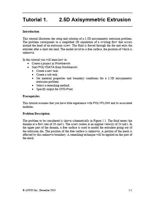
Tutorial 1. 2.5D Axisymmetric ExtrusionIntroductionThis tutorial illustrates the setup and solution of a 2.5D axisymmetric extrusion problem. The problem corresponds to a simplified 2D simulation of a swirling flow that occurs around the head of an extrusion screw. The fluid is forced through the die and exits the extruder after a short die land. The model involves a free surface, the position of which is unknown.In this tutorial you will learn how to:•Create a project in Workbench.•Start POLYDATA from Workbench.•Create a new task.•Create a sub-task.•Set material properties and boundary conditions for a 2.5D axisymmetric extrusion problem.•Select a remeshing method.•Specify output for CFD-Post.PrerequisitesThis tutorial assumes that you have little experience with POLYFLOW and its associated modules.Problem DescriptionThe problem to be considered is shown schematically in Figure 1.1. The fluid enters the domain at a flow rate of 10 cm3/s. The screw rotates at an angular velocity of 2π rad/s. In the upper part of the domain, a free surface is used to model the extrudate going out of the extrusion die. The position of the free surface is unknown. A portion of the mesh is affected by this unknown boundary. A remeshing technique will be applied on this part of the mesh.2.5D Axisymmetric ExtrusionFigure 1.1: Problem SchematicSince the problem involves a free surface, the domain is divided into two subdomains: one for the region near the free surface and the other for the rest of the domain, as shown in Figure 1.2.2.5D Axisymmetric ExtrusionFigure 1.2: Subdomains and Boundary Sets for the ProblemThe boundary sets for the problem are also shown in Figure 1.2, and the conditions at the boundaries of the domains are:•boundary 1: flow inlet•boundary 2: outer wall•boundary 3: free surface•boundary 4: flow exit•boundary 5: symmetry axis•boundary 6: rotating screw2.5D Axisymmetric ExtrusionPreparation1..msh and .dat files could be downloaded from the documentation site at :/polyflow/doc/doc_f.htm2.Copy the file ext2d/ext2d.msh to the working directory.3.Start Workbench from startÆAll ProgramsÆAnsys13.0ÆWorkbench.Step 1: Project and MeshNote: If you create the mesh in GAMBIT or a third-party CAD package, you need to convert it before you read it into POLYDATA. In this tutorial, the mesh file has already been converted. So you can read the mesh file directly into POLYDATA.1. Create a Polyflow Analysis system by drag and drop in workbench(a)Rename the project name to Tutorial 1 by double click and editing the textFluid Flow (Polyflow).(b)Save the workbench project using FileÆSave as..(c)Give Tutorial 1 as the name of the workbench project2.5D Axisymmetric Extrusion This will create a T utorial1.wbpj file and a folder named Tutorial1_files in the working directory. To reopen this project in a later Workbench session, use the File/Open... menu item and select the Tutorial1.prj file.2. Import the mesh file for the POLYDATA session.onMesh cell and click on Import Mesh File…Rightclick(a) Select ext2d.msh.(b) Click OK.3. Double-click Setup cell to start POLYDATA and read in the mesh. When POLYDATA starts, the Create a new task menu item is highlighted, and the geometry for the problem is displayed in the Graphics Display windowAt this point (i.e., when Create a new task is highlighted) if you realize that you have read the wrong mesh file, click STOP at the top of the menu and repeat the process to access the correct mesh file.2.5D Axisymmetric ExtrusionPOLYDATA Window1.3:FigureStep 2: ModelsIn this step, first define a new task representing the 2.5D axisymmetric steady-state model. Then define a sub-task for the isothermal flow calculation.1. Create a task for the model.Create a new task(a) Select the following options:• F.E.M. task• Steady-state problem•2D 1/2 axisymmetric geometryThe Current setup (above the selected options) will be updated to reflect the selection. In any problem solved using POLYFLOW, first an F.E.M. task is defined to calculate the flow field. If information regarding the trajectories is necessary, specify a MIXING task after solving the problem with the F.E.M. task specification and obtaining the results2.5D Axisymmetric Extrusion file. Then solve the problem once again. 3D velocity components (u,v,w) are prescribed in a 2D cylindrical reference frame (r,z), so 2D 1/2 axisymmetric geometry has been chosen. A Steady-state condition is assumed for this problem.(b) Select Accept the current setup.The Create a sub-task menu item is highlighted.At this point (i.e., when Create a sub-task is highlighted) if you realize that you have made a mistake in the creation of the task and you need to return to that menu, do the following:1. Select Upper level menu to return to the top-level POLYDATA menu.2. Select Redefine global parameters of a task and make the necessary changes.3. Select Accept the current setup when you are satisfied with the corrected settings.4. Select F.E.M. Task 1.2. Create a sub-task for the isothermal flow.Create a sub-task(a) Select Generalized Newtonian isothermal flow problem.A small panel appears asking for the title of the problem.(b) Enter die swell as the New value and click OK.Domain of the sub-task menu item is highlighted.The2.5D Axisymmetric ExtrusionAt this point (i.e., when Domain of the sub-task is highlighted) if you realize that you have made a mistake in the creation of the sub-task and you need to return to that menu, do the following:1. Select Upper level menu.2. Select Redefine global parameters of a sub-task and make the necessarychanges.3. Select Upper level menu.4. Select die swell at the bottom of the existing menu.The Domain of the sub-task menu item is highlighted.3. Define the domain where the sub-task applies.Since this problem involves a free surface, the domain is divided into two subdomains: one for the region near the free surface and the other for the rest of the domain. In this problem, the sub-task applies to both subdomains (the default condition).Domain of the sub-task2.5D Axisymmetric Extrusion(a) Accept the default selection of both subdomains by clicking on Upper level menu at the top of the panel.The Material data menu item is highlighted.Step 3: Material DataPOLYDATA indicates the material properties that are relevant for your sub-task by graying out the irrelevant properties. In this case, viscosity, density, inertia terms, and gravity are available for specification. For this model, define only the viscosity of the material. Inertia effects are neglected and density is specified only when inertia, gravity, heat convection, or natural convection is taken into account. Since gravitational effects are not included in the model, the default value of zero is retained for gravity.Material data1. Select Shear-rate dependence of viscosity.2. Select Cross law.The viscosity is given by the Cross law:()mγληη&+=10where η0 = zero-shear-rate viscosity = 85000 λ = natural time = 0.2 m = Cross law index = 0.3γ& = shear rate3. Specify the value for η0Modify fac2.5D Axisymmetric Extrusion(a) Enter 85000 as the New value and click OK.4. Specify the value for λ.Modify tnat(a) Enter 0.2 as the New value and click OK.5. Specify the value for m.Modify expom(a) Enter 0.3 as the New value and click OK.6. Check whether the values of the constants are correct, and repeat the previous steps if you need to modify the constants again.7. Select Upper level menu three times to leave the material data specification.The Flow boundary conditions menu item is highlightedStep 4: Boundary ConditionsIn this step, set the conditions at each of the boundaries of the domain. When a boundary set is selected, its location is highlighted in red in the graphics window.Flow boundary conditions1. Set the conditions at the flow inlet (boundary 1).(a) Select Zero wall velocity (vn=vs=0) along boundary 1 and click Modify.(b) Select Inflow.POLYDATA prompts you for the volumetric flow rate.(c) Enter 10 as the New value and click OK.(d) Select Automatic.When the Automatic option is selected, POLYDATA chooses the most appropriate method to compute the inflow. In this case, POLYDATA will use a 1Dfinite-element technique to compute a 1D fully-developed velocity profile, based on the specified material properties and flow rate. Moreover, the inflow boundary condition requires that the computational domain be built in such a way that the basic assumptions of fully-developed flow are satisfied. In axisymmetric geometries, the inflow section must be perpendicular to the axial direction.2. Set the conditions at the outer wall (boundary 2).The fluid is assumed to stick to the wall, since at a solid-liquid interface the velocity of the liquid is that of the solid surface. This is commonly known as the no-slip assumption because the liquid is assumed to adhere to the wall, and thus has no velocity relative to the wall.(a) Select Zero wall velocity (vn=vs=0) along boundary 2 and click Modify.(b) Select Zero wall velocity (vn=vs=0) (the default).3. Set the conditions at the free surface (boundary 3).In a steady-state problem, the velocity field must be tangential to a free surface, since no fluid particles go out of the domain through the free surface. This constraint is called the kinematic condition, v _ n = 0. This equation requires an initial condition at the starting point of the free surface, which in this case is located at the intersection of boundary 2 and boundary 3.(a) Select Zero wall velocity (vn=vs=0) along boundary 3 and click Modify.(b) Select Free surface.(c) Select Boundary conditions on the moving surface.Retain the default settings for the Normal force, Direction of motion, and Upwinding in the kinematic equation.Note: Do not select the Outlet option. It is only applicable for die design problems.(d) Select No condition along Boundary 2 and click Modify.As mentioned above, the starting point of the free surface is at the intersection of boundary 2 and boundary 3.(e) Select Position imposed.(f) Select Upper level menu.(g) Click Upper level menu to return to the Kinematic condition menu.(h) Select Upper level menu to return to the Flow boundary conditions panel.4. Set the conditions at the flow exit (boundary 4).It is reasonable to consider that a uniform velocity profile is obtained at the exit. In most cases, a bulk flow is obtained and thus no force is acting, so the selection of zero normal and tangential forces is appropriate. In situations involving pulling velocity or force or gravity, the corresponding boundary condition should be selected.(a) Select Zero wall velocity (vn=vs=0) along boundary 4 and click Modify.(b) Select Normal and tangential forces imposed (fn, fs).(c) Accept the default value of 0 for the normal force fn by selecting Upper levelmenu.(d) Accept the default value of 0 for the tangential force fs by selecting Upperlevel menu.(e) Click No when prompted to confirm that the rotational velocity (w) is 0.The rotational force is 0, not the rotational velocity.(f) Select 'w' force imposed.(g) Select 'w' force = constant.(h) Accept the default value of 0 by clicking OK.(i) Click on Yes to confirm that the rotational force is 0.5. Retain the default condition Axis of symmetry at the symmetry axis (boundary 5).For axisymmetric models, the axis of symmetry is always the y axis. POLYDATA recognizes the axis of symmetry from the mesh file, and automatically imposes the symmetry condition along the line r=0 (x=0).6. Set the conditions at the boundary of the rotating screw (boundary 6).Since the screw is rotating with angular velocity ω = 2π = 6.2832 rad/s, the rotational velocity along this boundary is prescribed to increase linearly with r (w = 6.2832r). In the equation for w, X denotes the r direction and Y denotes the z direction. Since the fluid sticks to the wall, vn = 0 = vs.(a) Select Zero wall velocity (vn=vs=0) along boundary 6 and click Modify.(b) Select Normal and tangential velocities imposed (vn,vs).(c) Accept the default value of 0 for the normal velocity (vn) and tangentialvelocity (vs) by selecting Upper level menu.(d) Click No when prompted to confirm that the rotational velocity (w) is 0.(e) Select Velocity w imposed and select 'w' velocity = linear function of coordinates.(f) Accept the default value of 0 for the constant A by clicking OK.(g) Enter 6.2832 as the New value for the constant B and click OK.(h) Accept the default value of 0 for the constant C by clicking OK.(i) Click on Yes to confirm the "w" velocity equation.(j) Click on Upper level menu at the top of the Flow boundary conditions panel.The Global remeshing menu item is highlighted.Step 5: RemeshingThis model involves a free surface for which the position is unknown. A portion of the mesh is affected by this unknown boundary. Hence a remeshing technique is applied on his part of the mesh. The free surface is entirely contained within subdomain 2, and hence only subdomain 2 will be affected by the relocation of the free surface.Global remeshing1. Specify the region where the remeshing is to be performed (subdomain 2).In some cases, when the mesh is geometrically complex, it may be necessary to split it into additional subdomains in order to define a specific remeshing method on each of them. For this purpose, POLYDATA allows you to create several local remeshings. For the current problem, a single local remeshing is sufficient.1-st local remeshinga) Select Subdomain 1 and click Remove.Subdomain 1 is moved from the top list to the bottom list, indicating that onlysubdomain 2 will be remeshed.If you accidentally remove the wrong subdomain, select it and click Add to restore it. Then, follow the instructions to remove the correct subdomain.(b) Click on Upper level menu.The Method of Spines menu item is highlighted.2. Define the parameters for the system of spines.The purpose of the remeshing technique is to relocate internal nodes according to the displacement of boundary nodes due to the motion of the free surface. Mesh nodes are organized along lines of remeshing (spines), which are collections of nodes logically arranged in a one-dimensional manner. This technique is most suited for 2D extrusion problems. POLYDATA requires the specification of the first and last spines that the fluid encounters (inlet of spines and outlet of spines, respectively). In this case, the inlet of spines is the intersection of subdomain 2 with subdomain 1, and the outlet of spines is theintersection of subdomain 2 with the flow exit (boundary 4).Method of Spines(a) Specify the inlet for the system of spines.i. Select Intersection with subdomain 1 and click Confirm.(b) Specify the outlet for the system of spines.i. Select Intersection with boundary 4 and click Confirm.(c) Select Upper level menu twice.At this point, if you realize that you have made a mistake in global remeshing, click on die swell at the bottom of the menu and perform Step 5again.Step 6: Stream FunctionOnce the velocity field is known, POLYFLOW calculates the stream function automatically. This calculation requires you to specify the point where the stream function vanishes. POLYDATA imposes a vanishing value at the nodal point closest to the specified position.Assign the stream function1. Select Condition on the stream function for field 1.2. Click No when prompted to confirm the coordinates (0,0).3. Enter 5 for the New value of X and click OK.4. Accept the default value of 0 for Y by clicking OK.5. Select Upper level menu twice to return to the top-level menu.If you have made a mistake in assigning the stream function, click on F.E.M. Task 1 to get into that menu and then repeat Step 6.Step 7: OutputsAfter POLYFLOW calculates a solution, it can save the results in several different formats. Choose the format that is appropriate for your postprocessor. In this case, save the outputs in the default format for CFX-Post.Outputs1. Accept the default output option CFX-Post by selecting Upper level menu.Step 8: Save the Data and Exit POLYDATAAfter defining your model in POLYDATA, you need to save the data file. In the next step, you will have to read this data file into POLYFLOW and calculate a solution.Save and exitPOLYDATA asks you to confirm the current system units and fields that are to be saved to the results file for post-processing.1. Specify the system of units for the simulation(a) Select Modify system of units(b. Select Set to metric_cm/g/s/A+Celsius(c) Select Upper level menu twice5. Select Accept.This confirms that the default Current field(s) are correct.6. Select Continue.This accepts the default names for the CFD-Post file that is to be saved for post-processing, and the POLYFLOW format results file ( res).Step 9: SolutionIn this step, run POLYFLOW to calculate a solution for the model you just defined using POLYDATA.1. Run POLYFLOW by righ click on Solution cell of the simulation and click on Update button.This executes POLYFLOW using the data file as standard input, and writes information about the problem description, calculations, and convergence to a listing file (listingFile).2. Check for convergence in the listing file.Right click on Solution cell and click on Listing Viewer…Workbench opens View listing file panel, which displays the listing file.(a) In the listing file, find the SOLVER section that relates to F.E.M. Task 1.Scroll down the listing file until you get to the bottom of the list of iterations for the FEM task. At the very end of the last iteration, a message is displayed that says Convergence assumed. This indicates that the solution has converged.See the POLYFLOW User's Guide for more information on convergence.Step 10: Post-processingCFD-Post has similar interfaces for UNIX and Windows, the post-processing steps are illustrated for one system.1. Double click on Results cell in the workbench analysis and read the results files saved by POLYFLOW.CFD-Post reads the solution fields that were saved to the results file.2. Align the viewIn the graphical window, right-click, and select the option “Predefined Camera”(a) Select “View Towards –z”.The central-mouse button allows you to zoom in and zoom out.The left-mouse button allows to rotate the image.The right-mouse button allows you to translate the image.(b) Also, right-click in the graphical window and unselect the Ruler, if needed.3. Display contours of pressure.(a) Select the domain.tab→Unroll Mesh regionsOutlinei. under Mesh Regions, select SD_1 Hex and SD_2 Hex.(b) Select the variable and display the results.ii. In the graphic window, right-click on the lower subdomainiii. Under “Colour”, select the field “PRESSURE”.iv. Repeat the same operation for the upper subdomain.CFD-Post plots the contours as shown in Figure 1.4. Observe that the position of the free surface has changed from the position in the original mesh file. Also, most of the pressure drop occurs in the die land where the cross-section of the die is smallest. The pressure is slightly negative around the die lip due to the discontinuity of the flow boundary condition at that point.Figure 1.4: Contours of Static Pressure(c) Restore the symmetry along the Y axis.→Instance transform...InsertOr click on the buttoni. Select a name for the transformation, click on OK.unselectdefinition,“Instancing Info From Domain”UnderA.“ApplyRotation”UnselectB.C. Select “Apply Reflection”, Method: “YZ plane”, X = 0onApplyClickD.ii. In the Outline tab, under “Mesh Regions”, right-click on SD_1 HexEditiii. Select the tab “View”iv. In the tab “View”, select “ Apply Instancing Transform”v. Choose the previously defined Transformvi. Click on applyvii. In the Outline tab, under “Mesh Regions”, right-click on SD_2 HexEdittheabove actions iii to vi.Repeatviii.ix. Under “User Location and Plots”, right-click on “Wireframe”, Editx. Repeat the above actions iii to vi.(d) Annotate the display.→TextInsertOr click on the buttoni. Select a name, click on OK.ii. Under the Definition tab, enter POLYFLOW resultsiii. Possibly check the other tabs (Location, Appearance). Click Apply.Figure 1.5: Contours of Static Pressure After Mirroring4. Display velocity vectors.(a) In the Outline tab, under “Mesh Regions”, unselect SD_1 Hex and SD_2 Hex.(b) Define the vectors.Insert→Vectori. Under the tab Geometry”, click on next to “Location”ii. Select the location SD_1 and SD_2 (use the shift-key)iii. Under the tab Symbol, increase the symbol size if needed.iv. In the tab view, select “Apply Instancing Transform”v. Choose the previously defined transformClickvi.apply.on(c) Remove the annotation.On the Outline tab, under “User locations and plots”,unselect the item “Text 1” previously defined.The velocity vectors take all components of the velocity into account. Along the screw tip, the rotational component is important, leading to long vectors that are not in the xy plane (perspective view). After the die exit, a rearrangement of thevelocity field takes place. The flow slows down along the axis of symmetry and2.5D Axisymmetric Extrusionaccelerates on the outside. This makes the particles go toward the free surface, creating the swelling.Figure 1.6: Velocity Vectors(d) Display the mesh.i; In the Outline tab, under “Mesh Regions”, select SD_1 Hex, SD_2 Hex.ii. Right-click on SD_1 Hex, and Editiii. Under the tab Color, select Mode as Constant and Color whiteiv. Under the tab Render, unselect “Draw faces” and select “Draw lines”v Under the tab View, select “Apply Instancing Transform”, and selectpreviouslydefinedTransformthevi Click on Applyvii. Right-click on SD_2 Hex, and Edit, and repeat actions iii to v.2.5D Axisymmetric Extrusion(e) Rotate the whole figure.i. Move the mouse to the left-hand border of the graphic windowasuggestsrotation along a vertical linecursoruntiltheii. Left-click and move the mouse slowly to the right-hand sideFigure 1.7: Velocity Vectors with MeshSummaryThis tutorial demonstrated how to set up and solve a 2.5D axisymmetric extrusion problem. It showed how to set up a free surface problem and the associated remeshing, and demonstrated the use of CFD-Post to examine the flow behavior associated with the problem.。
ANSYS MAPDL R150 P3 Update

13 © 2013 ANSYS, Inc. August 9, 2013
Traction-Based Model
• A new traction-based option besides existing force-based • • •
option for 3D line-to-line contact element (CONTA176) and 3D line-to-surface contact element (CONTA177). MAPDL determines the area (based on the beam element length and beam section radius) associated with the contact node. The new option is less sensitive to element size and mesh discretization, it offers better convergence and solution results than the extisting force-based option. Units of all contact properties used in the new option will be consistent with those used in surface-to-surface contact elements.
Ansys命令流大全(整理)

Ansys命令流大全(整理)1、A,P1,P2,P3,P4,P5,P6,P7,P8,P9此命令用已知的一组关键点点(P1~P9)来定义面(Area),最少使用三个点才能围成面,同时产生转围绕些面的线。
点要依次序输入,输入的顺序会决定面的法线方向。
如果超过四个点,则这些点必须在同一个平面上。
Menu Paths:Main Menu>Preprocessor>Create>Arbitrary>Through KPs2、*ABBR,Abbr,String--定义一个缩略语.Abbr:用来表示字符串"String"的缩略语,长度不超过8个字符.String:将由"Abbr"表示的字符串,长度不超过60个字符.3、ABBRES,Lab,Fname,Ext-从一个编码文件中读出缩略语.Lab:指定读操作的标题,NEW:用这些读出的缩略语重新取代当前的缩略语(默认)CHANGE:将读出的缩略语添加到当前缩略语阵列,并替代现存同名的缩略语.Ext:如果"Fname"是空的,则缺省的扩展命是"ABBR".4、ABBSA V,Lab,Fname,Ext-将当前的缩略语写入一个文本文件里Lab:指定写操作的标题,若为ALL,表示将所有的缩略语都写入文件(默认)5、add, ir, ia,ib,ic,name,--,--,facta, factb, factc将ia,ib,ic变量相加赋给ir变量ir, ia,ib,ic:变量号name: 变量的名称6、Adele,na1,na2,ninc,kswp !kswp=0时只删除掉面积本身,=1时低单元点一并删除。
7、Adrag, nl1,nl2,nl3,nl4,nl5,nl6, nlp1,nlp2,nlp3,nlp4,nlp5,nlp6 !面积的建立,沿某组线段路径,拉伸而成。
8、Afillt,na1,na2,rad !建立圆角面积,在两相交平面间产生曲面,rad为半径。
- 1、下载文档前请自行甄别文档内容的完整性,平台不提供额外的编辑、内容补充、找答案等附加服务。
- 2、"仅部分预览"的文档,不可在线预览部分如存在完整性等问题,可反馈申请退款(可完整预览的文档不适用该条件!)。
- 3、如文档侵犯您的权益,请联系客服反馈,我们会尽快为您处理(人工客服工作时间:9:00-18:30)。
3
© 2013 ANSYS, Inc.
August 9, 2013
Solver Performance Improvements
- Serial and Parallel
• 3D short and long twin screw extruders (Parallel) – Consistent performance improvements in serial and parallel – Often memory savings too (but generally limited increase)
5
© 2013 ANSYS, Inc.
August 9, 2013
Extrusion
- New Approach for Slipping in Mesh Superposition Technique (MST)
• Simulation of screw extruders inaccurate if slipping cannot
August 9, 2013
Blow Molding / Thermoforming
- Non-isotropic adaptive meshing
• In Blow Molding and Thermoforming simulations, the mesh is adapted to the
2
© 2013 ANSYS, Inc.
August 9, 2013
Solver Performance Improvements
- Serial and Parallel
• More efficient CPU/memory management improving
both serial and parallel performance
• 2D glass pressing example (Serial)
• 5 times speedup observed • 4 times reduction in mesh file size
Version Total Time [s] Memory [MB] Size of last adapted mesh file [KB] R14.5 18138 482 2049 R15.0 3615 396 503
be taken into account
– Existing feature limited if poor mass balance when pressure was high – New approach eliminates fluid leakages/entries
6
© 2013 ANSYS, Inc.
R14.5 – Always 4 equal subdivisions
R15.0 – non-isotropic subdivisions
7
© 2013 ANSYS, Inc.
August 9, 2013
ANSYS Polyflow R15.0
New Features and Enhancements
This presentation contains ANSYS, Inc. proprietary information. It is made available to ANSYS channel partners and ANSYS customers participating in R15.0 Preview 3 Testing only. It is not to ANSYS, Inc. be distributed to9, 2013 others. 1 © 2013 August
Norman Robertson
Lead Product Manager norman.robertson@
ANSYS Polyflow
- R15.0 Preview 3
• Solver and Application Related Enhancements: – Solver Improvements/Enhancements – Application Related Enhancements • Extrusion • Blow Molding / Thermoforming
4 © 2013 ANSYS, Inc. August 9, 2013
R14.5
2 4400 6340
R15.0
2 1233 7638
Other Solver Improvements
• Introduction of dependence of heat transfer
coefficient upon contact time – Particularly important for glass forming (right) • Introduction of pressure dependence upon slipping – Below, see that velocity along wall increases from entry to exit because the slipping is pressure dependent
large deformations via sub-division of elements for improved accuracy • The sub-division has been improved in order to cope with non-isotropic deformation
Version No. Processors Total Time [s] Memory [MB]
1 166 1106
R14.5
2 161 1114 4 155 1145 1 114 738
R15.0
2 96 783 4 86 883
Version No. Processors Total Time [s] Memory [MB]