DIRC for a Higher Luminosity B Factory

合集下载

DIN 5510-2 2009

Transition period At the latest, from 2014-05-01, only the vehicles, which comform to this standard,0-2: 2009-05
Contents
Page
German Standard
May 2009
DIN 5510-2
ICS 13.220.40; 45.060.01
Vorbeugender Brandschutz in Schienenfahrzeugen Teil 2: Brennverhalten und Brandnebenerscheinungen von Werkstoffen und Bauteilen — Klassifizierung, Anforderungen und Prüfverfahren
Preventive fire protection in railway vehicles Part 2: Fire behavior and fire side effects of materials and parts Classification, requirements and test methods Protection preventive contre les incendies des vehicules ferroviaires Partie 2: Comportement au feu et effets secondaires des matieres et pieces —Classification, exigences et methodes d'essai
Price group 21
www.din.de www.beuth.de

Optimizedstairca...

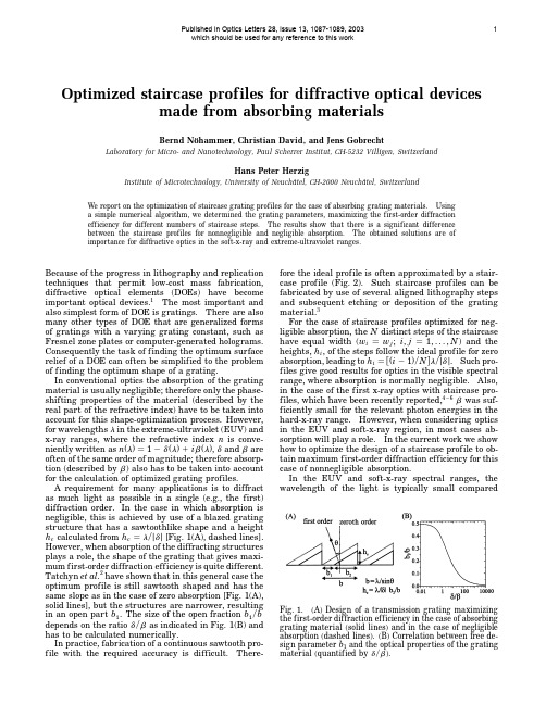
Optimized staircase profiles for diffractive optical devices made from absorbing materialsBernd Nöhammer,Christian David,and Jens GobrechtLaboratory for Micro-and Nanotechnology,Paul Scherrer Institut,CH-5232Villigen,SwitzerlandHans Peter HerzigInstitute of Microtechnology,University of Neuchâtel,CH-2000Neuchâtel,Switzerland We report on the optimization of staircase grating profiles for the case of absorbing grating inga simple numerical algorithm,we determined the grating parameters,maximizing the first-order diffractionefficiency for different numbers of staircase steps.The results show that there is a significant differencebetween the staircase profiles for nonnegligible and negligible absorption.The obtained solutions are ofimportance for diffractive optics in the soft-x-ray and extreme-ultraviolet ranges.Because of the progress in lithography and replicationtechniques that permit low-cost mass fabrication, diffractive optical elements(DOEs)have becomeimportant optical devices.1The most important andalso simplest form of DOE is gratings.There are also many other types of DOE that are generalized formsof gratings with a varying grating constant,such asFresnel zone plates or computer-generated holograms. Consequently the task of finding the optimum surfacerelief of a DOE can often be simplified to the problemof finding the optimum shape of a grating.In conventional optics the absorption of the gratingmaterial is usually negligible;therefore only the phase-shifting properties of the material(described by the real part of the refractive index)have to be taken intoaccount for this shape-optimization process.However,for wavelengths l in the extreme-ultraviolet(EUV)and x-ray ranges,where the refractive index n is conve-niently written as n͑l͒෇12d͑l͒1i b͑l͒,d and b areoften of the same order of magnitude;therefore absorp-tion(described by b)also has to be taken into accountfor the calculation of optimized grating profiles.A requirement for many applications is to diffract as much light as possible in a single(e.g.,the first)diffraction order.In the case in which absorption isnegligible,this is achieved by use of a blazed grating structure that has a sawtoothlike shape and a heighth c calculated from h c෇l͞j d j[Fig.1(A),dashed lines]. However,when absorption of the diffracting structures plays a role,the shape of the grating that gives maxi-mum first-order diffraction efficiency is quite different.Tatchyn et al.2have shown that in this general case the optimum profile is still sawtooth shaped and has the same slope as in the case of zero absorption[Fig.1(A), solid lines],but the structures are narrower,resulting in an open part b1.The size of the open fraction b1͞b depends on the ratio d͞b as indicated in Fig.1(B)and has to be calculated numerically.In practice,fabrication of a continuous sawtooth pro-file with the required accuracy is difficult.There-fore the ideal profile is often approximated by a stair-case profile(Fig.2).Such staircase profiles can be fabricated by use of several aligned lithography stepsand subsequent etching or deposition of the gratingmaterial.3For the case of staircase profiles optimized for neg-ligible absorption,the N distinct steps of the staircasehave equal width(w i෇w j;i,j෇1,...,N)and the heights,h i,of the steps follow the ideal profile for zeroabsorption,leading to h i෇͓͑i21͒͞N͔l͞j d j.Such pro-files give good results for optics in the visible spectral range,where absorption is normally negligible.Also, in the case of the first x-ray optics with staircase pro-files,which have been recently reported,4–6b was suf-ficiently small for the relevant photon energies in the hard-x-ray range.However,when considering optics in the EUV and soft-x-ray region,in most cases ab-sorption will play a role.In the current work we show how to optimize the design of a staircase profile to ob-tain maximum first-order diffraction efficiency for this case of nonnegligible absorption.In the EUV and soft-x-ray spectral ranges,thewavelength of the light is typically smallcomparedFig.1.(A)Design of a transmission grating maximizing the first-order diffraction efficiency in the case of absorbing grating material(solid lines)and in the case of negligible absorption(dashed lines).(B)Correlation between free de-sign parameter b1and the optical properties of the grating material(quantif ied by d͞b).Published in Optics Letters 28, issue 13, 1087-1089, 2003which should be used for any reference to this work1Fig.2.General form of a staircase profile enabling the optimization of the first-order diffraction efficiency.with the period b and the height of the gratings used;therefore in most cases a grating can be treated as a thin structure,and the thin-element approximation can be used (for a discussion of the validity of the thin-element approximation see,for example,Ref.1).In addition,d and b are typically very small;conse-quently ref lections at surfaces between different materials are negligible.With these approximations the diffraction efficiency h can be calculated with the aid of a Fourier analysis of the transmission function.For a discrete profile we get 1h ෇ÉNX i ෇1f i É2,(1)wheref i ෇exp ͑22p h i b ͞d ͒exp ͓2p i ͑h i 2x i ͔͒sin ͑p w i ͒͞p ,(2)and the normalized heights (h i ),widths (w i )andmiddle positions (x i )of the steps are denotedh i ෇h i j d j ͞l ,w i ෇w i ͞b ,x i ෇x i ͞b .(3)Equation (1)is a sum of contributions from each step of the staircase profile shown in Fig.2.The first term in Eq.(2)describes the absorption within one step.The second term gives the phase of each contribution,originating from the material phase shift (h i )and the position of the step within the grating (x i ).The third term is obtained from the Fourier transform of a rect-angular function with width w i .The analytical treat-ment of the problem would be rather complex since the efficiency is a complicated sum over functions of all staircase parameters.Therefore we used a numerical approach,applying a local search algorithm 7to find the optimum values for the parameters in Eq.(3)with respect to diffraction efficiency.The principle of the algorithm is to make small,ran-dom,trial changes in the actual profile,where the change is allowed to take place only if the new profile (the new set of parameters h i ,w i ,and x i )has a higher diffraction efficiency than the previous one.By re-peating this step until a large number (n trial .100)of subsequent trial changes fails to improve the diffrac-tion efficiency,an optimum set of values of h i ,w i ,and x i will ultimately be reached.This kind of algorithm could fail because of the presence of local maxima and as a consequence would never yield reasonable results for the design parame-ters of the grating.However,the numerical resultsshow that the total number of maxima is rather small;therefore it is sufficient to repeat the whole algorithm a few (typically 20)times with different,randomly chosen starting parameters for the grating in order to obtain a parameter set that represents the global optimum with respect to diffraction efficiency.Figure 3shows the numerical results of using this algorithm in the case of a staircase profile with four levels.For low values of absorption (high values of d ͞b )we obtain the expected staircase profile,which has steps with equal width and normalized heights of 0,1͞4,1͞2,and 3͞4.When we go to higher values of absorption,the widths (as well as the heights)of the second and the third steps decrease and finally approach zero.The widths of the first and the fourth steps both increase,and for values of d ͞b near zero they both approach a value equal to half of the grating period b .Therefore in the limit of infinite absorption a conventional binary amplitude grating is obtained.These results for high values of absorption can be qualitatively understood because the staircase profile always has to provide an optimum approximation of the ideal profile in terms of diffraction efficiency.For the ideal grating in the case of strong absorption the main contributions to the diffraction efficiency come from regions of the grating with smallheight.Fig.3.Optimum normalized widths w i (A)and heights h i (B)of a four-step staircase profile as a function of d ͞b of the grating material.Fig.4.First-order diffraction efficiency of a four-step pro-file (solid curve)featuring optimal values for the heights and widths of the steps.In addition,the diffraction ef-ficiency of the ideal continuous profile (see Fig.1)and a four-step profile optimized for negligible absorption aredepicted.Fig.5.First-order diffraction efficiency for different opti-mized grating designs.Therefore it is important to get a good approximation of the region with zero height (provided by the first step with w 1ഠb 1)and a short region with small height at the beginning of the sawtooth (provided by the second and third steps,which therefore tend to have rather small widths and heights in the case of high absorption).In Fig.4the diffraction efficiency of a four-step pro-file with optimal values for h i ,w i ,and x i is depicted.In addition,the diffraction efficiency of the ideal con-tinuous profile and a four-step profile with the con-ventional design rule optimized for zero absorption are plotted for comparison.For high values of d ͞b thetwo different staircase profiles nearly have the same diffraction efficiency,whereas for values of d ͞b below 10a significant difference can be observed.There-fore the optimal design of the staircase profile has to be used in this case to guarantee maximum diffrac-tion efficiency (e.g.,for d ෇2the optimum four-step profile gives 22%diffraction efficiency in comparison with only 16%for a four-step profile optimized for zero absorption).When different step numbers N of the staircase profile are used,similar results are found.For high values of d ͞b (typically d ͞b .10)the anticipated profile optimized for zero absorption [w i ෇w j and h i ෇͑i 21͒͞N ]is obtained.For the case of high absorption the staircase profile gives a good approxi-mation of the ideal continuous profile in regions with small or zero structure height and an inferior approximation in regions of large structure heights,as expected.Figure 5shows the first-order diffraction efficiencies of optimized profiles with different step numbers N .For small values of absorption a larger number N of steps leads to a strongly improved diffraction efficiency,whereas for strong absorption very little difference is found among all profiles.This is because,for all profiles,the normalized width of the region with zero height approaches 1͞2,going to small values of d ͞b .Consequently in the limit of infinite absorption all the staircase profiles will have the same optical properties as a binary amplitude grating.In summary,we have shown that material absorp-tion has to be taken into account for the optimization of gratings in the EUV and x-ray ranges.By use of a numerical local search algorithm we were able to calculate the optimum parameters for maximum first-order diffraction efficiency of gratings with staircase profiles.This work was funded by the Swiss National Sci-ence Foundation. B.N öhammer ’s e-mail address is **********************.References1.H.P.Herzig,ed.,Micro-optics (Taylor &Francis,Lon-don,1998).2.R.Tatchyn,P.L.Csonka,and I.Lindau,J.Opt.Soc.Am.72,1630–1639(1982).3.M.B.Stern,in Micro-optics ,H.P.Herzig,ed.(Taylor &Francis,London,1998),pp.53–86.4.E.Di Fabrizio,F.Romanato,M.Gentili,S.Cabrini,B.Kaulich,J.Susini,and R.Barrett,Nature 401,895–898(1999).5.W.Yun,i,A.A.Krasnoperova,E.Di Fabrizio,Z.Cai,F.Cerrina,Z.Chen,M.Gentili,and E.Gluskin,Rev.Sci.Instrum.70,3537–3541(1999).6.B.N öhammer,J.Hoszowska,H.P.Herzig,and C.David,presented at the X-Ray Microscopy Conference 2002,Grenoble,France,July 29–August 2,2002.7.E.Aarts and J.K.Lenstra,Local Search in Combinato-rial Optimization (Wiley,Chichester,U.K.,1997).。

The ASCA X-ray spectrum of the powerful radio galaxy 3C109

Mon.Not.R.Astron.Soc.000,000–000(1997)The ASCA X-ray spectrum of the powerful radio galaxy3C109S.W.Allen1,A.C.Fabian1,E.Idesawa2,H.Inoue3,T.Kii3,C.Otani41.Institute of Astronomy,Madingley Road,Cambridge CB30HA,2.Department of Physics,University of Tokyo,Hongo,Bunkyo-ku,Tokyo,Japan3.Institute of Space and Astronautical Science,Yoshinodai,Sagamihara,Kanagawa229,Japan4.RIKEN,Institute of Physical and Chemical Research,Hirosawa,Wako,Saitama351-01,Japan10January1997ABSTRACTWe report the results from an ASCA X-ray observation of the powerful Broad LineRadio Galaxy,3C109.The ASCA spectra conﬁrm our earlier ROSAT detection of in-trinsic X-ray absorption associated with the source.The absorbing material obscures acentral engine of quasar-like luminosity.The luminosity is variable,having dropped bya factor of two since the ROSAT observations4years before.The ASCA data also pro-vide evidence for a broad iron emission line from the source,with an intrinsic FWHMof∼120,000km s−1.Interpreting the line asﬂuorescent emission from the inner partsof an accretion disk,we can constrain the inclination of the disk to be>35degree,and the inner radius of the disk to be<70Schwarzschild radii.Our results supportuniﬁed schemes for active galaxies,and demonstrate a remarkable similarity betweenthe X-ray properties of this powerful radio source,and those of lower luminosity,Seyfert1galaxies.Key words:galaxies:active–galaxies:individual:3C109–X-rays:galaxies1INTRODUCTIONUniﬁed models of radio sources propose that radio galaxies and radio-loud quasars are basically the same population of objects,viewed at diﬀerent orientations(Orr&Browne 1982;Scheuer1987;Barthel1989).The nucleus is only di-rectly visible in quasars,the radio axis of which points within ∼45degree of the line of sight.In the case of radio galaxies the axis is closer to the plane of the Sky and the nucleus is obscured from view by material in the host galaxy,possibly in a toroidal distribution.The powerful Broad Line Radio Galaxy(BLRG)3C109 appears to be oriented at an intermediate angle.The nucleus is reddened,E(B−V)∼0.9,and polarized in the optical waveband(Rudy et al.1984;Goodrich&Cohen1992),sug-gesting that our line of sight passes through the edge of the obscuring material.The dereddened luminosity of the nucleus,V=−26.2(Goodrich&Cohen1992)identiﬁes the source as an intrinsically luminous quasar.Obscuration is also seen at X-ray wavelengths(Allen&Fabian1992). 3C109was serendipitously observed with the Position Sen-sitive Proportional Counter(PSPC)on ROSAT in1991Au-gust.The PSPC spectrum exhibits soft X-ray absorption in excess of that expected from material within our own Galaxy,implying an intrinsic equivalent hydrogen column density at the redshift of the source(z=0.3056;Spinrad et al.1985)of∼5×1021atom cm−2.The intrinsic(unab-sorbed)X-ray luminosity of the source(0.1−2.4keV)de-termined from the PSPC data is∼5×1045erg s−1,making it one of the most X-ray luminous objects within z∼0.5; only the QSOs3C273and E1821+643have higher X-ray lu-minosities(and3C273may have a signiﬁcant beamed com-ponent to its X-ray emission).We present here the results of an ASCA X-ray observa-tion of3C109.The ASCA data conﬁrm the results of Allen &Fabian(1992)on excess absorption,and allow us to ex-plore further the X-ray properties of this remarkable source. We show that3C109has decreased in brightness by about a factor of two since the ROSAT observations,to aﬂux level comparable with that observed with the Imaging Propor-tional Counter(IPC)on the Einstein Observatory in1979 (Fabbiano et al1984).Also,of particular interest is the de-tection of a strong,broad iron line in the ASCA spectra. This result implies that most of the X-ray emission from 3C109is unbeamed.Modelling the line asﬂuorescent Fe K emission from an accretion disk,we are able to constrain both the inclination and inner radius of the disk.The X-ray properties of3C109are shown to be remarkably similar to those of many lower-power,Seyfert1galaxies.Throughout this paper we assume a value for the Hubble constant of H0=50km s−1Mpc−1and a cosmological deceleration pa-rameter q0=0.5.22THE ASCA OBSER V ATIONSThe ASCA X-ray astronomy satellite(Tanaka,Inoue& Holt1994)consists of four separate nested-foil telescopes, each with a dedicated X-ray detector.The detectors in-clude two Solid-state Imaging Spectrometers or SISs(Burke et al.1991,Gendreau1995)and two Gas scintillation Imaging Spectrometers or GISs(Kohmura et al.1993). The SIS instruments provide high quantum eﬃciency and good spectral resolution,∆E/E=0.02(E/5.9keV)−0.5.The GIS detectors provide a lower resolution,∆E/E= 0.08(E/5.9keV)−0.5,but cover a larger(∼50arcmin diam-eter)circularﬁeld of view.3C109was observed with ASCA on1995Aug28-29. The SIS observations were made in the standard1-CCD mode(Day et al.1995)with the source positioned at the nominal pointing position for this mode.X-ray event lists were constructed using the standard screening criteria and data reduction techniques discussed by Day et al.(1995). The observations are summarized in Table1.Source spectra were extracted from circular regions of radius4arcmin(SIS0),3.5arcmin(SIS1)and6arcmin (GIS2,GIS3),respectively.For the SIS data,background spectra were extracted from regions of the chip relatively free of source counts.For the GIS data,background spectra were extracted from circular regions,the same size as the source regions,and at similar distance from the optical axes of the telescopes.Spectral analysis was carried out using the XSPEC spectralﬁtting package(Shafer et al.1991).For the SIS data,the1994Nov9version of the SIS response matrices were used.For the GIS data the1995Mar6response ma-trices were used.The spectra were binned to have a mini-mum of20counts per Pulse Height Analysis(PHA)channel, thereby allowingχ2statistics to be used.In general,best-ﬁt parameter values and conﬁdence limits quoted in the text are the results from simultaneousﬁts to all4ASCA data sets,with the normalization of the power-law continuum al-lowed to vary independently for each data set.3RESULTS3.1Conﬁrmation of excess X-ray absorptionin3C109The principal result of the ROSAT PSPC observation of 3C109(Allen&Fabian1992)was the detection of X-ray absorption in excess of the Galactic value determined from 21cm HI observations.The ASCA data allow us to verify and expand upon this result.The ASCA data wereﬁrst examined using a simple ab-sorbed power law model.This allows direct comparison with the results of Allen&Fabian(1992).The free parameters in theﬁts were the column density of the absorbing mate-rial,N H,the photon index of the power law emission,Γ, (both parameters were forced to take the same value in all4 ASCA data sets)and the normalizations,A1,of the power-law emission.(Due to the range of source extraction regions used,and known systematic diﬀerences in theﬂux calibra-tion of the diﬀerent ASCA detectors,the value of A1was allowed to vary independently for each data set).The best ﬁt parameter values and90per cent(∆χ2=2.71)conﬁ-Figure1.(Upper panel)The SIS and GIS spectra of3C109with the bestﬁtting absorbed power-law model(Model A)overlaid. (Lower panel)The residuals to theﬁt in units ofχ.(For plotting purposes the data have been rebinned along the energy axis by a factor7.)Figure2.(Upper panel)The ratio of data to model,where the model is the best-ﬁt Model A,but with the absorption reset to the Galactic value(assumed to be3×1021atom cm−2).Note the large negative residuals at energies below2keV which are due to the excess absorption,and the evidence for a broad,redshifted emission line feature at∼5keV.For plotting purposes,the SIS (open circles)and GIS(ﬁlled squares)data sets have been av-eraged together and binned by a factor of20along the energy axis.The ASCA X-ray spectrum of the powerful radio galaxy 3C1093Table 1.Observation summaryInstrument Observation Date Exposure (ks)ASCA SIS01995Aug 28/2936.0ASCA SIS1””35.0ASCA GIS2””35.0ASCA GIS3””35.0ROSAT PSPC 1991Aug 3022.1Einstein IPC1979Mar 71.86Notes:X-ray observations of 3C109.Exposure times are for the ﬁnal X-ray event lists after standard screening criteria and corrections have beenapplied.Figure 3.Joint conﬁdence contours on the photon index and total column density,determined with spectral Model A (Table 3).Contours mark the regions of 68,90and 99per cent conﬁdence (∆χ2=2.30,4.61and 9.21respectively).dence limits obtained with this simple model are presented in Table 3(Model A).The SIS and GIS spectra with their best-ﬁtting models (Model A)overlaid are plotted in Fig.1.For illustrative purposes,in Fig.2we show the best ﬁt model with the column density reset to the Galactic value (assumed to be 3.0×1021atom cm −2).Note the large negative residuals at energies,E <2keV,which demonstrate the eﬀects of the excess absorption,and the broad positive residual at E ∼5keV,which will be discussed in more detail in Section 3.3.The ASCA results clearly conﬁrm the PSPC result on excess absorption in the X-ray spectrum of 3C109.Assuming that the absorber lies at zero redshift we determine a total column density along the line of sight of 5.30±0.42×1021Figure 4.Joint conﬁdence contours (68,90and 99per cent con-ﬁdence)on the column density and redshift of the excess absorber in 3C109(using spectral Model B).atom cm −2(90per cent conﬁdence limits).This is in goodagreement with the PSPC result of 4.2+1.9−1.6×1021atom cm −2.The ASCA result on the photon index,Γ=1.78+0.05−0.06,is also in excellent agreement with the PSPC result of1.78+0.85−0.76,although is more ﬁrmly constrained.The joint conﬁdence contours on Γand N H are plotted in Fig.3.We have examined the constraints the ASCA spectra can place on the redshift of the excess absorbing mate-rial.The Galactic column density along the line of sight to 3C109,determined from 21cm observations,is 1.46×1021atom cm −2(Jahoda et al.1985;Stark et al.1992),although Johnstone et al.(1992)suggest a slightly higher value of ∼2.0×1021atom cm −2,and Allen &Fabian (1996)in-fer a value of ∼3.0×1021atom cm −2from X-ray stud-ies of the nearby cluster of galaxies Abell 478.Modelling4the ASCA spectra with a two-component absorber,with a Galactic(zero-redshift)column density of3.0×1021atom cm−2,and a component with variable column density and redshift,we obtain the joint conﬁdence contours on the red-shift and column density of the excess absorption plotted in Fig.4.The best-ﬁt parameter values and90per cent conﬁdence limits for the two-component absorption model (Model B)are also summarized in Table3.3.2Variation of the X-ray luminosityTheﬂux measurements for3C109are summarized in Table2.Results are presented for both SIS instruments in the1.0−2.0and2.0−10.0keV(observer frame)energy bands.(The GIS detectors provide less accurateﬂux esti-mates).Also listed in Table2are theﬂuxes observed with the ROSAT PSPC in August1991and the IPC on Einstein Observatory in March1979.We see that in the overlapping 1.0−2.0keV energy band,the brightness of3C109has de-creased by a factor∼2since1991.Theﬂux determination from the ASCA data is now consistent with that inferred from the IPC observation in1979.Also listed in Table2are the intrinsic(absorption-corrected)X-ray luminosities of the source inferred from the observations.(Here the energy bands correspond to the rest-frame of the source).The absorption-corrected2−10keV luminosity inferred from the ASCA spectra is2.1×1045 erg s−1.(We assume that during the Einstein IPC observa-tions the source had the same spectral shape as determined from the ASCA observations.)3C109has also been observed to vary at near-infrared wavelengths.Rudy et al.(1984)found variations of a factor ∼2in the J band over aﬁve year span from1978to1983. Elvis et al.(1984)similarly reported variations in the J,H and K bands of∼50per cent(in the same sense)on a timescale of2–3years between1980and1983.3.3Discovery of a broad iron lineThe residuals to theﬁts with the simple power-law mod-els,presented in Figs.1and2,exhibit an excess of counts in a line-like feature at E∼5.0keV.X-ray observations of Seyfert galaxies(Nandra&Pounds1994and references therein)show that many such sources exhibit a strong emis-sion line at E∼6.40keV(in the rest frame of the object). This is normally attributed toﬂuorescent Fe K emission from cold material irradiated by the nucleus.Weﬁnd that theﬁt to the ASCA data for3C109is sig-niﬁcantly improved by the introduction of a Gaussian line at E∼5keV(∆χ2=9.2for3extraﬁt parameters;an F-test indicates this to be signiﬁcant at the97per cent level.)The best-ﬁt line energy is5.09+0.44−0.38keV(corresponding to6.61+0.57−0.50keV in the rest frame of the source.Note that if aﬁxed rest-energy of6.4keV is assumed,the introduction of the Gaussian component becomes signiﬁcant at the∼99per cent conﬁdence level).The data also indicate that the line isbroad,with a1sigma width of0.65+0.81−0.36keV.The equivalentwidth of the line is300+600−200eV.The width and energy of theline suggest that it is due toﬂuorescence from a rapidly ro-tating accretion disk–as is thought to be the case in lower luminosity Seyfert galaxies(Tanaka et al.1995;Fabianet Figure5.Joint conﬁdence contours(68,and90per cent conﬁ-dence)on the normalization,A2,and inclination,θ,of the disk line using spectral Model D(following Fabian et al.1989).al.1995).The bestﬁtting parameters and conﬁdence limits for the power-law plus Gaussian model(Model C)are sum-marized in Table3.Note that the emission feature is not well-modelled by the introduction of an absorption edge at higher energies[the introduction of an edge into the simple absorbed power-law model(Model A)does not signiﬁcantly improve theﬁt].Note also that the measured lineﬂux is not signiﬁcantly aﬀected by the small systematic bump in the XRT response at E∼5.5keV(which produces a nar-row,positive residual with aﬂux of a few per cent of the continuumﬂux at that energy).3.4Modelling the line as a disklineAlthough the simple Gaussian model provides a reason-able description of the5.0keV emission feature,the ASCA data suggest that the line proﬁle is probably more ing two Gaussian components to model the line proﬁle,we obtain the bestﬁt for a broad component with a rest energy consistent with6.4keV,and a narrow com-ponent with an energy6.8±0.1keV(in the rest-frame of the source).These results are similar to those obtained for nearby,lower-luminosity Seyfert galaxies(e.g.Mushotzky et al1995;Tanaka et al1995;Iwasawa et al.1996)where the line emission is thought to originate from the inner regions of an accretion disk surrounding a central,massive black hole(Fabian et al.1989).We have therefore modelled the broad line in3C109us-ing the Fabian et al.(1989)model for line emission from a relativistic accretion disk.The rest-energy of the line(in the emitted frame)wasﬁxed at6.40keV,the energy appropri-ate for Fe Kﬂuorescence from cold material.(The eﬀects of cosmological redshift were incorporated into the model.) The accretion disk was assumed to extend over radii from3The ASCA X-ray spectrum of the powerful radio galaxy3C1095 Table2.X-rayﬂux of3C109Instrument Date F X L X2-10keV1-2keV2-10keV1-2keV ASCA SIS01995Aug28/2948.5±1.69.50±0.2321.4±0.36.69+0.76−0.71 ASCA SIS1””46.3±2.19.76±0.3221.3±0.37.68+1.10−0.890.1-2.4keV1-2keV0.1-2.4keV1-2keVROSAT PSPC1991Aug3028.9±2.618.2±0.745+147−2512.1+6.3−3.50.5-3.0keV1-2keV0.5-3.0keV1-2keVEinstein IPC1979Mar720±68.3±2.516.5±5.06.2±1.9Notes:The X-rayﬂux and luminosity of3C109measured with ASCA,ROSAT and the Einstein Observatory.Fluxes are in units of10−13erg cm−2s−1and are deﬁned in the rest frame of the observer.Luminosities are in1044erg s−1,are absorption corrected,and are quoted in the rest frame of the source.Errors are90per cent(∆χ2=2.71)conﬁdence limits.to500Schwarzschild radii(hereafter R s)and cover a solid angle of2πsteradians.The emissivity was assumed to follow a standard disk radiation law.Only the disk inclination and line strength were free parameters in theﬁt.The bestﬁt parameters and90per cent conﬁdence limits obtained with the diskline model are listed in Table3(Model D).The in-troduction of the diskline component signiﬁcantly improves theﬁt to the ASCA data with respect to the power-law model(∆χ2=8.9for2extraﬁt parameters,which an F-test indicates to be signiﬁcant at the99per cent conﬁdence level).In Fig.5we show the joint conﬁdence contours on the inclination of the disk,θ,versus the line strength,A2.The 90per cent(∆χ2=2.71)constraint on the inclination is θ>35degree.We have also examined the constraints that may be placed on the inner radius,r in,of the accretion disk with the diskline model.The data were re-ﬁtted with r in included as a free parameter.The preferred value for r in is3R s,with a90per cent conﬁdence upper limit of70R s. (Note that for an ionized disk,with a rest-energy for the line of6.7keV,the inclination is constrained toθ>18degree.) The eﬀects of introducing a further,ﬂatter power-law component into theﬁts,such as may be required to ac-count for reﬂected emission from the illuminated face of an accretion disk,or synchrotron self-Compton emission from within a jet,were also examined.The introduction of aﬂat-ter power-law component does not signiﬁcantly improve the ﬁts.However,the ASCA spectra permit(with no signiﬁcant change inχ2)the inclusion of a continuum spectrum appro-priate for reﬂection from a cold disk,subtending a solid angle of2πsteradians to the primary X-ray source,oriented at any inclination consistent with the results from the disklineﬁts. 4DISCUSSIONThe ASCA results on excess X-ray absorption in3C109con-ﬁrm and reﬁne the earlier ROSAT results(Allen&Fabian 1992).The ASCA data show(under the assumption that all of the absorbing material lies at zero redshift)that theX-ray spectrum of the source is absorbed by a total col-umn density of5.30+0.42−0.42×1021atom cm−2(Model A).This compares to a Galactic column density of∼3.0×1021atom cm−2(Allen&Fabian1996).If we instead assume that the excess absorption,over and above the Galactic value,is due to material at the redshift of3C109,we determine an in-trinsic column density of4.20+0.83−0.78×1021atom cm−2.Note that these results assume solar abundances in the absorbing material(Morrison&McCammon1983).The X-ray absorption measurements are in good agree-ment with optical results on the polarization and intrinsic reddening of the source.Goodrich&Cohen(1992)deter-mine an intrinsic continuum reddening of E(B−V)∼0.9, in addition to an assumed Galactic reddening of E(B−V)= ing the standard(Galactic)relationship between E(B−V)and X-ray column density,N H/E(B−V)= 5.8×1021atom cm−2mag−1(Bohlin,Savage&Drake1978), the total reddening observed,E(B−V)∼1.2,implies a total X-ray column density(Galactic plus intrinsic)of∼7.0×1021 atom cm−2.This result is similar to the X-ray column den-sity inferred from the ASCA spectra using model B and conﬁrms the presence of signiﬁcant intrinsic absorption at the source.Note that this result also suggests that the dust-to-gas ratio in3C109is similar to that in our own Galaxy.Further constraints on the distribution of the absorbing gas are obtained from the optical emission-line data pre-sented by Goodrich&Cohen(1992).In the narrow line re-gion(NLR),the observed Blamer decrement of Hα/Hβ= 5.8implies(for an assumed recombination ratio of3.2)an E(B−V)value∼ing the relationship of Bohlin, Savage&Drake(1978)this implies an X-ray column den-sity to the NLR of∼2.8×1021atom cm−2,in good agree-ment with the Galactic column density of∼3.0×1021atom cm−2determined by Allen&Fabian(1996)and adopted in the X-ray analysis presented here.The Balmer decrement in the broad line region(BLR)is very steep(Hα/Hβ=13.2). Although this value cannot be reliably used to infer the ex-tinction to the BLR,the intrinsic line ratio is unlikely to6Table3.Results of the spectral analysisMODEL PARAMETERSAΓA1N H———χ2/DOFwabs(pow)1.78+0.05−0.061.38+0.10−0.100.530+0.042−0.042———638.9/633BΓA1N H N H(z)——χ2/DOFwabs zwabs(pow)1.77+0.05−0.061.35+0.10−0.090.3000.420+0.083−0.078——641.6/633CΓA1N H EσA2χ2/DOFwabs(pow+gau)1.86+0.12−0.081.47+0.16−0.120.558+0.056−0.0465.09+0.44−0.380.65+0.81−0.362.1+4.3−1.3629.7/630DΓA1N H EθA2χ2/DOFwabs(pow+diskline)1.87+0.08−0.081.48+0.14−0.130.561+0.052−0.0466.4090+0.0−552.4+1.4−1.4630.0/631Notes:A summary of best-ﬁt parameters and90per cent(∆χ2=2.71)conﬁdence limits from the spectral analysis of the ASCA data.Results are shown for four diﬀerent modelsﬁtted simultaneously to the data for all four ASCA detectors.Γis the photon index of the underlying power-law continuum from the source.A1is the normalization of the power law component in the S0detector in10−3photon keV−1cm−2s−1at1keV.N H is the equivalent hydrogen column density in1022atom cm−2at zero redshift.In Model B,N H(z)is the best-ﬁt intrinsic column density at the source for an assumed Galactic column density of0.3×1022atom cm−2.In Model C,E is the energy of the Gaussian emission line in the frame of the observer,σis the one-sigma line width in keV,and A2is the line strength in10−5photon cm−2s−1.In Model D,E is the rest-energy of the line in the emitted frame,θis the inclination of the disk in degree,and A2is again the line strength in10−5photon cm−2s−1.be above5,suggesting a total line-of sight reddening to the BLR of E(B−V)∼>0.8.Thus,the BLR is likely to be intrin-sically reddened by E(B−V)∼>0.3.The optical emission line results are therefore consistent with the two-component absorber model(B),with the column density of the intrinsic absorber being comparable with the Galactic component.3C109is the most powerful object in which a strong broad iron line has been resolved to date.Several more lu-minous quasars observed with ASCA do not show any iron emission or reﬂection features(Nandra et al1995).The next most luminous object with a conﬁrmed broad line is 3C390.3(Eracleous,Halpern&Livio1996)which is about 10times less luminous in both the X-ray and radio bands than3C109.The equivalent widths of the lines in both ob-jects are∼300eV and therefore similar to those observed in lower-luminosity Seyferts.This argues against any X-ray ‘Baldwin eﬀect’(as proposed by Iwasawa&Taniguchi1993).The line emission from3C109is most plausibly due to ﬂuorescence from the innermost regions of an accretion disc around a central black hole(Fabian et al1995).Our results constrain the inner radius of the accretion disk to be<70R s and the inclination of the disk to be>35degree.The strong iron line observed in3C109,and the lack of evidence for a synchrotron self-Compton continuum in the X-ray spectrum, both suggest that little radiation from the jet is beamed into our line of sight.The inclination determined from the ASCA data is larger than the angle proposed by Giovannini et al.(1994) based on the jet/coreﬂux ratio of the source(θ<34de-gree).However,the jet/coreﬂux arguments are based on simple assumptions about the average orientation angles for radio galaxies and neglect environmental eﬀects.The con-ﬂict with the X-ray results may indicate that the situation is more complicated.Giovannini et al.(1994)also present constraints on the inclination from VLBI observations of the jet/counterjet ratio,which requireθ<56degree.The VLBI constraint,together with the ASCA X-ray constraint, then suggests35<θ<56degree.Our results on3C109are in good agreement with the uniﬁcation schemes for radio sources and illustrate the power of X-ray observations for examining such models.The pre-ferred,intermediate inclination angle for the disk in3C109 is in good agreement with the results on X-ray absorption, polarization and optical reddening of the source,all of which suggest that our line of sight to the nucleus passes closes to the edge of the surrounding molecular torus.The results on the broad iron line reveal a striking similarity between the X-ray properties of3C109and those of lower power,Seyfert 1galaxies(Mushotzky et al1995;Tanaka et al1995;Iwa-sawa et al1996).This is despite the fact that the X-ray power of3C109exceeds that of a typical Seyfert galaxy by ∼2orders of magnitude.5ACKNOWLEDGEMENTSWe thank K.Iwasawa,C.Reynolds and R.Johnstone for discussions and the annonymous referee for helpful and con-structive comments concerning the intrinsic reddening in 3C109.SW A and ACF thank the Royal Society for support.The ASCA X-ray spectrum of the powerful radio galaxy3C1097 REFERENCESAllen S.W.&Fabian A.C.,1992,MNRAS,258,29PAllen S.W.&Fabian A.C.,1996,MNRAS,in pressBarthel P.D.,1989,ApJ,336,606Bohlin R.C.,Savage B.D.,Drake J.F.,1978,ApJ,224,132Burke B.E.et al.1991,IEEE Trans.,ED-38,1069Day C.,Arnaud K.,Ebisawa K.,Gotthelf E.,Ingham J.,MukaiK.,White N.,1995,the ABC Guide to ASCA DataReduction,NASA GSFCElvis M.,Willner S.P.,Fabbiano G.,Carleton N.P.,LawrenceA.,Ward M.,1984,ApJ,280,574Eracleous M.,Halpern J.P.,Livio M.,1996,ApJ,459,89Fabian A.C.,Rees M.J.,Stella L.,White N.E.,1989,MNRAS,238,729Fabian A.C.,Nandra K.,Reynolds C.S.,Brandt W.N.,OtaniC.,Tanaka Y.,1995,MNRAS,277,11LFabbiano G.,Miller L.,Trinchieri G.,Longair M.,Elvis M.,1984,ApJ,277,115Gendreau K.et al.,1995,PASJ,47,L5Giovanni G.et al.,1994,ApJ,435,116Goodrich R.W.,Cohen M.H.,1992,ApJ,391,623Iwasawa K.,Taniguchi Y.,1993,ApJ,413,15LIwasawa K.,Fabian A.C.,Mushotzky R.F.,Brandt W.N.,AwakiH.,Kunieda H.,1996,MNRAS,279,837Jahoda K.,McCammon D.,Dickey J.M.,Lockman F.J.,1985,ApJ,290,229Johnstone R.M.,Fabian A.C.,Edge A.C.,Thomas P.A.,1992,MNRAS,255,431Kohmura Y.et al.,1993,Proc.SPIE,2006,78Morrison R.,McCammon D.M.,1983,ApJ,270,119Mushotzky R.F.,Fabian A.C.,Iwasawa K.,Kunieda H.,Matsuoka M.,Nandra K.,Tanaka Y.,1995,MNRAS,272,9LNandra K.,Pounds K.A.,1994,MNRAS,268,405Nandra K.,et al.1995,MNRAS,276,1Orr M.J.L.,Browne I.W.A.,1982,MNRAS,200,1067Rudy R.J.,Schmidt G.D.,Stockman H.S.,Tokunaga,A.T.,1984,ApJ,278,530Scheuer P.A.G.,1987,in Zensus J.A.&Pearson T.E.,ed,Superluminal Radio Sources,Cambridge University Press,CambridgeShafer R.A.,Haberl F.,Arnaud K.A.,Tennant A.F.,1991,XSPEC User’s Guide,.ESA,NoordwijkSpinrad H.,Djorgovski S.,Marr J.,Aguilar L.,1985,PASP,97,932Stark A.A.,Gammie C.F.,Wilson R.W.,Bally J.,Linke R.A.,Heiles C.,Hurwitz M.,1992,ApJS,79,77Tanaka Y.,Inoue H.,Holt S.S.,1994,PASJ,46L,37Tanaka Y.et al.,1995,Nature,275,659。

TI-83 84 Guide for Introductory Statistics说明书

TI-83/84Guide for Introductory Statistics Includes step-by-step instructions,practice exercises,and links to videotutorials.Covers all calculator featuresneeded for AP®Statistics ExamInstructions excerpted fromAdvanced High School Statistics,3rd ed.available for FREE at /ahssLeah DorazioSan Francisco University High School******************May23,2022Copyright©2022OpenIntro,Inc.Third Edition.Updated:May23,2022.This guide is available under a Creative Commons license.Visit for a free PDF,to download the sourceﬁles,or for more information about the license.AP®is a trademark registered and owned by the College Board,which was not involved in the production of, and does not endorse,this product.2ContentsSummarizing data5 Entering data (5)Calculating summary statistics (5)Drawing a box plot (6)What to do if you cannotﬁnd L1or another list (6)Practice exercises (7)Finding area under the normal curve (7)Find a Z-score that corresponds to a percentile (8)Practice exercises (8)Probability10 Computing the binomial coeﬃcient (10)Computing the binomial formula (11)Computing a cumulative binomial probability (11)Practice exercises (11)Inference for categorical data13 1-proportion Z-interval and Z-test (13)Practice exercises (14)2-proportion Z-interval and Z-test (15)Practice exercises (16)Finding area unders the Chi-square curve (17)Chi-square goodness ofﬁt test (17)Chi-square test for two-way tables (18)Practice exercises (19)Inference for numerical data20 1-sample t-test and t-interval (20)Practice exercises (21)1-sample t-test and t-interval with paired data (22)Practice exercises (23)2-sample t-test and t-interval (24)Practice exercises (26)Introduction to linear regression27 Finding a,b,R2,and r for a linear model (27)What to do if r2and r do not show up on a TI-83/84 (28)What to do if a TI-83/84returns:ERR:DIM MISMATCH (28)34CONTENTS Practice exercises (29)t-test and t-interval for the slope of a regression line (30)Summarizing dataEntering dataTI-83/84:ENTERING DATATheﬁrst step in summarizing data or making a graph is to enter the data set into a e STAT,Edit.1.Press STAT.2.Choose1:Edit.3.Enter data into L1or another list.Calculating summary statisticsTI-84:Usestandard1.2.3.4.5.6.7.TI-83:5Calculating the summary statistics will return the following information.It will be neces-sary to hit the down arrow to see all of the summary statistics.¯x Mean n Sample size or#of data points Σx Sum of all the data values minX MinimumΣx2Sum of all the squared data values Q1First quartileSx Sample standard deviation Med Medianσx Population standard deviation maxX MaximumDrawing a box plotTI-83/84:1.2.3.4.5.6.7.What to do if you cannotﬁnd L1or another listTI-83/84:Restore1.2.3.Practice exercisesGUIDED PRACTICE0.1Enter the following10data points into a list on a calculator:5,8,1,19,3,1,11,18,20,5Find the summary statistics and make a box plot of the data.1Finding area under the normal curveTI-84:FINDING AREA UNDER THE NORMAL CURVEUse2ND VARS,normalcdf toﬁnd an area/proportion/probability to the left or right of a Z-score or between two Z-scores.1.Choose2ND VARS(i.e.DISTR).2.Choose2:normalcdf.3.Enter the Z-scores that correspond to the lower(left)and upper(right)bounds.4.Leaveµas0andσas1.5.Down arrow,choose Paste,and hit ENTER.TI-83:Do steps1-2,then enter the lower bound and upper bound separated by a comma,e.g.normalcdf(2,5),and hit ENTER.1The summary statistics should be¯x=9.1,Sx=7.475,Q1=3,etc.The box plot should be as follows.Find a Z-score that corresponds to a percentileTI-84:FIND A Z-SCORE THAT CORRESPONDS TO A PERCENTILEUse2ND VARS,invNorm toﬁnd the Z-score that corresponds to a given percentile.1.Choose2ND VARS(i.e.DISTR).2.Choose3:invNorm.3.Let Area be the percentile as a decimal(the area to the left of desired Z-score).4.Leaveµas0andσas1.5.Down arrow,choose Paste,and hit ENTER.TI-83:Do steps1-2,then enter the percentile as a decimal,e.g.invNorm(.40),then hit ENTER.Practice exercisesGUIDED PRACTICE0.3Find the area under the normal curve to right of Z=2.32normalcdf gives the result without drawing the graph.To draw the graph,do2nd VARS,DRAW, 1:ShadeNorm.However,beware of errors caused by other plots that might interfere with this plot.3Now we want to shade to the right.Therefore our lower bound will be2and the upper bound will be5(or a number bigger than5)to get P(Z>2)=0.023.GUIDED PRACTICE 0.4Find the area under the normal curve between -1.5and 1.5.4GUIDED PRACTICE 0.6Find the Z-score such that 20percent of the area is to the right of that Z-score.5GUIDED PRACTICE 0.8Approximately what percent of these babies weighed greater than 10pounds?74Herewe are given both the lower and the upper bound.Lower bound is -1.5and upper bound is 1.5.The area under the normal curve between -1.5and 1.5=P (−1.5<Z <1.5)=0.866.5If 20%of the area is the right,then 80%of the area is to the left.Letting area be 0.80,we get Z =0.841./1471-2393/8/57Z =10−7.441.33=ing a lower bound of 2and an upper bound of 5,we get P (Z >1.925)=0.027.Approximately 2.7%of the newborns weighed over 10pounds.Probability and probability distributionsComputing the binomial coeﬃcientTI-83/84:Usesame1.2.3.4.5.6.Example:10Computing the binomial formulaTI-84:Useindependent1.2.3.4.5.6.TI-83:binompdf(n,Computing a cumulative binomial probabilityTI-84:Userences1.2.3.4.5.6.TI-83:follows:Practice exercisesGUIDED PRACTICE0.9Find the number of ways of arranging3blue marbles and2red marbles.8 8Here n=5and k=3.Doing5nCr3gives the number of combinations as10.GUIDED PRACTICE0.10There are13marbles in a bag.4are blue and9are red.Randomly draw5marbles with replacement.Find the probability you get exactly3blue marbles.9GUIDED PRACTICE0.11There are13marbles in a bag.4are blue and9are red.Randomly draw5marbles withreplacement.Find the probability you get at most3blue marbles(i.e.less than or equal to3blue marbles).109Here,n=5,p=4/13,and k=3,so set trials=5,p=4/13and x value=3.The probability is0.1396.10Similarly,set trials=5,p=4/13and x value=3.The cumulative probability is0.9662.Inference for categorical data 1-proportion Z-interval and Z-testTI-83/84:13TI-83/84:Use1.2.3.4.5.6.7.8.Practice exercisesGUIDED PRACTICE0.12Using a calculator,evaluate the conﬁdence interval from the example on intelligent life.Recall that we wanted toﬁnd a95%conﬁdence interval for the proportion of U.S.adults who think there is intelligent life on other planets.The sample percent was68%and the sample size was1,033.11GUIDED PRACTICE0.13Using a calculator,ﬁnd the test statistic and p-value for the example on nuclear energy.Recall that we were looking for evidence that more than half of U.S.adults oppose nuclear energy.The sample percent was54%,and the sample size was1019.1211Navigate to1-PropZInt on the calculator.Toﬁnd x,the number of yes responses in the sample,we multiply the sample proportion by the sample size.Here0.68×1033=702.44.We must round this to an integer,so we use x=702.Also,n=1033and C-Level=0.95.The95%conﬁdence interval is(0.651, 0.708).12Navigate to1-PropZTest on the calculator.Let p0=0.5.Toﬁnd x,do0.54×1019=550.26.This needs to be an integer,so round to the closest integer.Here x=550.Also,n=1019.We are looking for evidence that greater than half oppose,so choose>p0.When we do Calculate,we get the test statistic: Z=2.64and the p-value:p=0.006.2-proportion Z-interval and Z-testTI-83/84:TI-83/84:Practice exercisesGUIDED PRACTICE0.14A quality control engineer collects a sample of gears,examining1000gears from eachcompany andﬁnds that879gears pass inspection from the current supplier and958pass inspection from the prospective e a calculator toﬁnd a95%conﬁdence interval for the diﬀerence(current−prospective)in the proportion that would pass inspection.1313Navigate to2-PropZInt on the calculator.Let x1=879,n1=1000,x2=958,and n2=1000.C-Level is.95.This should lead to an interval of(-0.1027,-0.0553),which matches what we found previously.14Navigate to2-PropZTest on the calculator.Correctly going through the calculator steps should lead to a solution with the test statistic z=-2.977and the p-value p=0.00145.These two values match our calculated values from the previous example to within rounding error.The pooled proportion is given as ^p=0.0133.Note:values for x1and x2were given in the table.If,instead,proportions are given,ﬁnd x1 and x2by multiplying the proportions by the sample sizes and rounding the result to an integer.Finding areas under the chi-square curveTI-84:Chi-square goodness ofﬁt testTI-84:Use1.2.3.4.5.6.7.TI-83:manually,L3Chi-square test for two-way tablesTI-83/84:ENTERING DATA INTO A TWO-WAY TABLE1.Hit2ND x−1(i.e.MATRIX).2.Right arrow to EDIT.3.Hit1or ENTER to select matrix A.4.Enter the dimensions by typing#rows,ENTER,#columns,ENTER.5.Enter the data from the two-way table.TI-83/84:CHI-SQUARE TEST OF HOMOGENEITY AND INDEPENDENCE Use STAT,TESTS,χ2-Test.1.First enter two-way table data as described in the previous box.2.Choose STAT.3.Right arrow to TESTS.4.Down arrow and choose C:χ2-Test.5.Down arrow,choose Calculate,and hit ENTER,which returnsχ2chi-square test statisticp p-valuedf degrees of freedomPractice exercisesGUIDED PRACTICE0.16Use a calculator toﬁnd the upper tail area for the the chi-square distribution with5degrees of freedom and aχ2=5.1.1515Use a lower bound of5.1,an upper bound of1000,and d f=5.The upper tail area is0.4038.16Enter the observed counts into L1and the expected counts into L2.the GOF test.Make sure that Observed:is L1and Expected:is L2.Let df:be5.You shouldﬁnd thatχ2=17.36and p-value=0.004.17First create a2×3matrix with the data.Theﬁnal summaries should beχ2=106.4,p-value isp=8.06×10−24≈0,and df=2.Below is the matrix of expected values:Obama Congr.Dem.Congr.Rep.Approve731.59693.45693.96Disapprove726.41688.55689.04Inference for numerical data 1-sample t-test and t-intervalTI-83/84:20TI-83/84:Use1.2.3.4.5.6.Practice exercisesGUIDED PRACTICE0.19The average time for all runners whoﬁnished the Cherry Blossom Run in2006was93.3 minutes.In2017,the average time for100randomly selected participants was97.3,witha standard deviation e a calculator toﬁnd the T-statistic and p-value for the appropriate test to see if the average time for the participants in2017is diﬀerent than it was in2006.18GUIDED PRACTICE0.20Use a calculator toﬁnd a95%conﬁdence interval for the mean mercury content in croakerwhiteﬁsh(Paciﬁc).The sample size was15,and the sample mean and standard deviation were computed as0.287and0.069ppm(parts per million),respectively.1918Navigate to T-Test.Letµ0be93.3.¯x is97.3,S x is17.0,and n=100.Choose=to correspond to H A.We get t=2.353and the p-value p=0.021.The d f=100−1=99.19Navigate to TInterval.We do not have all the data,so choose Stats.Enter¯x and Sx.Note:Sx is the sample standard deviation(0.069),not the SE of the sample mean.Let n=15and C-Level=0.95. This should give the interval(0.249,0.325).The d f=15−1=141-sample t-test and t-interval with paired dataTI-83/84:1-SAMPLE T-TEST WITH PAIRED DATAUse STAT,TESTS,T-Test.1.Choose STAT.2.Right arrow to TESTS.3.Down arrow and choose2:T-Test.4.Choose Data if you have all the data or Stats if you have the mean and standarddeviation.5.Letµ0be the null or hypothesized value ofµdiff.•If you choose Data,let List be L3or the list in which you entered thediﬀerences(don’t forget to enter the diﬀerences!)and let Freq be1.•If you choose Stats,enter the mean,SD,and sample size of the diﬀerences.6.Choose=,<,or>to correspond to H A.7.Choose Calculate and hit ENTER,which returns:t t statisticp p-value¯x the sample mean of the diﬀerencesSx the sample SD of the diﬀerencesn the sample size of the diﬀerencesPractice exercisesGUIDED PRACTICE0.22Use the data in the table above toﬁnd the test statistic and p-value for a test of H0:µdiﬀ=0versus H A:µdiﬀ=0.2120Navigate to TInterval.We do not have all the data,so choose Stats.Enter¯x=3.58and Sx=13.42. Let n=68and C-Level=0.95.This should give the interval(0.332,6.828).The intervals are equivalent when rounded to two decimal places.21Navigate to T-Test.We do not have all the data,so choose Stats.Enterµ0=0,¯x=3.58,Sx= 13.42,n=68,and choose=µ0since the alternative hypothesis is two-sided.This should give the interval t=2.2and p=0.031.2-sample t-test and t-intervalTI-83/84:2-SAMPLE T-TESTUse STAT,TESTS,2-SampTTest.1.Choose STAT.2.Right arrow to TESTS.3.Choose4:2-SampTTest.4.Choose Data if you have all the data or Stats if you have the means and standarddeviations.•If you choose Data,let List1be L1or the list that contains sample1andlet List2be L2or the list that contains sample2(don’t forget to enter thedata!).Let Freq1and Freq2be1.•If you choose Stats,enter the mean,SD,and sample size for sample1andfor sample25.Choose=,<,or>to correspond to H A.6.Let Pooled be NO.7.Choose Calculate and hit ENTER,which returns:t t statistic Sx1SD of sample1p p-value Sx2SD of sample2df degrees of freedom n1size of sample1¯x1mean of sample1n2size of sample2¯x2mean of sample2TI-83/84: Use1.2.3.4.5.6.Practice exercises22Navigate to2-SampTTest.Because we have the summary statistics rather than all of the data,choose Stats.Let¯x1=3.50,Sx1=5.17,n1=9,¯x2=-4.33,Sx2=2.76,and n2=9.We get t=4.01,and the p-value p=8.4×10−4=0.00084.The degrees of freedom for the test is df=12.2.23Navigate to2-SampTInt.Because we have the summary statistics rather than all of the data,choose Stats.Let¯x1=79.41,Sx1=14,n1=30,¯x2=74.1,Sx2=20,and n2=30.The interval is(−3.6,14.2)with d f=51.9.Introduction to linear regression Finding a,b,R2,and r for a linear modelR,AND r FOR A LINEAR MODELTI-84:FINDING a,b,2Use STAT,CALC,LinReg(a+bx).1.Choose STAT.2.Right arrow to CALC.3.Down arrow and choose8:LinReg(a+bx).•Caution:choosing4:LinReg(ax+b)will reverse a and b.4.Let Xlist be L1and Ylist be L2(don’t forget to enter the x and y values in L1and L2before doing this calculation).5.Leave FreqList blank.6.Leave Store RegEQ blank.7.Choose Calculate and hit ENTER,which returns:a a,the y-intercept of the bestﬁt lineb b,the slope of the bestﬁt liner2R2,the explained variancer r,the correlation coeﬃcientTI-83:Do steps1-3,then enter the x list and y list separated by a comma,e.g. LinReg(a+bx)L1,L2,then hit ENTER.27What to do if r2and r do not show up on a TI-83/84WHAT TO DO IF2r AND r DO NOT SHOW UP ON A TI-83/84If r2and r do now show up when doing STAT,CALC,LinReg,the diagnostics must be turned on.This only needs to be once and the diagnostics will remain on.1.Hit2ND0(i.e.CATALOG).2.Scroll down until the arrow points at DiagnosticOn.3.Hit ENTER and ENTER again.The screen should now say:DiagnosticOnDoneWhat to do if a TI-83/84returns:ERR:DIM MIS-MATCHPractice exercisesGUIDED PRACTICE0.25The data set loan50,introduced in Chapter1,contains information on randomly sampledloans oﬀered through the Lending Club.A subset of the data matrix is shown in Figure1. Use a calculator toﬁnd the equation of the least squares regression line for predicting loan amount from total income.24total income loan amount159********260000600037500025000475000600052540002500066700064007288003000Figure1:Sample of data from loan50.24a=11121and b=0.0043,thereforeˆy=11121+0.0043x.t-test and t-interval for the slope of a regression lineTI-83/84:TI-84:。

issi_how_to_choose_the_right_dram

Figure 1. Effects of Differenhis stress may accumulate to the point that a crack appears at the solder joint, causing an electrical discontinuity. Traditional thin small-outline packages (TSOPs) with Alloy42 leadframes can suffer from this problem. The reason for this is the devices likely would be mounted on a PCB with copper traces and landing pads. When the board is heated, the materials made of copper would expand more readily than those made of Alloy42. Some DRAM manufacturers are introducing copper leadframes for TSOPs to address this issue. A copper leadframe expands and contracts proportionally to the copper pads on the PCB, resulting in reduced stress on the solder joint. Additionally, copper leadframes improve package reliability by reducing thermal resistance. Improved thermal resistance results in better heat dissipation from the chip to the leadframe, and therefore less heat-related stress to the chip. Heat stress to the chip is one of the leading causes of a non-mechanical component failure in a long-life application. Lead-Free Product and Whisker Prevention The European environmental legislation known as Restriction of Hazardous Substances (RoHS) has driven the move to leadfree packaging. Without lead, the tin solder that electrically and physically connects components to boards can develop microscopic metal filaments known as whiskers. These whiskers can bridge metal contacts and cause a short circuit. Solutions such as annealed devices with matte tin plating material can be used to minimize the risk of whisker growth. The electronics industry generally accepts an annealed matte tin plating solution. However, the International Electronics Manufacturing Initiative (iNEMI) lists NiPdAu as the preferred plating material, citing the further reduced risk for whiskers. Some DRAM suppliers use this type of plating for their copper leadframes, targeting systems with no tolerance for whisker potential. While the overall trend is toward lead-free products, some demand for leaded products still exists. This request for leaded support is mostly for ball grid array (BGA) packages. The reason some companies still request leaded product is because they are reviewing statistical reports to ensure the long-term reliability of lead-free products. Thus, in some cases, markets such as networking/telecommunications and automotive, which have long-term product requirements, still require leaded support. Some companies have committed to supporting leaded BGA packages and TSOPs for the next few years.

Anti-Ubiquitin antibody [Ubi-1] Product Informatio

Product nameAnti-Ubiquitin antibody [Ubi-1]DescriptionMouse monoclonal [Ubi-1] to Ubiquitin Host speciesMouse Tested applicationsSuitable for: IHC-P, WB Unsuitable for: IP Species reactivityReacts with: Mouse, Human ImmunogenFull length protein corresponding to Cow Ubiquitin conjugated to keyhole limpet haemocyanin (Glutaraldehyde).Positive controlH9C2 cells IHC-P:FFPE mouse brain alzheimer General notes This product was changed from ascites to tissue culture supernatant on 17 May 2016. Thefollowing lots are from ascites and are still in stock as of 17 May 2016: GR159581-2,GR159581-12, GR159581-13. Lot numbers higher than GR159581-13 will be from tissue culturesupernatant. Please note that the dilutions may need to be adjusted accordingly.The Life Science industry has been in the grips of a reproducibility crisis for a number of years.Abcam is leading the way in addressing this with our range of recombinant monoclonal antibodiesand knockout edited cell lines for gold-standard validation. Please check that this product meetsyour needs before purchasing.If you have any questions, special requirements or concerns, please send us an inquiry and/orcontact our Support team ahead of purchase. Recommended alternatives for this product can befound below, along with publications, customer reviews and Q&AsFormLiquid Storage instructionsShipped at 4°C. Store at +4°C short term (1-2 weeks). Upon delivery aliquot. Store at -20°C long term. Avoid freeze / thaw cycle.Storage bufferPreservative: 0.1% Sodium azide PurityAffinity purified ClonalityMonoclonal Clone number Ubi-1Product datasheetAnti-Ubiquitin antibody [Ubi-1] ab72546 Abreviews 86 References 5 ImagesOverviewPropertiesth thIsotype IgG1Light chain type kappaThe Abpromise guarantee Application notes Is unsuitable for IP.Relevance Function: Ubiquitin exists either covalently attached to another protein, or free (unanchored). Whencovalently bound, it is conjugated to target proteins via an isopeptide bond either as a monomer(monoubiquitin), a polymer linked via different Lys residues of the ubiquitin (polyubiquitin chains)or a linear polymer linked via the initiator Met of the ubiquitin (linear polyubiquitin chains).Polyubiquitin chains, when attached to a target protein, have different functions depending on theLys residue of the ubiquitin that is linked: Lys-6-linked may be involved in DNA repair; Lys-11-linked is involved in ERAD (endoplasmic reticulum-associated degradation) and in cell-cycleregulation; Lys-29-linked is involved in lysosomal degradation; Lys-33-linked is involved in kinasemodification; Lys-48-linked is involved in protein degradation via the proteasome; Lys-63-linkedis involved in endocytosis, DNA-damage responses as well as in signaling processes leading toactivation of the transcription factor NF-kappa-B. Linear polymer chains formed via attachment bythe initiator Met lead to cell signaling. Ubiquitin is usually conjugated to Lys residues of targetproteins, however, in rare cases, conjugation to Cys or Ser residues has been observed. Whenpolyubiquitin is free (unanchored-polyubiquitin), it also has distinct roles, such as in activation ofprotein kinases, and in signaling. Similarity: Belongs to the ubiquitin family. Contains 3 ubiquitin-like domains.Cellular localizationCell Membrane, Cytoplasmic and Nuclear ApplicationsOur Abpromise guarantee covers the use of ab7254 in the following tested applications.The application notes include recommended starting dilutions; optimal dilutions/concentrations should be determined by the end user.TargetImagesImmunohistochemistry (Formalin/PFA-fixed paraffin-embedded sections) - Anti-Ubiquitin antibody [Ubi-1] (ab7254)Image from Ohmi K et al., Plos One.2011;6(11):e27461. Fig 7.; doi:10.1371/journal.pone.0027461 Reproduced under the Creative Commons license/licenses/by/4.0/Immunohistochemical staining of ubiquitin in a 7 months-old MPS IIIA mouse brain (PFA fixed) using ab7254.Sections, 40 µm thick, were cut sagittally on a vibratome. Slices were permeabilized in 1% triton X-100/PBS for 1 hour at room temperature. The samples were placed on vectabond-coated glass slides and dried overnight. They were then rehydrated in PBS and washed in ice-cold methanol for 10 min.The slices were washed in 0.3% H2O2 in methanol at room temperature and incubated sequentially with 0.5% normal donkey serum, ab7254 and biotin-labeled F(ab')2 donkey secondary antibody in Tris-buffered saline (pH 7.5) containing 2% BSA and 0.02% Tween 20. The signal was detected with an ABC kit, visualized with diaminobenzidine and counterstained with hematoxylin.Western blot - Anti-Ubiquitin antibody [Ubi-1] (ab7254)All lanes : Anti-Ubiquitin antibody [Ubi-1] (ab7254) at 1/100 dilutionLane 1 : HeLa cell lysateLane 2 : HeLa cell lysate with MG132Lane 3 : Mouse brain tissue lysateLysates/proteins at 20 µg per lane.SecondaryAll lanes : Anti mouse IgG at 1/10000 dilutionImmunohistochemistry (Formalin/PFA-fixed paraffin-embedded sections) - Anti-Ubiquitin antibody [Ubi-1] (ab7254)IHC image of ab7254 staining in mouse alzheimer brain formalin fixed paraffin embedded tissue section, using MOM detection kit, ab127055. The section was pre-treated using pressure cooker heat mediated antigen retrieval with sodium citrate buffer (pH6) for30mins. The section was incubated with ab7254, 5µg/ml, for 15 mins at room temperature. DAB was used as the chromogen (ab103723). The section was counterstained with haematoxylin and mounted with DPX.For other IHC staining systems (automated and non-automated) customers should optimize variable parameters such as antigen retrieval conditions, primary antibody concentration and antibody incubation times.Immunohistochemistry (Formalin/PFA-fixed paraffin-embedded sections) - Anti-Ubiquitin antibody [Ubi-1] (ab7254)Human normal placenta (ab29745). Staining is localised in the cytoplasm and in the nuclei. Left panel: with primary antibody at 1 ug/ml. Right panel: isotype control. Sections were stained using an automated system DAKO Autostainer Plus, at room temperature: sections were rehydrated and antigen retrieved with the Dako 3 in 1 AR buffers citrate pH6.1 in a DAKO PT Link. Slides were peroxidase blocked in 3% H2O2 in methanol for 10 mins. They were then blocked with Dako Protein block for 10 minutes (containing casein 0.25% in PBS) then incubated with primary antibody for 20 min and detected with Dako envision flex amplification kit for mouse for 30 minutes. Colorimetric detection was completed with Diaminobenzidine for 5 minutes. Slides were counterstained with Haematoxylin and coverslipped under DePeX. Please note that for manual staining we recommend to optimize the primary antibody concentration and incubation time (overnight incubation), and amplification may be required.Western blot - Anti-Ubiquitin antibody [Ubi-1] (ab7254)Image courtesy of an anonymous A breview.HeLa cells were co-transfected with a plasmid expressing a target protein together with Ubi expressing vector for 24 hours and either left untreated (Contr) or were treated with 10 µM MG-132 for 6 hours (+MG132). Then the protein of interest was pulled down using Flag agarose beads and and probed with ab7254 at a 1/2000 dilution. The secondary used was an Alexa-Fluor 680 conjugated goat anti-mouse polyclonal used at a 1/10000 dilution. The protein is known to be degraded through proteasome.Please note: A ll products are "FOR RESEA RCH USE ONLY. NOT FOR USE IN DIA GNOSTIC PROCEDURES"Our Abpromise to you: Quality guaranteed and expert technical supportReplacement or refund for products not performing as stated on the datasheetValid for 12 months from date of deliveryResponse to your inquiry within 24 hoursWe provide support in Chinese, English, French, German, Japanese and SpanishExtensive multi-media technical resources to help youWe investigate all quality concerns to ensure our products perform to the highest standardsIf the product does not perform as described on this datasheet, we will offer a refund or replacement. For full details of the Abpromise, please visit https:///abpromise or contact our technical team.Terms and conditionsGuarantee only valid for products bought direct from Abcam or one of our authorized distributors。

c9015

c9015C9015: A Comprehensive Analysis of Its Features and BenefitsIntroduction:The C9015 is a cutting-edge technological innovation that has revolutionized various industries. It offers a range of advanced features and benefits that enhance productivity, efficiency, and overall performance. In this document, we will delve into the details of the C9015, exploring its key features, advantages, and potential applications.1. Overview of the C9015:The C9015 is a multifunctional device that combines several advanced technologies to deliver exceptional results. It is designed to meet the diverse needs of modern businesses and organizations across industries. Some of its key features include:1.1 Versatility:One of the most prominent features of the C9015 is its versatility. It offers a wide range of functions such as printing, scanning, copying, and optional faxing. This multifunctionalityeliminates the need for multiple devices, thereby optimizing space utilization and reducing operating costs.1.2 Speed and Performance:The C9015 boasts impressive speed and performance, enabling high-quality output in minimal time. With its fast processing capabilities, it can handle large print volumes effortlessly. This ensures smooth workflows and improved productivity in demanding work environments.1.3 User-Friendly Interface:The C9015 is equipped with an intuitive user interface, making it accessible to users of all skill levels. Its touchscreen display simplifies navigation and streamlines operations. Additionally, it supports connectivity with mobile devices, enabling wireless printing and scanning.2. Advantages of the C9015:The C9015 offers numerous advantages that set it apart from traditional devices. Let's explore some of the notable benefits:2.1 Cost Savings:By integrating multiple functions into a single device, theC9015 eliminates the need for separate machines. This results in substantial cost savings for businesses, as they no longer have to invest in individual printers, scanners, copiers, and fax machines. Furthermore, the device operates efficiently, reducing energy consumption and lowering utility bills.2.2 Enhanced Efficiency:With its high-speed performance and streamlined operations, the C9015 significantly improves efficiency in any work environment. Automatic document feeding and duplex printing capabilities further optimize productivity. The device also supports advanced features like cloud printing and wireless scanning, enabling seamless collaboration and remote file access.2.3 Sustainable Solution:The C9015 is designed with sustainability in mind. It incorporates environmentally friendly features such as energy-saving modes and the use of recycled materials. This not only reduces the device's carbon footprint but also aligns with the growing demand for eco-friendly solutions.3. Potential Applications:The C9015 finds extensive applications across various industries. Some potential use cases include:3.1 Offices and Corporations:The C9015 is ideally suited for offices and corporations of all sizes. Its speed, versatility, and user-friendly interface make it the perfect choice for handling a range of tasks, from everyday document printing to complex scanning and archival processes.3.2 Educational Institutions:In educational institutions, the C9015 facilitates efficient printing of course materials, worksheets, and assignments. Its versatility allows teachers and students to easily scan and copy documents, enhancing the learning experience.3.3 Healthcare Facilities:The C9015 provides healthcare facilities with the ability to print and scan medical records, prescriptions, and patient forms securely. The device's high-speed performance ensures quick access to critical information, improving patient care and operational efficiency.Conclusion:The C9015 is a versatile, high-performance device that offers numerous advantages for businesses and organizations. Its combination of cutting-edge features, cost savings, enhanced efficiency, and sustainable design make it an indispensable tool in today's fast-paced world. Whether it's in an office, educational institution, or healthcare facility, the C9015 proves to be a reliable and versatile solution. Embrace the power of the C9015 and take your productivity to new heights.。

Technical Guide for Non-Radioactive Nucleic Acid Labeling & Detection_KPL

Technical Guide for Non-Radioactive Nucleic Acid Labeling and Detectionw w w.k p l.c o mTable of Contents Page Chapter 1 – Overview of Non-Radioactive Labeling and Detection3Chapter 2 – Nucleic Acid Probe Labeling 9Chapter 3 – Southern Blotting 23 Chapter 4 – Northern Blotting 33 Chapter 5 – In-Situ Hybridization41 Chapter 6 – Troubleshooting Guide55 Chapter 7 – Appendix65 Miscellaneous Applications65Buffer Recipes68Related Products69 1800-638-3167 • KPL, Inc. • 301-948-77553800-638-3167 • KPL, Inc. • 301-948-7755Non-rad vs. 32PA variety of methods have been developed to detect specific nucleic acid sequences immobilized on membranes (i.e., dot/slot blot, Southern blot,Northern blot, South-Western blot, colony and plaque lifts) and localized in situ in cells and tissues. 32P has traditionally been used due to the intensity of signal it produces and, thus its ability to facilitate the detection of small amounts of biomolecules on blots. However, 32P is not without its shortcomings. These include issues associated with handling and disposing of hazardous material, long exposure times and short half-life, limiting the stability of probes.In recent years, non-radioactive nucleic acid labeling and detection method-ologies have become available in response to a desire by researchers and their institutions to move away from the use of radioisotopes. Advancements made in the areas of chemiluminescence and fluorescence have allowed for an easier transition. In non-radioactive assays, signal is generated through an enzymaticreaction with a chemiluminescent or chromogenic substrate; alternatively ,detection can occur through the appropriate excitation and emission of a fluorophore-labeled probe. For those laboratories seeking replacement technology to 32P without significant investment in instrumentation, chemiluminescent detection enables equivalent results, easily and quickly captured on digital imaging systems or X-ray film shortly after exposure. It is now possible to detect femtogram quantities of nucleic acid in as little as 10 minutes when a hapten and reporter molecule are used in conjunction with a chemiluminescent substrate. The hazards and regulatory issues surrounding 32P-based detection are no longer a trade-off for sensitive, reproducible results.Optimal non-isotopic nucleic acid detection depends primarily on three variables: 1) the molecule or compound used to label the probe,2) hybridization conditions, and 3) the detection method.Figure 1: Comparison of Southern Blot Detection using Detector Labeling and Detection vs. 32P . Detection of single copy gene, n-myc, from 5 µg of human genomic DNA. Panel 1A: Blot detected with a biotinylated n-myc probe and Detector AP Chemiluminescent Blotting Kit in a 10 minute film exposure. Panel 1B: Detection of the same gene with 32P-labeled probe, 16 hour exposure.Figure 2: Comparison of Southern Blot Detection using Detector Labeling and Detection vs. 32P . HeLa cell total RNA detected using an in vitro transcribed biotinylated ß-actin RNA probe and the Detector AP Chemiluminescent Blotting Kit in a 10 minute film exposure (2A) and a 32P-labeled probe in a 3.5 hour film exposure (2B).Component Effect ActionSodium ion concentration Favors formation of hydrogen bonds Increasing [Na+] increases Tm.Detergent (SDS, Sarkosyl, Tween)Prevents nonspecific ionic interactions Insufficient detergent may result in background.of probe with the membrane.Excessive detergent may reduce sensitivity.Nonspecific nucleic acid Blocks nonspecific hybridization of nucleic Addition of nonspecific nucleic acid can decrease(herring or salmon sperm DNA)acid probe.nonspecific background by binding to non-specific regionson the membrane. Also, if the probe is a whole genomic probe,the herring sperm will block repetitive elements.Excessive amounts of nonspecific nucleic acid willreduce sensitivity.Formamide (deionized)Lowers the Tm of the nucleic acid hybridization.Formamide concentration up to 50% decreases the Tm ofthe nucleic acid hybridization and reduces the optimumhybridization temperatures.Protein solution (Blotto, Denhardt’s)Blocks nonspecific binding of probe to May reduce or increase background depending on thethe membrane.membrane used.Polymer accelerant Increases probe concentration by lowering May reduce or increase background depending on the (PEG, Dextran sulfate, PVP)the active water content.membrane used.Tm = melting temperatureTable 1: Hybridization Solution Components and EffectsThe stability of the nucleic acid duplexes and the stringency of hybridizationconditions determine the efficiency of hybridization. Several factorsdestabilize these hybrids by lowering their melting temperature. Thesefactors can be adjusted to favor formation of specific hybrids with minimalinterference from less specific hybrids. In any assay system, increasingstringency improves specificity with a corresponding loss in sensitivity;conditions should be optimized for specific applications. Table 1 describestypical hybridization solution components and their effects on hybridizationefficiency.The hybridization solution contained in Detector kits was formulated toinclude formamide. As a destabilizer formamide lowers the meltingtemperature of hybrids, increasing the stringency of the probe to targetbinding. Use of this agent results in minimal nonspecific hybridization;less optimization of washes is required by the end user. Unlike aqueoushybridization solutions, buffers containing formamide effectively minimizebackground to allow subsequent detection of single copy genes and lowexpressed transcripts. (Figure 5) Thus, these types of solutions can be appliedmore universally. Blotting procedures may also be expedited through the useof Formamide Hybridization Buffer, reducing an overnight hybridization to2 hours without impact on signal:noise ratio. Note that this is acceptablewhen detecting plasmid DNA or moderately expressed transcripts;however,overnight incubations are required for greatest sensitivity when detectinglow copy genomic DNA and rare mRNA.Detection MethodsDetection can be mediated either directly when using fluorescent haptensor indirectly with the use of binding proteins like antibodies or avidin/streptavidin as in the Detector system. The specific antibody or bindingprotein is coupled to an enzyme or fluorochrome and subsequently visualized Figure 5: Detection of a Low Expressed Transcript with Varying Hybridization Conditions.Duplicate lanes of 5 µg of total RNA from WEHI-231 untreated and anti-IgM treatedcells were electrophoresed on a 1% formaldehyde gel and transferred by a 2 houralkaline method to Biodyne B Nylon Membrane. The membrane was cut in half andhybridized with a biotinylated c-myc riboprobe in either formamide or aqueoushybridization buffer. Detection was carried out using the Detector AP ChemiluminescentBlotting Kit. 5A: When using a formamide-based solution, the c-myc gene was observedas a single band in the control sample (1) and the down-regulated treated sample (2).5B: Significant non-specific binding of the probe to the total RNA resulted on the blothybridized in an aqueous hybridization solution.5800-638-3167 • KPL, Inc. • 301-948-77557800-638-3167 • KPL, Inc. • 301-948-7755Detector Labeling KitsCatalog NumberKit SizeLabeling MethodSensitivityApplicationsRandom Primer DNA 60-01-0030 reactionsOnly 100 ng Biotinylation Kitpurified template needed per reaction.PCR DNA60-01-0130 reactionsAs little as 1 ng Biotinylation Kitgenomic template DNA can be amplified and labeled.RNA in vitro 60-01-0220 reactionsOne reactionTranscription generates enough Biotinylation Kitprobe to hybridize 48-96 blots.Detector Detection KitsCatalog NumberKit SizeDetection MethodSensitivityApplicationsAP Chemiluminescent 54-30-012000 cm 2AP-SA and CDP-StarBlotting Kit54-30-02500 cm 2Chemiluminescent SubstrateHRP Chemiluminescent 54-30-002000 cm 2HRP-SA and LumiGLOBlotting KitChemiluminescent SubstrateChromogenic In situ 60-03-0050 samplesHybridization KitTable 4: Choosing KPL Detector KitsExo- fragment of Klenow DNA polymerase extends primers by catalyzing the addition of nucleotidetriphosphate to the nascent probe from a mixture that includes biotin-dCTPSouthern, Northern and dot blotting; colony and plaque hybridization and in situ hybridization.Incorporation of biotin-dCTP via a thermostable DNApolymerase in the polymerase chain reaction.Southern, Northern, dot blotting; colony and plaque hybridization, and in situ hybridization.DNA located downstream of the RNA polymerasepromoter site is copied in a strand – specific manner into a RNA transcript in thepresence of ribonucleotides (biotin-UTP) and either T7 or SP6 RNA polymerase.HRP-SA and TrueBlue peroxi-dase substrate: Orcein and Eosin Y counterstains Southern and Northern blotting; mRNA in situ hybridization.Detection of single copy genes in 5 µg of genomic DNA,low expressed message in 1-5 µg total RNA or ß-actin in just 50 ng of total RNA after a 10-minute film exposure.Northern BlottingGenomic Southern blotting of single copy genes, plasmid DNA, dot blots, and PCR products.Detection of 0.3 pg DNA with a 15-minute film exposure.Southern blotting,bacterial colony and plaque hybridization dot blots.Sensitivityequivalent to FISH.DNA detection in cells, tissues, and metaphase chromosomes.Fluorescent In situ 60-05-0050 samples CY3/DAPI Hybridization KitCY3-SA: DAPI counterstain5-10 times greater fluorescence than FITC/TRITC labeled probes using the same filters.The remainder of The T echnical Guide to Non-Radioactive Labeling and Detection of Nucleic Acids consists of the detailed procedures for performing specific applications employing biotin and Detector kits. The following table (Table 4) summarizes the properties of the Detector product line, assisting in the selection of the appropriate system for your needs.DNA detection in cells,tissues, and metaphase chromosomes.Introduction to KPL’s Detector™Labeling KitsKPL offers three labeling approaches to the generation of biotinylated nucleic acid probes:• Detector Random Primer DNA Biotinylation Kit• Detector PCR DNA Biotinylation Kit• Detector RNA in vitro Transcription Biotinylation KitBoth random primer and PCR-mediated biotin labeling results in the net synthesis of DNA and amplification. Random primed labeling is catalyzed by Klenow polymerase, the large fragment of E. coli DNA polymerase. The Klenow polymerase lacks 5’ 3’ exonuclease activity of the holoenzyme but still contains the 5’ 3’ polymerase as well as the 3’ 5’ exonuclease proof-reading activity. During the polymerization reaction, Klenow polymerase incorporates not only the non-modified deoxynucleotides but also the hapten-modified substrates (e.g., biotin-dCTP), resulting in a DNA probe with high specific activity. PCR-mediated labeling of probes with biotin allows simultaneous amplification and labeling of DNA. Thermostable T aq DNA polymerase drives the PCR reaction, incorporating biotin into the PCR product via modified deoxynucleosite triphosphates. The end product is homogeneously labeled hybridization probes that can detect sub-picogram amounts of target sequences on blots.Probes generated by either random priming or PCR are typically used in Southern blots; they are also suitable for Northern blots. While DNA probes are commonly used in the detection of nucleic acids on membranes, RNA probes are an advantageous alternative and should be considered particularly when the visualization of low expressed genes is desired. In these cases, detection with riboprobes can be approximately 10 times more sensitive than DNA probes. This increase is accounted for by the great affinity of a riboprobe for the complementary sense strand of the mRNA being detected and the resulting higher stability of the RNA:RNA bond after hybridization.1 Additionally, single stranded RNA probes are not subject to the self-annealing that double-stranded DNA probes are, which decreases the availability of the DNA probes to bind to the immobilized target.Single-stranded RNA probes can be generated by in vitro transcription from RNA polymerase promoters such as SP6, T7 or T3. DNA located downstream of the RNA polymerase promoter site is copied in a strand-specific manner into an RNA transcript in the presence of ribonucleotides and the appropriate RNA polymerase. Because of the nature of transcription reactions, many copies of RNA are produced from the template DNA in a short time. Transcripts can be labeled during synthesis by incorporation of biotin during transcription. The incorporation of biotin-UTP by SP6 or T7 polymerase is very efficient, resulting in highly labeled RNA probes.The following protocols describe in detail the process of biotin labeling nucleic acid probes by random priming, PCR labeling and in vitro transcription using KPL’s Detector Biotin Labeling Kits. For additional assistance while using these systems, the labeling section of the Troubleshooting Chapter (Chapter 6) may be referenced.Detector Random Primer DNA Biotinylation Kit (Cat. No. 60-01-00)The Detector Random Primer DNA Biotinylation Kit provides a method for biotinylating DNA probes through incorporation of biotin-dCTP during random-primer extension.2, 3Six base random sequence oligonucleotides serve as primers for replication of the template DNA. The Exo- fragment of Klenow DNA polymerase extends the primers by catalyzing the addition of nucleotide triphosphate, from a mixture that includes biotin-dCTP, to the nascent probe. Large quantities of biotinylated DNA probes can be generated from a small quantity of template DNA. This labeling method results in the net synthesis of DNA. The use of Exo- Klenow polymerase allows for longer labeling reactions without the risk of degradation of the oligonucleotides.The components of this kit are optimized to maximize amplification of template DNA and sensitivity of target detection.4T emplate requirements – Optimal labeling occurs on templates that range from 300-1000 bp. The probe fragments generated vary in length from 100 to1,000 bases, with the average length being approximately 300 base pairs.Probe storage– Stable for at least one year when stored at -20°C. Because biotinylated probes stick to normal microcentrifuge tubes, it is recommended that probes be stored in low retention or siliconized tubes.Probe quantitation– A pre-labeled quantitation standard is included for determining the relative amount of DNA synthesized during the labeling reaction. The concentration of probe to be used in the hybridization buffer must be optimized for greatest sensitivity and minimal background.• Serial dilutions of quantitation standard and newly labeled probe arefixed to positively charged nylon membrane.• The standard and probe are detected using enzyme-labeled streptavidin, and chemiluminescent or chromogenic substrate.• Endpoint sensitivity of the samples is compared to the standard todetermine the amount of probe generated.Materials and EquipmentKit Components Product Code Volume2.5X Random Primer Solution 600-0001700 µL10X dNTP Mixture 600-0002175 µL Klenow DNA Polymerase 600-000335 µL (Exo-fragment)Control Template DNA 600-000425 µL Stop Buffer 600-0005250 µL DEPC Treated Water 50-86-03 1.0 mL Quantitation Standard 600-0007150 µLSufficient reagents are provided to perform 30 labeling reactions when followingthe protocol described below. Kit components are stable for a minimum of 1 year. Reagents must be stored at –20°C and kept on ice during use. Do not store kitsin a frost-free freezer.9800-638-3167 • KPL, Inc. • 301-948-7755Probe Labeling by Random Priming (continued)Steps Critical Points6. Incubate at 37°C for 1 – 4 hours. One hour is sufficient for most applications. For maximum yield of probe,allow the reaction to proceed for 4 hours. Generally, a reaction beginningwith 200-300 ng template DNA generates 5- to 10-fold amplification ofthe template in an hour, and 10- to 50-fold amplification after 4 hours.7. Add 5 µL Stop Buffer and mix.8. Proceed to Probe dilution, dot blotting It is imperative that the probe be quantitated. If too much probe is used inand detection for quantitation.hybridization, background could occur. If too little probe is used, sensitivitymay be reduced.9. Store at –20°C until ready to quantitate and use.See Probe Quantitation on page 18.NOTES ON…Probe Purification:• Following biotinylation, the newly labeled probes may be separated from unincorporated nucleotides by either ethanol precipitation or using KPL’s SpinPure filters (Catalog No. 60-00-53). This is not necessary for use of probes in Southern and Northern blot detection, as unincorporatednucleotides do not significantly increase background. However, if the probes are to be used for in situ hybridization, we do recommend the removal of unincorporated nucleotides. See page 17 for Probe Purification using the SpinPure filters.Detector™PCR DNA Biotinylation Kit Array The Detector™PCR DNA Biotinylation Kit provides a rapid method forbiotinylating DNA probes through incorporation of biotin-N4-dCTP via athermostable DNA polymerase in the polymerase chain reaction*.5-7Biotinylated probes generated using this kit are highly sensitive and allow forthe identification of low copy target sequences. The process of direct labelingduring PCR results in specific labeling and amplification of the sequence ofinterest even from crude DNA samples.The ratio of biotin dCTP to unlabeled dCTP is optimized to produce probeswith maximal biotin incorporation for detection of low copies or rare targetsin mRNA and plasmid or genomic DNA. Amplification and direct labelingfrom small samples of genomic (1 - 100 ng) or plasmid template (10 pg -1 ng) is most easily achieved by first optimizing the conditions for standardPCR before attempting to label the probe during the reaction.Direct detection of a PCR biotin-labeled fragment is also possible. Thebiotinylated PCR product is electrophoresed, transferred to membrane andsubsequently detected without a probe using enzyme-labeled streptavidin.A signal is then generated using the appropriate chromogenic orchemiluminescent substrate as outlined in any of the detection methodsof the Detector Kits. (See Figure 6)* Purchase of this kit does not constitute a license for PCR. A licensed polymerase andlicensed thermal cycler must be used in conjunction with this product. PCR is coveredby patents owned by Hoffman-La Roche, Inc. and F. Hoffman-La Roche, Inc.Detector PCR DNA BiotinylationAt A GlanceOptimize PCR Conditions With Unmodified dNTPsPrepare PCR Reaction MixPerform PCR ~25 cycles, 40 minutesQuantitate ProbeStore at -20°CStepsCritical Points1. Prepare the reaction mix in a sterile PCR tube inThaw the 10X Labeling Mix on the bench or warm it to room temperature in order as it appears below. Place the tube on ice while pipetting.your hand before use. Improperly thawed dNTPs may result in a failure to produce amplification product.Component Volume Final DEPC Treated Water variable add to 50 µl By adjusting the final concentration of the 10X Labeling Mix included in the 10X PCR Buffer 5 µl 1Xkit, probes of up to 1 kb in length may be generated. For probes less than 25 mM MgCl 24 µl 2.0 µM500 base pairs, a final concentration of 200 µM of each nucleotide is suggested 10X Labeling Mix 5 µl 200 µM each (5 µL/50 µL PCR reaction), and for probes greater than 500 base pairs, Primers1 µl0.5 µM each350 µM of each nucleotide is suggested (8.75 µL/50 µL PCR reaction).(if using the control primers)Taq DNA Polymerase variable 1.25 units/ 50 µl rxn Template1 µl1-10 ng(if using genomic DNA or the control 10 pg-1 ng template)plasmid DNATotal Mix50 µl2. Mix the tube by tapping gently and centrifuging briefly.Probe Labeling by PCRNOTES ON…Getting Started• The following protocol was designed specifically for the PCR labeling of the control template included with this kit. PCR reaction conditions should be optimized for each new template/primer set with unmodified nucleotides before use of this kit. Use the following protocol as a guideline only . • Caution should be taken to minimize introduction of contami-nating DNA and/or DNases to the PCR reaction that may result in amplification of non-specific product or no product. Always wear gloves, wash all work areas appropriately prior to beginning.• Allow all reagents to thaw out completely , then vortex briefly and spin down in a microcentrifuge before pipetting. Keep all reagents on ice while in use except for the 10X Labeling Mix. Pipette reagents slowly and carefully to avoid errors.• The buffers contained in and/or recommended for use with this kit are prepared according to the protocols listed at the end of this chapter, beginning page 20. Recipes for miscellaneous solutions can be found in the Appendix.Materials and EquipmentKit ComponentsProduct CodeVolume 10X Ribonucleotide Labeling Mix 600-001360 µL 10X Transcription Buffer 600-001060 µL ß-Actin Template 600-001716 µL RNase Inhibitor 600-001213 µL SP6 RNA Polymerase 600-001520 µL T7 RNA Polymerase 600-001420 µL DNase I600-001620 µL DEPC Treated Water 50-86-03 1.0 mL Quantitation Standard 600-0007150 µL Spin-Pure Filters60-00-535 filtersSufficient reagents are provided to perform 20 labeling reactions following theprotocol provided in this manual. All reagents must be stored at -20°C except for the Spin-Pure Filters that should be stored at room temperature. Do not store kits in a frost-free freezer. Kit components are stable for a minimum of 1 year from date of receipt when stored as instructed.Quantitation of the probe is essential as the concentration of probe used in the hybridization reaction is critical for greatest sensitivity and minimal background on a membrane.• Serial dilutions of quantitation standard and newly labeled probe are fixed to positively charged nylon membrane.• The standard and probe are detected using enzyme-labeled streptavidin, and chemiluminescent or chromogenic substrate.• Endpoint sensitivity of the samples is compared to the standard to determine the relative amount of probe generated.Probe storage – Stable for at least one year when stored at -20°C. Because biotinylated probes stick to normal microcentrifuge tubes, it is recommended that probes be stored in low retention or siliconized tubes.Detector RNA in vitro Transcription BiotinylationAt A GlancePreparation of DNA TemplatePrepare Labeling reaction mixIncubate at 37°C2 hoursAdd DNase IIncubate at 37°C 15 minutesQuantitate ProbeStore at –20°C[or -70°C for long-term storage]NOTES ON…Getting Started• All tubes and pipet tips should be autoclaved or purchased as RNase free prior to working with RNA.• All glassware and equipment used should be RNase free.• Always wear gloves when working with RNA because human skin contains abundant amounts of RNases.Detector RNA in vitro Transcription Biotinylation KitThe Detector ™RNA in vitro Transcription Biotinylation Kit provides a method for synthesizing biotin labeled RNA probes by in vitro transcription through incorporation of biotin UTP . Strand-specific probes may be generated using either the T7 or SP6 RNA polymerase.9The transcript reaction generates full length, single-stranded RNA probes that can be used in a variety of applica-tions, including membrane and in situ hybridization. The incorporation of biotin UTP by SP6 or T7 polymerase is very efficient, resulting in “hot”labeled RNA probes. These non-isotopic biotin labeled RNA probes are stable for at least one year. Single-stranded RNA probes hybridize more effectively to target molecules because they do not self-hybridize as DNA probes do.10RNA probes offer greater sensitivity than DNA probes because RNA-RNA or RNA-DNA hybrids are more stable than DNA-DNA duplexes in hybridization.Direct detection of a biotin-labeled RNA probe is also possible. The biotinylated transcript can be electrophoresed, transferred to a membrane, and subsequently detected without a probe using fluorochrome-labeled streptavidin or enzyme-labeled streptavidin and a chromogenic or chemiluminescent substrate as directed in any of the detection methods of the Detector kits.The components of this kit are optimized to maximize the synthesis of RNA as well as the sensitivity of target detection.T emplate requirements – In order to generate single stranded RNA probes, you must begin with a DNA template with SP6 or T7 promoter sequences upstream from the desired template sequence. T wo methods to prepare these types of templates are recommended and further detailed in the protocol:• Cloning the DNA into a vector with the SP6 and T7 promoter sequences on either side of the cloning site• PCR of the DNA template with the promoter sequences built into the primers.Kit control – A human ß-Actin DNA template is included in this kit to serve a two-fold purpose: 1) to act as a control for the integrity of the kit components, and 2) to generate a control probe for detection of ß-actin on human or mouse Northern blots. Synthesized in a strand-specific manner,an antisense transcript may be generated using T7 RNA polymerase and a sense transcript may be generated using SP6 RNA polymerase. The expected size of either transcript is ~400 bases. If the control probe is to be used in a Northern blot, the anti-sense (T7) probe must be used.Probe quantitation – The second kit control, the Biotinylated Quantitation Standard is used to quantitate the yield of biotin-labeled RNA probe.Probe Labeling by in vitro Transcription(continued)Steps Critical Points3. Mix the tube by flicking gently and centrifuge briefly.4. Place the tube at 37°C for 2 hours.5. Add 1 µL of DNase I, flick the tube gently, and centrifuge briefly.6. Incubate 37°C for 15 minutes.7. Place the tube on ice or store at –20°C until needed for Because of the high concentration of the probe and its susceptibility toquantitation and analysis.RNases, aliquoting of the probe for storage is recommended. For longterm storage, freeze at -70°C.NOTES ON… Probe Purification:• Following biotinylation, the newly labeled probes may be separated from unincorporated nucleotides by either ethanol precipitation or using KPL’s SpinPure filters (Catalog No. 60-00-53). This is not necessary for use of probes in Southern and Northern blot detection, as unincorporated nucleotides do not significantly increase background. However, if the probes are to be used for in situ hybridization, we do recommend the removal of unincorporated nucleotides. See below for Probe Purification using the SpinPure filters.Probe Purification (optional)Steps Critical Points1. Ensure that the sample reservoir is firmly placed into thefiltrate receiver.2. Add 1XTE to the probe to increase the volume. Do not tear the filter with a pipet tip.Pipette 50 - 500 µL of the sample into the sample reservoir.Cap the Spin-Pure filter and place into a microcentrifuge.3. Centrifuge at 5,000 x g for 15 minutes at room temperature.Continue centrifugation until filter is dry (a volume of 500 µLcan usually be concentrated in 20 minutes).4. If removing primers and nucleotides from amplified product,centrifuge at 14,000 x g.5. Recover sample from the filter with DEPC-treated wateror 1X TE by rinsing the surface. Highest yields result fromtwo rinses of 20 µL each.Gel Analysis of TranscriptSteps Critical Points1. Pre-heat the probe to 68°C for 5 minutes.The expected size of the transcript will be somewhat different whencomparing an RNA probe to a DNA marker lane, but an approximate sizeestimate can still be determined.2. Run 2-5 µL of the probe on either a 1X TBE agarose gel or a Biotinylated transcripts run larger than their unbiotinylated counterparts.formaldehyde gel containing 0.5 µg/mL ethidium bromide.Include DNA or RNA markers on the gel for proper size.3. Transfer the remaining aliquot of sample to a siliconized tube See Probe Quantitation on page 18.and store at 2–8ºC until quantitation.。

1、下载文档前请自行甄别文档内容的完整性，平台不提供额外的编辑、内容补充、找答案等附加服务。
2、"仅部分预览"的文档,不可在线预览部分如存在完整性等问题,可反馈申请退款(可完整预览的文档不适用该条件!)。
3、如文档侵犯您的权益，请联系客服反馈,我们会尽快为您处理(人工客服工作时间：9:00-18:30)。

a r X i v :h e p -e x /0304028v 1 22 A p r 2003DIRC for a Higher Luminosity B FactoryThomas Hadig Stanford Linear Accelerator Center,Stanford University,Stanford,CA 94309for the B A B AR -Dirc Collaboration[1]hep-ex/0304028SLAC–PUB–9715October 2002Abstract The Dirc ,a novel type of Cherenkov ring imaging device,is the primary hadronic particle identiﬁcation system for the B A B AR detector at the asymmetric B-factory Pep-II at SLAC.It is based on total internal reﬂection and uses long,rectangular bars made from synthetic fused silica as Cherenkov radiators and light guides.B A B AR began taking data with colliding beams in late spring 1999.This paper describes the challenges for the Dirc in a higher luminosity environment and shows solutions to these challenges.1Introduction The study of CP -violation using hadronic ﬁnal states of the B8-20008524A6Figure1:Schematic of the Dirc fused silica radiator bar and imaging region.In the following,the variableθC is used to designate the Cherenkov angle,φC denotes the azimuthal angle of a Cherenkov photon around the track direction,and n represents the mean index of refraction of fused silica (n=1.473)within the wavelength acceptance of the Dirc(300nm to600nm).The Cherenkov angle is given by the familiar relation cosθC=1/(nβ)withβ=v/c,the velocity of the particle v and the velocity of light c.For particles withβ≈1,some photons will always lie within the total internal reﬂection limit,and will be transported to either one or both ends of the bar,depending on the particle incident angle.To avoid instrumenting both ends of the bar with photon detectors,a mirror is placed at the forward end,perpendicular to the bar axis,to reﬂect incident photons to the backward,instrumented end(see Figure1).Once photons arrive at the instrumented end,most of them emerge into a water-ﬁlled expansion region, called the standoﬀbox.A fused silica wedge at the exit of the bar reﬂects photons at large angles relative to the bar axis.It thereby reduces the size of the required detection surface and recovers those photons that would otherwise be lost due to internal reﬂection at the fused silica/water interface.The photons are detected by an array of densely packed photomultiplier tubes(PMTs)[7,8],each surrounded by reﬂecting light catcher cones[9] to capture light which would otherwise miss the active area of the PMT.The PMTs are placed at a distance of about1.2m from the end of the bars.The expected Cherenkov light pattern at this surface is essentially a conic section,where the cone opening-angle is the Cherenkov production angle modiﬁed by refraction at the exit from the fused silica window.The Dirc bars are arranged in a12-sided polygonal barrel(see Figure2).Because of the beam energy asymmetry(at theΥ(4S),Pep-II collides9GeV electrons on3.1GeV positrons),particles are produced preferentially forward in the laboratory.To minimize interference with other detector systems in the forward region,the Dirc photon detector is placed at the backward end.The bars are placed into12hermetically sealed containers,called bar boxes,made of aluminum-hexcel panels.Dry nitrogen gasﬂows through each box,and is monitored for humidity to ensure that the bar box to water interface remains sealed.Each bar box contains12 bars,for a total of144bars.Within a bar box the12bars are optically isolated by a∼150µm air gap between2Figure2:Exploded view of the Dirc mechanical support structure.The iron magnetic shield is not shown.neighboring bars,enforced by custom shims made from aluminum foil.The bars are17mm thick,35mm wide,and4.9m long.Each bar is assembled from four1.225m pieces that are glued end-to-end;this length is the longest high-quality bar currently obtainable[6,10].The bars are supported at600mm intervals by small nylon buttons for optical isolation from the bar box.Each bar has a fused silica wedge glued to it at the readout end.The wedge,made of the same material as the bar,is91mm long with very nearly the same width(33mm)as the bars and a trapezoidal proﬁle(27mm high at bar end,and 79mm high at the light exit end).The bottom of the wedge(see Figure1)has a slight(∼6mrad)upward slope to minimize the displacement of the downward reﬂected image due to theﬁnite bar thickness.The12wedges in a bar box are glued to a common10mm thick fused silica window which provides the interface and seal to the puriﬁed water in the standoﬀbox.The standoﬀbox(see Figure2)is made of stainless steel,consisting of a cone,cylinder,and12sectors of PMTs.It contains about6000l of puriﬁed water.Water is used toﬁll this region because it is inexpensive and has an average index of refraction(n≈1.346)reasonably close to that of fused silica,thus minimizing the total internal reﬂection at silica-water interface.Furthermore,its chromaticity index is a close match to that of fused silica,eﬀectively eliminating dispersion at the silica-water interface.The iron gusset supports the standoﬀbox. An iron shield,supplemented by a bucking coil,surrounds the standoﬀbox to reduce theﬁeld in the PMT region to below1G[11].The PMTs at the rear of the standoﬀbox lie on an approximately toroidal surface.The distance from the end of the bar to the PMTs is∼1.17m.Each of the12PMT sectors contains896PMTs(ETL model 9125[7,8])with29mm diameter,in a closely packed array inside the water volume.A double o-ring water seal is made between the PMTs and the vessel wall.The PMTs are installed from the inside of the standoﬀbox and connected via a feed-through to a base mounted outside.The hexagonal light catcher cone is mounted in front of the photocathode of each PMT which results in an eﬀective active surface area light collection fraction of about90%.The Dirc occupies80mm of radial space in the central detector volume including supports and construction3Figure3:Display of an e+e−→µ+µ−event reconstructed in B A B AR with two diﬀerent time cuts.On the left, all Dirc PMTs with signals within the±300ns trigger window are shown.On the right,only those PMTs with signals within8ns of the expected Cherenkov photon arrival time are displayed.tolerances with a total of about19%radiation length thickness at normal incidence.The radiator bars cover a solid angle corresponding to about94%of the azimuth and83%of the c.m.polar angle cosine.3Dirc PerformanceThe performance of the Dirc is inﬂuenced by two factors.First,information from the PMTs has to be separated into background and signal.Second,theθC resolution of the signal has to allow for the separation of diﬀerent particle species.Figure3shows a typical di-muon event(e+e−→µ+µ−).In addition to the signals caused by Cherenkov light from the muon tracks,about500background signals can be seen in the600ns readout window centered around the trigger.This background is dominated by low energy photons from the Pep-II machine hitting the standoﬀbox.The time-to-digital converter(TDC)chip[12]used in the Dirc data readout is designed such that a dead time of about5%occurs at an input rate of250kHz.Some care in machine tuning is required to stay under a limit of250kHz per tube.To monitor this rate,one PMT in each sector is read out via a scaler.Figure4shows the maximum scaler rate as a function of the Pep-II luminosity during data taking in2000and2001.In March 2000the accelerator operated at a peak luminosity of1033cm−2s−1.Figure4(a)shows,at a value corresponding to only one third of the design luminosity,the PMT rates reached a level that caused noticeable dead times. Due to thoseﬁndings,lead shielding was installed in the summer of2000around the beam line components near the backward end-cap.Initially,localized shielding was added in the form of lead bricks which were stacked around the beam pipe and in front of a large quadrupole.This shielding signiﬁcantly improved the background situation so that noticeable TDC dead times were reached only at2.5×1033cm−2s−1(Figure4(b)).During40100200010********200s c a l e r r a t e (k H z )luminosity (1033/cm 2s)Figure 4:Maximum scaler rates measured for three diﬀerent accelerator and shielding conﬁgurations in March 2000(a),October 2000(b)and August 2001(c).the shutdown in January 2001,the localized lead brick shielding was replaced by an engineered,homogeneous lead shielding of 5cm to 8cm thickness covering the inside radius of the standoﬀbox and is easily removable to facilitate access to the central detector and beam line components.As is shown in ﬁgure 4(c),the maximum scaler rates at luminosities of 4.2×1033/cm −2s −1are well below the level that would cause TDC ineﬃciencies.During the shutdown following the 2001-2002run,we plan to replace the TDCs with a faster version with deeper buﬀering that is designed to have a deadtime of less than 5%at 2.5MHz input rate,suitable for luminosities of at least 1034cm −2s −1.The Dirc is intrinsically a three-dimensional imaging device.Photons are focused onto the phototube detection surface via a “pinhole”deﬁned by the exit aperture of the bar,so that the photon propagation angles αx and αy can be measured in two-dimensional space,where x (bar width)and y (bar thickness)are the directions transverse to the bar axis.The travel time of the photon down the bar is also related to the photon propagation angle (αz )with respect to the bar axis.Imaging in the Dirc occurs in all three of these dimensions,by recording the time of the PMT signal.As the track position and angles are known from the tracking system,these three αangles can be used to determine the two angles (θC ,φC ).This over-constraint on the angles is particularly useful in dealing with ambiguities and high background rates.The single photon resolution can be calculated from the geometrical,the chromatic and the transport term.The geometrical uncertainty is,for the pinhole optics of the Dirc ,given by the standoﬀbox size,the bar and the PMT size.With 7.2mrad ,it is the single biggest contribution to the single photon resolution.The chromatic uncertainty originates from the fact that the photons are produced with diﬀerent wavelengths and,therefore,have diﬀerent cone opening angles θC .Using the range in photon wavelength accepted by the PMTs,the chromatic eﬀect contributes to the resolution with 5.4mrad .The ﬁnal uncertainty comes from imperfections of the bars and the glue joints.This transport term is approximately 2mrad to 3mrad .Combining the three contributions,a single photon resolution of σθC ,γ=9.5mrad is expected for the Dirc .52000040000−50050∆θC,γ (mrad)e n t r i e s p e r m r a d Figure 5:The diﬀerence between the measured and expected Cherenkov angle for single photons,∆θC,γfor single muons in µ+µ−events.The curve shows the result of a ﬁt of two Gaussians to the data.The width of the narrow Gaussian is 9.6mrad .Figure 5shows the single photon angular resolution obtained from di-muon events.There is a broad background of less than 10%relative height under the peak that originates mostly from track-associated sources,such as δrays,reﬂections oﬀthe glue-fused silica boundaries,and combinatorial background[13].The width of the peak translates to a resolution of about 9.6mrad ,in good agreement with the expected value.The resolution on the track Cherenkov angle is deﬁned by a correlated term and the single photon resolution which scales with the number of photoelectrons:σθC =σθC ,corr ⊕σθC ,γN pe(1)where N pe is the number of photons detected per track.The number of photoelectrons varies between 16for small values of cos θtrack at the center of the barrel and 60at large values of cos θtrack as is shown in Figure 6.This variation is well reproduced by Monte Carlo simulation and can be understood from the geometry of the Dirc .The number of Cherenkov photons varies with the path length of the track in the radiator,it is smallest at perpendicular incidence at the center and increases towards the ends of the bars.In addition,the fraction of photons trapped by total internal reﬂection rises with larger values of cos θtrack .This increase in the number of photons for forward going tracks is a good match to the increase in performance required at larger momentum.With the present alignment,the track Cherenkov angle resolution for di-muon events is shown in Figure 7.The width of the ﬁtted Gaussian distribution is 2.4mrad compared to the design goal of 2.2mrad .The measured time resolution is 1.7ns ,close to the intrinsic 1.5ns transit time spread of the PMTs.This resolution is used to eﬃciently distinguish background from signal photons but is not suﬃcient to improve the Cherenkov angle resolution.Figure 8shows an example of the use of the Dirc for particle identiﬁcation.The Kπinvariant mass spectra are shown with and without the use of the Dirc for kaon identiﬁcation.The peak corresponds to the decay of the D 0particle.The PID performance of the Dirc has been studied with a sample of pions and kaons,selected kinematically using D 0→K −π+decays from inclusive D ∗production.6-1-0.500.51cos(θtrack )<N γ >Figure 6:Number of detected photons versus trackpolar angle for reconstructed tracks in di-muon events compared to Monte Carlo simulation.The mean number of photons in the simulation has been tuned to match the data.1000015000−10010θC, track (measured) − θC (µ) (mrad)T r a c k s Figure 7:Resolution of the reconstructed Cherenkov polar angle per track for di-muon events.The curve shows the result of a Gaussian ﬁt with a resolution of 2.4mrad .750010001500x 1021.75 1.8 1.85 1.9 1.95K π mass (GeV/c 2)e n t r i e s p e r 5 M e V /c 2Without DIRCWith DIRCFigure 8:Invariant K πinclusive mass spectrum with and without the use of the Dirc for kaon identiﬁcation.The mass peak corresponds to the decay of the D 0particle.The π/K separation power of the Dirc was deﬁned as the diﬀerence of the expected Cherenkov angles for pions and kaons,divided by the measured track Cherenkov angle resolution.As shown in Figure 9,the separation between kaons and pions at 3GeV /c is about 4.4σ,within 10%of the design goal.The eﬃciency for correctly identifying a charged kaon that traverses a radiator bar and the probability to wrongly identify a pion as a kaon are also determined from the inclusive D ∗sample and are shown as a function of the track momentum in Figure 10for a particular choice of particle selection criteria.The kaon selection eﬃciency and pion misidentiﬁcation,integrated over the K and πmomentum spectra of the D ∗control sample,are 97.97±0.07%(stat.only)and 1.83±0.06%(stat.only),respectively.A report on the operational experience with the Dirc detector can be found in [14].4Dirc in Higher Luminosity EnvironmentIn a higher luminosity environment,the accelerator-induced background will cause the main challenge.From a set of special runs taken in February 2002,the background rate as a function of the beam currents I HER and I LER in the high and low energy ring,respectively,and the luminosity L can be parameterized asR =13kHzA I LER +10kHz02468102 2.53 3.54momentum (GeV/c)π-K s e p a r a t i o n (s .d .)Figure 9:Dirc π/K separation versus track momentum measured in D 0→K −π+decays selected kinematically from inclusive D ∗production.Momentum (GeV/c )K a o n I D0.250.50.751123Figure 10:Eﬃciency and misidentiﬁcation probability for the selection of charged kaons as a function of track momentum,for a particular choice of particle selection criteria.The data use D 0→K −π+decays selected kinematically from inclusive D ∗production.9the Dirc will be able to reliably work in this environment.At higher luminosities,such as expected after major Pep-II updates or for Super B A B AR,more changes will be necessary.A solution to high background rates is to reduce the size of the standoﬀbox.However,without modiﬁcations to the design,this would lead to an increase in the geometric resolution term and would cause a considerable decrease in the Dirc performance.A modiﬁed design,as shown inﬁgure11,employs smaller sized photodetectors as well as focusing optics eﬀectively removing the bar size uncertainty in the focusing plane.These two enhancements can be balanced so that the size of the standoﬀregion can be reduced while keeping a similar or improved geometrical resolution.In addition,smaller photodetectors with a better transit time spread will improve the timing resolution of the detector.This can be used to further reduce the background by using tighter time cuts and to reduce the chromatic uncertainty.The travel time of a photon is the diﬀerence between the time the particle hits the bar and the arrival time of the photon.It depends on the path length and the group velocity in the transit medium. The group velocity itself depends on the refractive index.Thus,the travel time and path length yield a measure of the wavelength of the photon.Figure12shows a calculation demonstrating that a timing resolution in the order of100ps is needed for a signiﬁcant improvement in the chromatic uncertainty.Reducing the range of wavelength accepted in the detection system will reduce the range of Cherenkov cone opening angles contributing and,thus,reduce the chromatic uncertainty.The drawback of this solution is the loss in the number of photons detected per track causing a reduced suppression of the single photon resolution term.These two eﬀects can be balanced in order to reach the optimal totalθC resolution.With a timing resolution in the order of100ps,the ratio of the track to detector distance over the path length will provide an additional measure of the photon angle.In some regions of phase space,especially at small dip angles,its resolution will be competitive to the angle resolution from the position of the PMT hit.A more detailed discussion can be found in[15].One of the photon detector candidates is theﬂat panel PMT H-8500by Hamamatsu[16].It has8×8square pads on a size of50mm×50mm.This leads to a high area eﬃciency and packaging density.The timing resolution is expected to be in the range of100ps to200ps.The disadvantage of the currently available model10Figure12:Achievable wavelength resolution as a function of photon wavelength assuming100ps and500ps timing resolution.is its low gain in the order of1.6×106.Studies of the timing resolution on an early pre-production version were encouraging.The time was measured at two thresholds for each signal in order to perform a time walk correction.The corrected time distribution[17]is shown inﬁgure13.Aﬁt to a double Gaussian plus a second order polynomial describes the data well.The narrow Gaussian has a width of125ps.This value is not yet corrected for the light pulse width and instrumentational eﬀects.In addition,the double threshold method limits the data to PMT signals with a pulse height above the higher threshold.This removes some fraction of low signal events.Currently,studies of the eﬃciency uniformity of the PMT area are in process and results will be available in near future.5Improvements for Future Dirc DetectorsThe design described in the previous section will be suﬃcient to provide the required resolution of the Dirc for possible upgrade scenarios.However,for the Super B A B AR environment with a design luminosity of1036cm−2s−1, the projected occupancy in the tracking system makes building a completely new detector necessary.This allows to reconsider the radiator and light guide design.Synthetic fused silica is still the material of choice as it fulﬁlls all requirements in terms of transparency,radiation hardness,achievable uniformity in material and opticalﬁnish.In addition,it has a small radiation length which is beniﬁcal for a calorimeter outside of the Dirc system.Increasing the thickness of the radiators will lead to an increased number of photons per track but it will also increase the amount of material in front of the calorimeter,so the thickness of the radiator can not be changed signiﬁcantly.Increasing the width of the radiators,such as using one plate instead of several bars,has advantages in the geometrical term of the single photon resolution.In a plate geometry,there are less side bounces and the path length for a photon measured in a given PMT with a known track position changes drastically with each11Pulse time, after time walk correction [ns]0100200300400500600700e n t r i e s p e r b i n 1717.51818.51919.520Figure 13:Time resolution of the Hamamatsu H-8500PMT.The data was recorded using two diﬀerent thresholds to allow for time walk correction.No other correction has been applied.additional side bounce.Therefore,the hit time can be used to determine the number of side bounces andbecause of this the exit position of the photon at the instrumented bar end can be inferred.This is shown in ﬁgure 14,where the full line and the dashed line have signiﬁcantly diﬀerent path lengths.There are a few examples in the following on the expected resolution for the diﬀerent setups.A detailed discussion of the geometries can be found in [15].Please note that the resolutions are given in terms of the photon exit angles αat the end of the bar or plate.These are diﬀerent to the Cherenkov angle resolution σθC .However,there is a strong correlation between σαy and σθC while the correlation between σαx and σθC is weaker.Current B A B AR DircThe current Dirc setup has round PMTs with 29mm diameter and rectangular bars of size 35mm ×17.5mm .Figure 14:Plate geometry.12The resolution on the photon exit angle at the edge of the bar isσαx ≈1σ2x(bar)+σ2x(pixel)≈1116(29mm)2=10.6mrad(3)andσαy≈7.6mrad(4) The interface fused silica—water magniﬁes the angles thus improving the resolution by approximately10%leading toσαx/y=9.5mrad/6.9mrad.Focusing optics for B A B AR like DircA focusing optic in y with a pixel size of6mm×6mm and a corresponding standoﬀdistance of L=250mm leads toσαy ≈1σ2x(pixel)≈11L 250mm12(2mm)2=2.3mrad(6)in y direction and in xσαx ≈1σ2x(track)+σ2x(pixel)≈1(4mm)2+16ConclusionsThe Dirc is a novel particle identiﬁcation system used for theﬁrst time in the B A B AR environment.It is performing close to the design and has a signiﬁcant inﬂuence on most physics analysis.Increasing the luminosity beyond the B A B AR design values will result in challenges for the Dirc system mainly due to increased background levels of low energy photons from Pep-II.Improvements in shielding and in the maximal data taking rate will allow for running the current detector up to the anticipated Pep-II limits.Beyond that,reducing the size of the standoﬀbox will be necessary.In order to keep the Cherenkov angle resolution on the design level,the standoﬀbox needs to be replaced by focusing optics with smaller sized photodetectors. Timing resolution in the order of100ps is vital to reduce the chromatic uncertainty and can eﬀectively separate signal from background photons.Research on candidate devices has started andﬁrst tests have shown promising results.At luminosities in the order of1036cm−2s−1as envisioned for Super B A B AR,a completely new Dirc can be built.Fused silica plates instead of bars and even smaller PMT pad sizes along with an improved tracking will allow for signiﬁcant improvements in the Cherenkov angle resolution.Enlarging the angular coverage of a Dirc particle identiﬁcation system will require an end-cap device.The challenges for this device include photodetection inside of the magneticﬁeld and the limited amount of space prohibiting large expansion volumes.References[1]The B A B AR-Dirc Collaboration:R.Aleksan,2D.Aston,1D.Bernard,5G.Bonneaud,5P.Bourgeois,2F.Brochard,5 D.N.Brown,6J.Chauveau,3J.Cohen-Tanugi,5M.Convery,1S.Emery,2S.Ferrag,5A.Gaidot,2T.Hadig,1G.Hamel de Monchenault,2C.Hast,4A.Hoecker,4R.W.Kadel,6J.Kadyk,6M.Krishnamurthy,cker,4G.W.London,2 A.Lu,7 A.-M.Lutz,4G.Mancinelli,9N.Mayer,2B.T.Meadows,9Ll.M.Mir,6D.Muller,1J.Ocariz,3T.Petersen,4M.Pivk,4S.Plaszczynski,4M.Pripstein,6B.N.Ratcliﬀ,1L.Roos,3M.-H.Schune,4J.Schwiening,1V.Shelkov,6M.D.Sokoloﬀ,9S.Spanier,1J.Stark,3A.V.Telnov,6Ch.Thiebaux,5G.Vasileiadis,5G.Vasseur,2J.Va’vra,1M.Verderi,5W.A.Wenzel,6R.J.Wilson,8G.Wormser,4A.Yarritu,1Ch.Y´e che,2S.Yellin,7M.Zito.21Stanford Linear Accelerator Center,Stanford,CA94309,USA.2CEA,DAPNIA,CE-Saclay,F-91191,Gif-sur-Yvette Cedex,France.3LPNHE des Universit´e s Paris6et Paris7,Tour33,Bc200,4Place Jussieu,F-75252,Paris,Cedex05, France.4LAL Orsay,Universite Paris Sud,Batiment200,F-91405Orsay Cedex,France.5LPNHE de l’Ecole Polytechnique,Route de Saclay,F-91128Palaiseau Cedex,France.6Lawrence Berkeley National Laboratory,One Cyclotron Road,Berkeley,CA94720,USA.7Dept.of Physics,University of California,Santa Barbara,CA93106,USA.8Dept.of Physics,Colorado State University,Fort Collins,CO80523,USA.9Dept.of Physics,University of Cincinnati,Cincinnati,OH45221,USA.Work supported by Department of Energy contract DE–AC03–76SF00515(SLAC),DE-AC03-76SF00098 (LBNL),DE-AM03-76SF0010(UCSB),and DE-FG03-93ER40788(CSU);the National Science Foundation grant PHY-95-11999(Cincinnati).[2]P.F.Harrison and H.R.Quinn[B A B AR Collaboration],“The B A B AR physics book:Physics at an asymmetric Bfactory,”SLAC-R-0504Papers from Workshop on Physics at an Asymmetric B Factory(B A B AR Collaboration14Meeting),Rome,Italy,11-14Nov1996,Princeton,NJ,17-20Mar1997,Orsay,France,16-19Jun1997 and Pasadena,CA,22-24Sep1997.[3]B.Aubert et al.[B A B AR Collaboration],“The B A B AR detector,”Nucl.Instrum.Meth.A479,1(2002)[arXiv:hep-ex/0105044].[4]B.Ratcliﬀ,“The B factory detector for PEP-II:A Status report,”SLAC-PUB-5946Presented at26thInternational Conference on High Energy Physics(ICHEP92),Dallas,TX,6-12Aug1992;B.Ratcliﬀ,“The Dirc counter:A new type of particle identiﬁcation device for B factories,”SLAC-PUB-6047Presented at International Workshop on B Factories:Accelerators and Experiments,Tsukuba,Japan, 17-20Nov1992;P.Coyle et al.,“The Dirc counter:A new type of particle identiﬁcation device for B factories,”Nucl.Instrum.Meth.A343,292(1994).[5]Spectrosil is a trademark of TSL Group PCL,Wallsend,Tyne on Wear,NE286DG,England;Sold in theUSA by Quartz Products Co.,Louisville,KY,USA.[6]I.Adam et al.[B A B AR-Dirc Collaboration],“Dirc,the internally reﬂecting ring imaging Cherenkov detectorfor B A B AR,”IEEE Trans.Nucl.Sci.45,657(1998)[arXiv:hep-ex/9712001];I.Adam et al.[B A B AR-Dirc Collaboration],“An internally reﬂecting Cherenkov detector(Dirc):Propertiesof the fused silica radiators,”ibid,pp450;J.Cohen-Tanugi,M.Convery,B.Ratcliﬀ,X.Sarazin,J.Schwiening and J.Vavra,“Optical properties of the Dirc fused silica Cerenkov radiator,”ICFA Instrum.Bull.21,20(2001).[7]Electron Tubes Limited(formerly:Thorn EMI Electron Tubes),Ruislip,Middlesex,England.[8]P.Bourgeois,M.Karolak and G.Vasseur,“Performance of the photomultiplier tubes used in the Dirc ofB A B AR:Eﬀect of a magneticﬁeld and of helium,”Nucl.Instrum.Meth.A442,105(2000).[9]M.Benkebil,R.Cizeron,S.Plaszczynski,M.H.Schune and G.Wormser,“Water Resistant Rhodium PlatedReﬂectors For Use In The Dirc B A B AR Cherenkov Detector,”Nucl.Instrum.Meth.A442,364(2000).[10]Boeing Optical Fabrication,Albuquerque,NM,USA.[11]E.Antokhin et al.,“Simulation and measurement of the fringeﬁeld of the1.5-Tesla B A B AR solenoid,”Nucl.Instrum.Meth.A432,24(1999).[12]P.Bailly,J.Chauveau,J.F.Genat,J.F.Huppert,H.Lebbolo,L.Roos and B.Zhang,“A16-ChannelDigital TDC Chip,”Nucl.Instrum.Meth.A433,432(1999).[13]A.Yarritu,S.Spanier and J.Va’vra,“Photon background in Dirc fused silica bars,”SLAC-PUB-9073,tobe published in IEEE Trans.Nucl.Sci.Presented at2001IEEE Nuclear Science Symposium(NSS)and Medical Imaging Conference(MIC),San Diego,California,4-10Nov2001.[14]I.Adam et al.,“Operational experience with the Dirc detector,”SLAC-PUB-9088Invited talk at2001IEEE Nuclear Science Symposium(NSS)and Medical Imaging Conference(MIC),San Diego,California, 4-10Nov2001.15。