People-flow counting

合集下载

基于BP和SOM神经网络相结合的电力负荷预测研究

2020年28期创新前沿科技创新与应用Technology Innovation and Application基于BP 和SOM 神经网络相结合的电力负荷预测研究易礼秋（新疆财经大学统计与数据科学学院，新疆乌鲁木齐830012）1概述随着时代的快速发展，科学技术与经济技术的不断更新，电力能源在当代社会里扮演着一个十分重要的角色，是生活中不可缺少的一部分。

电力系统的正常运行保障了各行各业的用电需求，它的供应与国家经济和人们生活有着密切关联。

电力负荷预测尤其是短期电力负荷预测，有益于系统维持可用发电容量与电力需求之间的平衡，准确的短期电力负荷预测，电力系统的作用是对各个行业的用户提供尽可能高质量和可靠性强的电能。

电力系统的准确预测与电力系统的控制以及运行有着密切的相互作用，也是电网规划的重要依据，准确可靠的电力负荷预测能够确保系统的稳定运营，为我们的生活增添了多彩多样的色彩。

电力负荷预测是电力系统稳定运作的至关重要的部分，以电力负荷为对象进行的一系列预测工作，通常负荷预测可根据应用目的和预测时间长短的不同，可以分为短期、中期、长期这几类，其中，短期负荷预测对于电力系统的经济稳定运行以及人们生活质量有着重要作用，从预测对象来看，电力负荷预测包括对未来电力需求量（功率）的预测和对未来用电量（能量）的预测以及对负荷曲线的预测，其主要工作是预测未来电力负荷的时间分布和空间分布，为电力系统规划和运行提供可靠的决策依据，在发电这一过程中，精确测量负荷大小有利于节能减排、降低经济成本、改进提升电能性能，还起到保护环境的作用，这更体现出短期电力负荷预测的重要性，为了精准及时地预测电能的消耗具体情况，对电力负荷预测来说能够建立预测模型是十分必要的因素。

近年来，国内外对短期电力负荷预测模型进行研究是非常广泛的，针对其预测方法也是在不断创新，经典预测方法包括时间序列法、指数平滑法、回归分析法等等；现代主要预测方法有灰色预测法、支持向量机法、随机森林预测法、人工神经网络方法、小波分析法等等。

VASP几个计算实例

用VASP计算Ｈ原子的能量氢原子的能量为。

在这一节中，我们用VASP计算H原子的能量。

对于原子计算，我们可以采用如下的INCAR文件PREC=ACCURATENELMDL = 5 make five delays till charge mixingISMEAR = 0; SIGMA=0.05 use smearing method采用如下的KPOINTS文件。

由于增加K点的数目只能改进描述原子间的相互作用，而在单原子计算中并不需要。

所以我们只需要一个K点。

Monkhorst Pack 0 Monkhorst Pack1 1 10 0 0采用如下的POSCAR文件atom 115.00000 .00000 .00000.00000 15.00000 .00000.00000 .00000 15.000001cart0 0 0采用标准的H的POTCAR得到结果如下：k-point 1 : 0.0000 0.0000 0.0000band No. band energies occupation1 -6.3145 1.000002 -0.0527 0.000003 0.4829 0.000004 0.4829 0.00000我们可以看到，电子的能级不为。

Free energy of the ion-electron system (eV)---------------------------------------------------alpha Z PSCENC = 0.00060791Ewald energy TEWEN = -1.36188267-1/2 Hartree DENC = -6.27429270-V(xc)+E(xc) XCENC = 1.90099128PAW double counting = 0.00000000 0.00000000entropy T*S EENTRO = -0.02820948eigenvalues EBANDS = -6.31447362atomic energy EATOM = 12.04670449---------------------------------------------------free energy TOTEN = -0.03055478 eVenergy without entropy = -0.00234530 energy(sigma->0) = -0.01645004我们可以看到也不等于。

Counting Stars：数星星中英互译

Counting Stars is a song by American pop rock band OneRepublic, recorded as the third single from Republic's third studio album, Native. OneRepublic is an American pop rock band formed in 2004 by Ryan Tedder, Bassist Meyers, guitarists Filkins and Drew Brown, and drummer Eddie Fischer. Unlike the rougher lines of American bands, OneRepublic's music is sensitive and rhythmic, like that of another popular American band,Maroon5, whose rock fusion Funcky was infused with R&B and hip-hop rhythms.The song is a new and bold attempt by Ryan Tedder. Accompanied by an acoustic guitar, he sings, "Lately I've been tossing and turning, I can't sleep," in a languid voice, like an insomniac. Suddenly the music speeds up, drums and bass join in merrily, and the wordsflow fast. No matter the melody, rhythm or lyrics, it is a catchy, bright and relaxed song, clearing away the confusion and restlessness of young people and injecting high energy. Songs tell people that life is not about things around them, but about hearts and minds. Think about what you think when you have a problem. The song uses irony to make people think about the true meaning of life. No matter how sweet, bitter, hot, everyone should keep on walking乐队在阴暗潮湿的地下室演奏歌曲，在地下室的上层有数人正在进行宗教活动以祈祷自己能够得到金钱和名利，MV中出现一只鳄鱼，在古埃及，鳄鱼是神圣的动物。

Multicamera People Tracking with a Probabilistic Occupancy Map

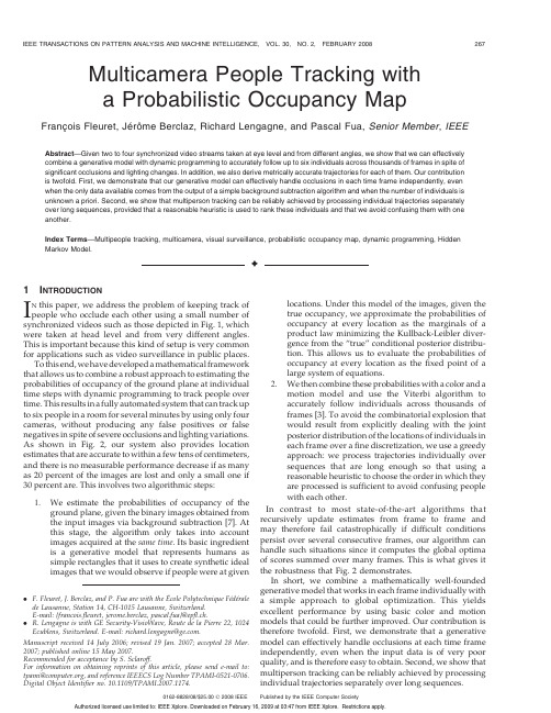
Multicamera People Tracking witha Probabilistic Occupancy MapFranc¸ois Fleuret,Je´roˆme Berclaz,Richard Lengagne,and Pascal Fua,Senior Member,IEEE Abstract—Given two to four synchronized video streams taken at eye level and from different angles,we show that we can effectively combine a generative model with dynamic programming to accurately follow up to six individuals across thousands of frames in spite of significant occlusions and lighting changes.In addition,we also derive metrically accurate trajectories for each of them.Our contribution is twofold.First,we demonstrate that our generative model can effectively handle occlusions in each time frame independently,even when the only data available comes from the output of a simple background subtraction algorithm and when the number of individuals is unknown a priori.Second,we show that multiperson tracking can be reliably achieved by processing individual trajectories separately over long sequences,provided that a reasonable heuristic is used to rank these individuals and that we avoid confusing them with one another.Index Terms—Multipeople tracking,multicamera,visual surveillance,probabilistic occupancy map,dynamic programming,Hidden Markov Model.Ç1I NTRODUCTIONI N this paper,we address the problem of keeping track of people who occlude each other using a small number of synchronized videos such as those depicted in Fig.1,which were taken at head level and from very different angles. This is important because this kind of setup is very common for applications such as video surveillance in public places.To this end,we have developed a mathematical framework that allows us to combine a robust approach to estimating the probabilities of occupancy of the ground plane at individual time steps with dynamic programming to track people over time.This results in a fully automated system that can track up to six people in a room for several minutes by using only four cameras,without producing any false positives or false negatives in spite of severe occlusions and lighting variations. As shown in Fig.2,our system also provides location estimates that are accurate to within a few tens of centimeters, and there is no measurable performance decrease if as many as20percent of the images are lost and only a small one if 30percent are.This involves two algorithmic steps:1.We estimate the probabilities of occupancy of theground plane,given the binary images obtained fromthe input images via background subtraction[7].Atthis stage,the algorithm only takes into accountimages acquired at the same time.Its basic ingredientis a generative model that represents humans assimple rectangles that it uses to create synthetic idealimages that we would observe if people were at givenlocations.Under this model of the images,given thetrue occupancy,we approximate the probabilities ofoccupancy at every location as the marginals of aproduct law minimizing the Kullback-Leibler diver-gence from the“true”conditional posterior distribu-tion.This allows us to evaluate the probabilities ofoccupancy at every location as the fixed point of alarge system of equations.2.We then combine these probabilities with a color and amotion model and use the Viterbi algorithm toaccurately follow individuals across thousands offrames[3].To avoid the combinatorial explosion thatwould result from explicitly dealing with the jointposterior distribution of the locations of individuals ineach frame over a fine discretization,we use a greedyapproach:we process trajectories individually oversequences that are long enough so that using areasonable heuristic to choose the order in which theyare processed is sufficient to avoid confusing peoplewith each other.In contrast to most state-of-the-art algorithms that recursively update estimates from frame to frame and may therefore fail catastrophically if difficult conditions persist over several consecutive frames,our algorithm can handle such situations since it computes the global optima of scores summed over many frames.This is what gives it the robustness that Fig.2demonstrates.In short,we combine a mathematically well-founded generative model that works in each frame individually with a simple approach to global optimization.This yields excellent performance by using basic color and motion models that could be further improved.Our contribution is therefore twofold.First,we demonstrate that a generative model can effectively handle occlusions at each time frame independently,even when the input data is of very poor quality,and is therefore easy to obtain.Second,we show that multiperson tracking can be reliably achieved by processing individual trajectories separately over long sequences.. F.Fleuret,J.Berclaz,and P.Fua are with the Ecole Polytechnique Fe´de´ralede Lausanne,Station14,CH-1015Lausanne,Switzerland.E-mail:{francois.fleuret,jerome.berclaz,pascal.fua}@epfl.ch..R.Lengagne is with GE Security-VisioWave,Route de la Pierre22,1024Ecublens,Switzerland.E-mail:richard.lengagne@.Manuscript received14July2006;revised19Jan.2007;accepted28Mar.2007;published online15May2007.Recommended for acceptance by S.Sclaroff.For information on obtaining reprints of this article,please send e-mail to:tpami@,and reference IEEECS Log Number TPAMI-0521-0706.Digital Object Identifier no.10.1109/TPAMI.2007.1174.0162-8828/08/$25.00ß2008IEEE Published by the IEEE Computer SocietyIn the remainder of the paper,we first briefly review related works.We then formulate our problem as estimat-ing the most probable state of a hidden Markov process and propose a model of the visible signal based on an estimate of an occupancy map in every time frame.Finally,we present our results on several long sequences.2R ELATED W ORKState-of-the-art methods can be divided into monocular and multiview approaches that we briefly review in this section.2.1Monocular ApproachesMonocular approaches rely on the input of a single camera to perform tracking.These methods provide a simple and easy-to-deploy setup but must compensate for the lack of 3D information in a single camera view.2.1.1Blob-Based MethodsMany algorithms rely on binary blobs extracted from single video[10],[5],[11].They combine shape analysis and tracking to locate people and maintain appearance models in order to track them,even in the presence of occlusions.The Bayesian Multiple-BLob tracker(BraMBLe)system[12],for example,is a multiblob tracker that generates a blob-likelihood based on a known background model and appearance models of the tracked people.It then uses a particle filter to implement the tracking for an unknown number of people.Approaches that track in a single view prior to computing correspondences across views extend this approach to multi camera setups.However,we view them as falling into the same category because they do not simultaneously exploit the information from multiple views.In[15],the limits of the field of view of each camera are computed in every other camera from motion information.When a person becomes visible in one camera,the system automatically searches for him in other views where he should be visible.In[4],a background/foreground segmentation is performed on calibrated images,followed by human shape extraction from foreground objects and feature point selection extraction. Feature points are tracked in a single view,and the system switches to another view when the current camera no longer has a good view of the person.2.1.2Color-Based MethodsTracking performance can be significantly increased by taking color into account.As shown in[6],the mean-shift pursuit technique based on a dissimilarity measure of color distributions can accurately track deformable objects in real time and in a monocular context.In[16],the images are segmented pixelwise into different classes,thus modeling people by continuously updated Gaussian mixtures.A standard tracking process is then performed using a Bayesian framework,which helps keep track of people,even when there are occlusions.In such a case,models of persons in front keep being updated, whereas the system stops updating occluded ones,which may cause trouble if their appearances have changed noticeably when they re-emerge.More recently,multiple humans have been simulta-neously detected and tracked in crowded scenes[20]by using Monte-Carlo-based methods to estimate their number and positions.In[23],multiple people are also detected and tracked in front of complex backgrounds by using mixture particle filters guided by people models learned by boosting.In[9],multicue3D object tracking is addressed by combining particle-filter-based Bayesian tracking and detection using learned spatiotemporal shapes.This ap-proach leads to impressive results but requires shape, texture,and image depth information as input.Finally, Smith et al.[25]propose a particle-filtering scheme that relies on Markov chain Monte Carlo(MCMC)optimization to handle entrances and departures.It also introduces a finer modeling of interactions between individuals as a product of pairwise potentials.2.2Multiview ApproachesDespite the effectiveness of such methods,the use of multiple cameras soon becomes necessary when one wishes to accurately detect and track multiple people and compute their precise3D locations in a complex environment. Occlusion handling is facilitated by using two sets of stereo color cameras[14].However,in most approaches that only take a set of2D views as input,occlusion is mainly handled by imposing temporal consistency in terms of a motion model,be it Kalman filtering or more general Markov models.As a result,these approaches may not always be able to recover if the process starts diverging.2.2.1Blob-Based MethodsIn[19],Kalman filtering is applied on3D points obtained by fusing in a least squares sense the image-to-world projections of points belonging to binary blobs.Similarly,in[1],a Kalman filter is used to simultaneously track in2D and3D,and objectFig.1.Images from two indoor and two outdoor multicamera video sequences that we use for our experiments.At each time step,we draw a box around people that we detect and assign to them an ID number that follows them throughout thesequence.Fig.2.Cumulative distributions of the position estimate error on a3,800-frame sequence(see Section6.4.1for details).locations are estimated through trajectory prediction during occlusion.In[8],a best hypothesis and a multiple-hypotheses approaches are compared to find people tracks from 3D locations obtained from foreground binary blobs ex-tracted from multiple calibrated views.In[21],a recursive Bayesian estimation approach is used to deal with occlusions while tracking multiple people in multiview.The algorithm tracks objects located in the intersections of2D visual angles,which are extracted from silhouettes obtained from different fixed views.When occlusion ambiguities occur,multiple occlusion hypotheses are generated,given predicted object states and previous hypotheses,and tested using a branch-and-merge strategy. The proposed framework is implemented using a customized particle filter to represent the distribution of object states.Recently,Morariu and Camps[17]proposed a method based on dimensionality reduction to learn a correspondence between the appearance of pedestrians across several views. This approach is able to cope with the severe occlusion in one view by exploiting the appearance of the same pedestrian on another view and the consistence across views.2.2.2Color-Based MethodsMittal and Davis[18]propose a system that segments,detects, and tracks multiple people in a scene by using a wide-baseline setup of up to16synchronized cameras.Intensity informa-tion is directly used to perform single-view pixel classifica-tion and match similarly labeled regions across views to derive3D people locations.Occlusion analysis is performed in two ways:First,during pixel classification,the computa-tion of prior probabilities takes occlusion into account. Second,evidence is gathered across cameras to compute a presence likelihood map on the ground plane that accounts for the visibility of each ground plane point in each view. Ground plane locations are then tracked over time by using a Kalman filter.In[13],individuals are tracked both in image planes and top view.The2D and3D positions of each individual are computed so as to maximize a joint probability defined as the product of a color-based appearance model and2D and 3D motion models derived from a Kalman filter.2.2.3Occupancy Map MethodsRecent techniques explicitly use a discretized occupancy map into which the objects detected in the camera images are back-projected.In[2],the authors rely on a standard detection of stereo disparities,which increase counters associated to square areas on the ground.A mixture of Gaussians is fitted to the resulting score map to estimate the likely location of individuals.This estimate is combined with a Kallman filter to model the motion.In[26],the occupancy map is computed with a standard visual hull procedure.One originality of the approach is to keep for each resulting connex component an upper and lower bound on the number of objects that it can contain. Based on motion consistency,the bounds on the various components are estimated at a certain time frame based on the bounds of the components at the previous time frame that spatially intersect with it.Although our own method shares many features with these techniques,it differs in two important respects that we will highlight:First,we combine the usual color and motion models with a sophisticated approach based on a generative model to estimating the probabilities of occu-pancy,which explicitly handles complex occlusion interac-tions between detected individuals,as will be discussed in Section5.Second,we rely on dynamic programming to ensure greater stability in challenging situations by simul-taneously handling multiple frames.3P ROBLEM F ORMULATIONOur goal is to track an a priori unknown number of people from a few synchronized video streams taken at head level. In this section,we formulate this problem as one of finding the most probable state of a hidden Markov process,given the set of images acquired at each time step,which we will refer to as a temporal frame.We then briefly outline the computation of the relevant probabilities by using the notations summarized in Tables1and2,which we also use in the following two sections to discuss in more details the actual computation of those probabilities.3.1Computing the Optimal TrajectoriesWe process the video sequences by batches of T¼100frames, each of which includes C images,and we compute the most likely trajectory for each individual.To achieve consistency over successive batches,we only keep the result on the first 10frames and slide our temporal window.This is illustrated in Fig.3.We discretize the visible part of the ground plane into a finite number G of regularly spaced2D locations and we introduce a virtual hidden location H that will be used to model entrances and departures from and into the visible area.For a given batch,let L t¼ðL1t;...;L NÃtÞbe the hidden stochastic processes standing for the locations of individuals, whether visible or not.The number NÃstands for the maximum allowable number of individuals in our world.It is large enough so that conditioning on the number of visible ones does not change the probability of a new individual entering the scene.The L n t variables therefore take values in f1;...;G;Hg.Given I t¼ðI1t;...;I C tÞ,the images acquired at time t for 1t T,our task is to find the values of L1;...;L T that maximizePðL1;...;L T j I1;...;I TÞ:ð1ÞAs will be discussed in Section 4.1,we compute this maximum a posteriori in a greedy way,processing one individual at a time,including the hidden ones who can move into the visible scene or not.For each one,the algorithm performs the computation,under the constraint that no individual can be at a visible location occupied by an individual already processed.In theory,this approach could lead to undesirable local minima,for example,by connecting the trajectories of two separate people.However,this does not happen often because our batches are sufficiently long.To further reduce the chances of this,we process individual trajectories in an order that depends on a reliability score so that the most reliable ones are computed first,thereby reducing the potential for confusion when processing the remaining ones. This order also ensures that if an individual remains in the hidden location,then all the other people present in the hidden location will also stay there and,therefore,do not need to be processed.FLEURET ET AL.:MULTICAMERA PEOPLE TRACKING WITH A PROBABILISTIC OCCUPANCY MAP269Our experimental results show that our method does not suffer from the usual weaknesses of greedy algorithms such as a tendency to get caught in bad local minima.We thereforebelieve that it compares very favorably to stochastic optimization techniques in general and more specifically particle filtering,which usually requires careful tuning of metaparameters.3.2Stochastic ModelingWe will show in Section 4.2that since we process individual trajectories,the whole approach only requires us to define avalid motion model P ðL n t þ1j L nt ¼k Þand a sound appearance model P ðI t j L n t ¼k Þ.The motion model P ðL n t þ1j L nt ¼k Þ,which will be intro-duced in Section 4.3,is a distribution into a disc of limited radiusandcenter k ,whichcorresponds toalooseboundonthe maximum speed of a walking human.Entrance into the scene and departure from it are naturally modeled,thanks to the270IEEE TRANSACTIONS ON PATTERN ANALYSIS AND MACHINE INTELLIGENCE,VOL.30,NO.2,FEBRUARY 2008TABLE 2Notations (RandomQuantities)Fig.3.Video sequences are processed by batch of 100frames.Only the first 10percent of the optimization result is kept and the rest is discarded.The temporal window is then slid forward and the optimiza-tion is repeated on the new window.TABLE 1Notations (DeterministicQuantities)hiddenlocation H,forwhichweextendthemotionmodel.The probabilities to enter and to leave are similar to the transition probabilities between different ground plane locations.In Section4.4,we will show that the appearance model PðI t j L n t¼kÞcan be decomposed into two terms.The first, described in Section4.5,is a very generic color-histogram-based model for each individual.The second,described in Section5,approximates the marginal conditional probabil-ities of occupancy of the ground plane,given the results of a background subtractionalgorithm,in allviewsacquired atthe same time.This approximation is obtained by minimizing the Kullback-Leibler divergence between a product law and the true posterior.We show that this is equivalent to computing the marginal probabilities of occupancy so that under the product law,the images obtained by putting rectangles of human sizes at occupied locations are likely to be similar to the images actually produced by the background subtraction.This represents a departure from more classical ap-proaches to estimating probabilities of occupancy that rely on computing a visual hull[26].Such approaches tend to be pessimistic and do not exploit trade-offs between the presence of people at different locations.For instance,if due to noise in one camera,a person is not seen in a particular view,then he would be discarded,even if he were seen in all others.By contrast,in our probabilistic framework,sufficient evidence might be present to detect him.Similarly,the presence of someone at a specific location creates an occlusion that hides the presence behind,which is not accounted for by the hull techniques but is by our approach.Since these marginal probabilities are computed indepen-dently at each time step,they say nothing about identity or correspondence with past frames.The appearance similarity is entirely conveyed by the color histograms,which has experimentally proved sufficient for our purposes.4C OMPUTATION OF THE T RAJECTORIESIn Section4.1,we break the global optimization of several people’s trajectories into the estimation of optimal individual trajectories.In Section 4.2,we show how this can be performed using the classical Viterbi’s algorithm based on dynamic programming.This requires a motion model given in Section 4.3and an appearance model described in Section4.4,which combines a color model given in Section4.5 and a sophisticated estimation of the ground plane occu-pancy detailed in Section5.We partition the visible area into a regular grid of G locations,as shown in Figs.5c and6,and from the camera calibration,we define for each camera c a family of rectangular shapes A c1;...;A c G,which correspond to crude human silhouettes of height175cm and width50cm located at every position on the grid.4.1Multiple TrajectoriesRecall that we denote by L n¼ðL n1;...;L n TÞthe trajectory of individual n.Given a batch of T temporal frames I¼ðI1;...;I TÞ,we want to maximize the posterior conditional probability:PðL1¼l1;...;L NÃ¼l NÃj IÞ¼PðL1¼l1j IÞY NÃn¼2P L n¼l n j I;L1¼l1;...;L nÀ1¼l nÀ1ÀÁ:ð2ÞSimultaneous optimization of all the L i s would beintractable.Instead,we optimize one trajectory after theother,which amounts to looking for^l1¼arg maxlPðL1¼l j IÞ;ð3Þ^l2¼arg maxlPðL2¼l j I;L1¼^l1Þ;ð4Þ...^l NÃ¼arg maxlPðL NÃ¼l j I;L1¼^l1;L2¼^l2;...Þ:ð5ÞNote that under our model,conditioning one trajectory,given other ones,simply means that it will go through noalready occupied location.In other words,PðL n¼l j I;L1¼^l1;...;L nÀ1¼^l nÀ1Þ¼PðL n¼l j I;8k<n;8t;L n t¼^l k tÞ;ð6Þwhich is PðL n¼l j IÞwith a reduced set of the admissiblegrid locations.Such a procedure is recursively correct:If all trajectoriesestimated up to step n are correct,then the conditioning onlyimproves the estimate of the optimal remaining trajectories.This would suffice if the image data were informative enoughso that locations could be unambiguously associated toindividuals.In practice,this is obviously rarely the case.Therefore,this greedy approach to optimization has un-desired side effects.For example,due to partly missinglocalization information for a given trajectory,the algorithmmight mistakenly start following another person’s trajectory.This is especially likely to happen if the tracked individualsare located close to each other.To avoid this kind of failure,we process the images bybatches of T¼100and first extend the trajectories that havebeen found with high confidence,as defined below,in theprevious batches.We then process the lower confidenceones.As a result,a trajectory that was problematic in thepast and is likely to be problematic in the current batch willbe optimized last and,thus,prevented from“stealing”somebody else’s location.Furthermore,this approachincreases the spatial constraints on such a trajectory whenwe finally get around to estimating it.We use as a confidence score the concordance of theestimated trajectories in the previous batches and thelocalization cue provided by the estimation of the probabil-istic occupancy map(POM)described in Section5.Moreprecisely,the score is the number of time frames where theestimated trajectory passes through a local maximum of theestimated probability of occupancy.When the POM does notdetect a person on a few frames,the score will naturallydecrease,indicating a deterioration of the localizationinformation.Since there is a high degree of overlappingbetween successive batches,the challenging segment of atrajectory,which is due to the failure of the backgroundsubtraction or change in illumination,for instance,is met inseveral batches before it actually happens during the10keptframes.Thus,the heuristic would have ranked the corre-sponding individual in the last ones to be processed whensuch problem occurs.FLEURET ET AL.:MULTICAMERA PEOPLE TRACKING WITH A PROBABILISTIC OCCUPANCY MAP2714.2Single TrajectoryLet us now consider only the trajectory L n ¼ðL n 1;...;L nT Þof individual n over T temporal frames.We are looking for thevalues ðl n 1;...;l nT Þin the subset of free locations of f 1;...;G;Hg .The initial location l n 1is either a known visible location if the individual is visible in the first frame of the batch or H if he is not.We therefore seek to maximizeP ðL n 1¼l n 1;...;L n T ¼l nt j I 1;...;I T Þ¼P ðI 1;L n 1¼l n 1;...;I T ;L n T ¼l nT ÞP ðI 1;...;I T Þ:ð7ÞSince the denominator is constant with respect to l n ,we simply maximize the numerator,that is,the probability of both the trajectories and the images.Let us introduce the maximum of the probability of both the observations and the trajectory ending up at location k at time t :Èt ðk Þ¼max l n 1;...;l nt À1P ðI 1;L n 1¼l n 1;...;I t ;L nt ¼k Þ:ð8ÞWe model jointly the processes L n t and I t with a hidden Markov model,that isP ðL n t þ1j L n t ;L n t À1;...Þ¼P ðL n t þ1j L nt Þð9ÞandP ðI t ;I t À1;...j L n t ;L nt À1;...Þ¼YtP ðI t j L n t Þ:ð10ÞUnder such a model,we have the classical recursive expressionÈt ðk Þ¼P ðI t j L n t ¼k Þ|ﬄﬄﬄﬄﬄﬄﬄﬄﬄ{zﬄﬄﬄﬄﬄﬄﬄﬄﬄ}Appearance modelmax P ðL n t ¼k j L nt À1¼ Þ|ﬄﬄﬄﬄﬄﬄﬄﬄﬄﬄﬄﬄﬄﬄﬄﬄﬄ{zﬄﬄﬄﬄﬄﬄﬄﬄﬄﬄﬄﬄﬄﬄﬄﬄﬄ}Motion modelÈt À1ð Þð11Þto perform a global search with dynamic programming,which yields the classic Viterbi algorithm.This is straight-forward,since the L n t s are in a finite set of cardinality G þ1.4.3Motion ModelWe chose a very simple and unconstrained motion model:P ðL n t ¼k j L nt À1¼ Þ¼1=Z Áe À k k À k if k k À k c 0otherwise ;&ð12Þwhere the constant tunes the average human walkingspeed,and c limits the maximum allowable speed.This probability is isotropic,decreases with the distance from location k ,and is zero for k k À k greater than a constantmaximum distance.We use a very loose maximum distance cof one square of the grid per frame,which corresponds to a speed of almost 12mph.We also define explicitly the probabilities of transitions to the parts of the scene that are connected to the hidden location H .This is a single door in the indoor sequences and all the contours of the visible area in the outdoor sequences in Fig.1.Thus,entrance and departure of individuals are taken care of naturally by the estimation of the maximum a posteriori trajectories.If there are enough evidence from the images that somebody enters or leaves the room,then this procedure will estimate that the optimal trajectory does so,and a person will be added to or removed from the visible area.4.4Appearance ModelFrom the input images I t ,we use background subtraction to produce binary masks B t such as those in Fig.4.We denote as T t the colors of the pixels inside the blobs and treat the rest of the images as background,which is ignored.Let X tk be a Boolean random variable standing for the presence of an individual at location k of the grid at time t .In Appendix B,we show thatP ðI t j L n t ¼k Þzﬄﬄﬄﬄﬄﬄﬄﬄﬄ}|ﬄﬄﬄﬄﬄﬄﬄﬄﬄ{Appearance model/P ðL n t ¼k j X kt ¼1;T t Þ|ﬄﬄﬄﬄﬄﬄﬄﬄﬄﬄﬄﬄﬄﬄﬄﬄﬄﬄ{zﬄﬄﬄﬄﬄﬄﬄﬄﬄﬄﬄﬄﬄﬄﬄﬄﬄﬄ}Color modelP ðX kt ¼1j B t Þ|ﬄﬄﬄﬄﬄﬄﬄﬄﬄﬄﬄ{zﬄﬄﬄﬄﬄﬄﬄﬄﬄﬄﬄ}Ground plane occupancy:ð13ÞThe ground plane occupancy term will be discussed in Section 5,and the color model term is computed as follows.4.5Color ModelWe assume that if someone is present at a certain location k ,then his presence influences the color of the pixels located at the intersection of the moving blobs and the rectangle A c k corresponding to the location k .We model that dependency as if the pixels were independent and identically distributed and followed a density in the red,green,and blue (RGB)space associated to the individual.This is far simpler than the color models used in either [18]or [13],which split the body area in several subparts with dedicated color distributions,but has proved sufficient in practice.If an individual n was present in the frames preceding the current batch,then we have an estimation for any camera c of his color distribution c n ,since we have previously collected the pixels in all frames at the locations272IEEE TRANSACTIONS ON PATTERN ANALYSIS AND MACHINE INTELLIGENCE,VOL.30,NO.2,FEBRUARY2008Fig.4.The color model relies on a stochastic modeling of the color of the pixels T c t ðk Þsampled in the intersection of the binary image B c t produced bythe background subtraction and the rectangle A ck corresponding to the location k .。

ABB DF23流量计

Data SheetD184S037U02FieldElectromagnetic FlowmeterFXF2000 (COPA-XF)with Pulsed DC Field Excitationin a Compact DesignIT ■Function–Electromagnetic flowmeters [EMF] can be used to accurately measure the flowrate of liquids, pulps, slurries and sludges with a minimum fluid conductiv-ity of ≥ 5 µS/cm ■Applications–Suitable for flow measurements in batch and fill operations as well as for continuous flow metering –The compact design of the EMF allows cluster mounting where minimal space requirements exist –Compact design made completely of stainless steel –Reproducibility ± 0.2 % of rate–The supply power and the output signal connections of the converter are made using a single cable with plug–Easy cleaning and sterilization – including automated CIP/SIP-systems – require a smooth, unrestricted meter pipe in the flowmeter primary –Certifications per FDA, EHEDG, 3A ■Communication–Optional 2nd communication plug –ASCII-Protocol (RS 485)■Multiple Operating Modes–Continuous flow metering with current/pulse output –Flowmeter sensor with a frequency output –Stand-Alone batch and fill system operation…All in one“ - FlowmeterCompact plus High PerformanceOverview of the Flowmeter Primary and Converter Designs Overview, Process Connections2Accuracy, Reference Conditions and Operating PrincipleDesignThe Electromagnetic Flowmeters in the Compact Design occupy a spe-cial niche. In this design, the converter is mounted directly on the flow-meter primary. This appreciably decreases installation costs because a signal cable is no longer required between the flowmeter primary and the converter.Operating PrincipleThe operation of the electromagnetic flowmeter is based on Faraday’s Laws of Induction. A voltage is generated in a conductor as it moves through a magnetic field.This measurement principle is applied to a conductive fluid which flows in a pipe through which a magnetic field is generated perpendicular to the flow direction (see Schematic Fig. 1: ).The signal voltage which is induced in the fluid is measured at two elec-trodes located diametrically opposite to each other. This signal voltage U E is proportional to the magnetic induction B, the electrode spacing D and the average fluid velocity v.Noting that the magnetic induction B and the electrode spacing D are constant values, indicates that a proportionality exists between the signal voltage U E and the average flow velocity v. The equation for calculating the volumetric flowrate shows that the signal voltage U E is linear and proportional to the volumetric flowrate.Reference Conditions per EN 29104FluidWater, conductivity 200 µS/cm ± 10 %Fluid Temperature20 °C ± 2 KAmbient Temperature20 °C ± 2 KSupply PowerNominal voltage U N ±1 %Installation Requirements, Straight Pipe Sections Upstream >10xDDownstream >5xDD = Flowmeter primary sizeWarm Up Time≥ 30 MinutesEffect on Analog OutputSame as pulse output plus ± 0.1 % of rateReproducibility – Fill OperationsThe constant boundary conditions which exist for these applications allow replacing the above instrument/system accuracy (± 0.5 % of rate) Fig. 2: , with fill operation accuracies of:± 0.2 % for T Filll≥ 4 s± 0.4 % for 2 s ≤ T Filll≤ 4 s(standard accuracy)Reproducibility – Continuous Flow Metering± 0.2 % of rate3Converter Specifications/Operating Modes 50XF4000Supply Power24 V DCContact Outputs - Optocoupler (see specific Variant)–Pulse/frequency output–Alarm contact–Forward/reverse direction signal–Synchronized output–End contactAnalog Output–Current outputContact Inputs - Optocoupler (see specific Variant)–Ext. zero return–System zero–Synchronized input–Start/stop inputData Link/ Protocol–RS 485 / ASCII–RS 485 / ASCII 2wDetector Empty PipeOperating Modes–Standard continuous.–Conti1kHz–Conti2kHz–Conti5kHz–Standard batch–Batch 1 kHz–Batch 2 kHz–Batch 5 kHz–Fill 5 kHzPlug ConnectionsConfigure Using–Operator Unit 55BE1000–Handheld Terminal 55HT4000Approvals / Certifications–3A-Certificate–FDA–EHEDG-Certificate Operating Modes, FXF2000 (COPA-XF)In addition to continuous flow metering with current and pulse outputs, the following operating modes are available.Flow Sensor for a Higher Level Fill Control Systemas a Stand-Alone “Filler” with integrated Fill-Software4Meter Size Table, Flow Ranges,Flowrate NomographMeter Size, Pressure Rating (Weld Stubs)and Flow Ranges1)Values for other process connections see Page 2Effective Flow Velocity, Variable Process Connections, PFA Flowrate NomographThe volume flowrate is a function of both the flow velocity and the flow-meter size. The Flowrate Nomograph, Fig. 5 shows the flow range appli-cable to each flowmeter size as well as the flowmeter sizes suitable for a specific flowrate.Example:Flowrate = 120 l/min (maximum value = flow range end value). SuitableMeter size DN InchStd.Press. RatingPN1)min.Flow RangeFlow Velocity0 to 0.5 m/smin.Flow RangeFlow Velocity0 to 10 m/s3 4 61/105/321/44040400 to0.2l/min0 to0.4l/min0 to1l/min0 to4l/min0 to8l/min0 to20l/min8 10 155/163/81/24040400 to 1.5l/min0 to 2.25l/min0 to5l/min0 to30l/min0 to45l/min0 to100l/min20 25 323/411¼4040400 to7.5l/min0 to10l/min0 to20l/min0 to150l/min0 to200l/min0 to400l/min40 50 651½22½4016100 to30l/min0 to3m3/h0 to6m3/h0 to600l/min0 to60m3/h0 to120m3/h80 1003416100 to9m3/h0 to12m3/h0 to180m3/h0 to240m3/hMeter SizeDN InchCal-Fac [l/min]d eff [mm]Q d eff [l/min]V eff [m/s]31/1043 4.29.445/32847.510.661/4 20 6 17.011.885/16 30 8 30.2 9.9103/8 4510 47.1 9.5151/2 10013 79.612.6203/4 15018 152.7 9.8251 20024 271.4 7.4321¼ 40030 424.1 9.4401½ 60036 610.7 9.85021000471041.0 9.6652½2000621811.411.08033000742580.511.610044000964342.9 9.25Installation Requirements,Flowmeter Primary DF23In-/Outlet Straight SectionsThe measurement principle is independent of the velocity profile as long as standing eddies do no extend into the measurement zone, e.g., after double elbows, tangential inflow or partially opened gate valves upstream of the flowmeter primary. In such situations measures should be em-ployed to normalize the flow profile.Straight sections with the same diameter as the flowmeter primary should be installed upstream and downstream. The straight length up-stream of the flowmeter primary should be of at least 10 times the diam-eter of the flowmeter primary and downstream at least 5 times. Experience has indicated that in most of the installations a straight inlet section of 3xD and a straight outlet section of 2xD is sufficient.Installation of the Flowmeter PrimaryThe flow direction should be considered during installation (fluid flows into the plug connection socket), because the flowmeter should be operated in the forward direction if possible. The flow direction for the measure-ments can be reversed using the software, if required. Generally, the con-nection plug socket should point downward for vertical installations. The flowmeter must be installed so that the meter pipe is always completely filled with fluid. Valves or other shut off devices should be installed down-stream to prevent the flowmeter primary from draining.GroundingGrounding the electromagnetic flowmeter primary is not only essential for safety reasons but also to assure proper operation. The ground screw on the flowmeter primary, for measurement reasons, is to be connected to earth. An additional ground to the connection plug is not required.For plastic or lined (with electrically insulating liners) pipelines the ground is made using a grounding plate or grounding electrode. If stray currents are present in the pipeline, it is recommended that grounding plates be installed up- and downstream of the flowmeter primary.Connection CablesAttentionThe flowmeter primary should not be installed near equipmentwith strong electromagnetic fields. A shielded interconnectioncable is recommended. It is beneficial to route the cables in met-al conduit, in which a number of cables of the same type can beinstalled together in a single conduit.Extra cable should not be coiled.Appropriate noise reduction measures should be employed, e.g., protec-tion diodes, varistors or R-C combinations (VDE 0580) for valves or con-trol switches located in the vicinity of the flowmeter system.InformationThe instrument conforms to the requirements in the EMC-Direc-tive and the NAMUR-Recommendations NE 21 3/93 “Electro-magnetic Compatibility of Equipment in Processes and Labora-tories”.InformationWhen installing the cable to the flowmeter primary, a water trapshould be provided.Output SignalsThe flowrate proportional frequency / scaled pulse output can be con-nected to an electronic counter, a SPC, a PC or a process control sys-tem. Therefore it is possible to integrate the flowmeter primary in a batch or fill system as well as utilize it in continuous flow processes.The pulse output in batch and fill operations must be processed by other peripheral instruments. This includes the control of the system, integrat-ing the flow, actuating the valves when the batch quantity is reached, cal-culating the second stage flow and monitoring the over- or under fills. A low flow cutoff feature can be turned on if required. Optionally, the inte-grated batch software can be used for single stage fill operations. Additionally, in the operating modes “Conti”, a 0/4–20 mA current output is available.Electrode AxisFor horizontal installations assure that neither of the two electrodes are located at the highest point. Any gas bubbles present in the fluid could accumulate and interrupt the electrical connection between the electrode and the fluid. The ideal installation for an EMF is assured in vertical pipe-67Installations in Larger Size PipelinesThe flowmeter primary can readily be installed in larger pipeline sizes by utilizing reducers (e.g. flanged reducers DIN 28545). The pressure drop which results from the reduction can be determined from the Nomograph Fig. 7: The pressure drop is determined in the following manner:1.Calculate the diameter ratio d/D.2.Calculate the flow velocity as a function of the flowmeter sizeand the flowrate :v =The flow velocity can also be determined from the Flowrate Nomograph Fig. 5: 3.In Fig. 7: the “Pressure Drop” can be read on the Y-axis at theintersection of the flow velocity value and the “Diameter Ratio” (X-axis) value.Specifications, Flowmeter Primary DF23Min. Allowable Absolute Pressure as a Function of the Fluid TemperatureMax. Allowable Fluid Temperature and PressureMax. Allowable Cleaning Temperature PFA-DesignIf the ambient temperature >25 °C, the difference is to be subtracted from the max. cleaning temperature.T max - °C, where °C = (T amb. -25 °C).Max. Allowable Shock TemperatureAmbient RequirementsAmbient Temperature -20 °C to +60 °CFluid Temperature-25 °C to +130 °C, CIP-cleanable, see Temperature Diagram and max. allowable cleaning temperature.Maximum allowable ambient temperature as a function of the fluid temperature for stainless steel process connections and Wafer De-Q (instantaneous flowrate)PrimaryConstant-----------------------------------------------------------LinerMeter SizeDNInchP Operate mbar absat T Operate °C PFA3 – 100 1/10 – 4≤130Process connections Liner PFAMeter SizeDNInchP Operate bar at T Operate °C Wafer Design,Weld stubs DIN 11850Weld stubs DIN 24633- 1001/10- 410–40≤130Weld stubs ISO 203725-1001- 410–40≤130Food Ind. fittings DIN 118513- 401/10-1½ 50-1002- 44025≤≤130130Tri-Clamp DIN 326763- 1001/10- 410–16≤130Fixed-Clamp 10- 403/8-1½10≤130External threads ISO 228 / DIN 29993- 251/10- 110≤130CIP-CleaningLiner T max °C T max minutes T amb °C Steam cleaning orLiquid cleaningPFA15014060602525Liner Temp.-Shock Max. Temp.-Diff. °CTemp.-Gradient°C/minPFAanyany∆∆8Storage Temperature -25 °C to +70 °CVariant Overview Series 2000 (Stainless Steel Design) Material Load Curves for Wafer Design Instrument Model DF23Materials, Flowmeter PrimaryProcess Connection MaterialGasket Materials, Electrical Connections, Weight and DesignSupply Power From converterWeightSee Dimensions Pages 9 – 13DesignFlowmeter primary with integrated µP-converterFlowmeter primary and converter housing in stn. stl. 1.4301 [304]Process Connections DN 3 – 100 [1/10” – 4”]See Page 2 and Pages 9 – 13Protection ClassStandard IP 67, option tropicalized Max. Pipeline Vibration15 m/s 2 (1.5 g) for f = 10 – 150 HzMax. Allowable Fluid Temperature and Pressure Process Connections DF23*)Higher temperatures for CIP/SIP cleaning are allowed for restricted time periods, see Table …Max. allow. Cleaning Temperature“Model:DF23B E T R Q P S F WM e t e r S i z eP r o c e s s C o n n ’s1/8“-S a n i t a r y c o n n ’sE x t e r n a l t h r e a d sT r i -C l a m p D I N 32676W e l d s t u b s D I N 11850W e l d s t u b s D I N 2463W e l d s t u b s I S O 2037F o o d I n d . f i t t i n g D I N 11851F l a n g e sW a f e r D e s i g n11/25x PED[DGRL]21/12xS E P S e c t . 3,P a r . 331/10x x x x x x x 45/32x x x x x x x 61/4x x x x x x x 85/16x x x x x x x 103/8x x x x x x x 151/2x x x x x x x 203/4x x x x x x x 251xx x x x x x x 321-1/4x x x x x x x C o n f o r m i t y p e r C a t e g o r y I I I M o d u l e B 1+D ,F l u i d G r o u p 1401-1/2x x x x x x x 502x x x x x x x 652-1/2x x x x x x x 803x x x x x x x 1004xxxxxxxLiner Material Electrode Material Electrode Design Standard OthersStandardOthers PFAHast.-C4(1.4539 for weld stubs, Food Ind. fittings & Tri-Clamp)SS 1.4539SS1.4571[316Ti] Tantalum, TitaniumFlat head Pointed head (≥ DN10 [3/8”])StandardOptionWafer Design NoneWeld stubs SS 1.4404 [316L]SS 1.4435 [316L]Food Ind. fittingDIN 11851SS 1.4404 [316L]SS 1.4435 [316L]Tri-Clamp DIN 32676SS 1.4404 [316L]SS 1.4435 [316L]Fixed-Clamp SS 1.4404 [316L]SS 1.4435 [316L]External threadsSS 1.4404 [316L]SS 1.4435 [316L]Process Connection Materials Gasket Materials Wafer Design noneWeld stubs Food Ind. fitting Tri-Clamp Fixed-Clamp External threads EPDM (Ethylene-Propylene) std. with FDA-ApprovalSilicone with FDA-Approval (option)Flat housing gasketSiliconeProcess Connections Liner PFA Meter Size DN Inch PSbar at TS °C Wafer Design 3–501/10-2 65–1002½-44016≤≤130*)130*)Weld stubs 3–401/10-1½50, 802, 365, 1002½, 4401610≤≤≤130*)130*)130*)Tri-Clamp3–501/10-265–1002½-41610≤≤121121Food Ind. fittings 3–401/10-1½50, 802, 365, 1002½, 4401610≤≤≤130*)130*)130*)External threads 3–251/10-110≤130*)Fixed-Clamp 10–403/8-1½10≤130*)DN Inch910Specifications, ConverterFlow RangeSelectable between 0.05 – 1* Cal-FacReproducibility0.2 % for T Fill≥ 4 s0.4 % for 2 s ≤ T Fill≤ 4 sFlow DirectionForward/reverseMinimum Conductivity≥ 5 µS/cm, ≥ 20 µS/cm DN 3 - 8 [1/10” - 3/16”],≥ 20 µS/cm deionized waterElectrical Connections8-pin plug (supply power, signals)4-pin plug (data link RS485 - option)Supply Power24 V DC, allowable voltage deviations +/-30 %Ripple ≤ 5 %PowerDN 3 to DN 100 [1/10” to 4”] ≤ 6 W (flowmeter primary incl. converter) Magnetic Field Excitation12.5 Hz / 25 HzAmbient Temperature-20 °C to +60 °C (see also Temperature Diagram Fig. 8: ) Response Time for Pulse-/Frequency OutputsMin. response time T0/99 =Min. fill time T Fill = 2 sLow Flow CutoffSelectable from 0 to 10 % of max.Output Signals–Scaled pulse output,passive, optocoupler0 ≤ U CEL≤ 2 V; 16 V ≤ U CEH≤ 30 V2 mA ≤ I CEL≤ 220 mA; 0.2 mA ≤ I CEH≤ 2 mASetting range: 0.001 – 1000 pulses per selected unitPulse width: 100s – 2000 msfmax : 5 kHzPIN 3 and 4–Flowrate proportional frequency output1.2 or 5 kHz for flowrate = 100 %passive, optocoupler0 ≤ U CEL≤ 2 V; 16 V ≤ U CEH≤ 30 V2 mA ≤ I CEL≤ 220 mA; 0.2 mA ≤ I CEH≤ 2 mAPIN 3 and 4–Current output (selectable)Load ≤ 600 for 0/4–20 mA, 0–10– 20 mA, 4–12–20 mALoad ≤ 1200 for 0/2–10 mALoad ≤ 2400 for 0–5 mAPIN 5 and 8–Data link RS 485Max. cable length 1200 mMax. no. of instruments: 32 Instruments in parallelMax. baudrate: 9600 BaudCommunication-Protocol: ASCII 2W“Communication plug” PIN 3 and 4Connection to Handheld-Terminal or SPC, PCS, PC –Handheld Terminal 55HT4000Plug into “Communication Plug Socket”Supply power 24 V DC over PIN 1 and 2–Contact output (function of operating mode) Alarm, forward/reverse, synchronized or end contact passive, optocoupler0 ≤ U CEL≤ 2 V; 16 V ≤ U CEH≤ 30 V0 mA ≤ I CEH≤ 0.2 mA, 2 mA ≤ I CEL≤ 220 mAPIN 1 and 3–Contact input (function of operating mode) Ext. zero return, system zero, synchronized input,Start/stop inputOptocoupler16 V ≤ U ≤ 30 V, R i = 2 kOhmPIN 5 and 21MagneticFieldExcitation---------------------------------------------------------------µΩΩΩOverview, Possible Converter VariantsLegends: x Default setting o Selectable A, B, K Only selectable for specific operating mode. Design Level BVariant0207Hardware Contact output x x Contact input x x Pulse passive x x Current output xRS 485xMenusOperating mode Standard conti.K x x Standard Batch B o o Batch 1 kHz B1o o Batch 2 kHz B2o o Batch 5 kHz B5o o Filler 5 kHz A o o Conti 1 kHz K1o o Conti 2 kHz K2o o Conti 5 kHz K5o o Contact output Alarm x x Fwd./Rev.o o Synchronized o o End contact A A Contact input Ext. zero return x x System zero o o StartAA Current outputK K1K2K5Data link ASCII x ASCII2w o DEP K KPlug TypePIN-Assignments for the Standard Plug FXF2000Assignments Communication Plug Variant PIN 1PIN 2PIN 3PIN 4PIN 5PIN 6PIN 7PIN 8PIN 1PIN 2PIN 3PIN 42P7G2Ux V8X1U+U-../..+ 25 V B A 7P7X1Ux V8+U+U-–../..../..../..../..Customer Specific Variant 20P7../..Ux V8+U+U-–+ 25 V B A 21P7G2Ux V8X1U+U-../..../..../..../..../..22P7Vc Ux V8+U+U-–../..../..../..../..23P7G2Ux V8X1U+U-Air../..../..../..../..⊥⊥Interconnection Diagram FXF2000, High-Side Switching, Model DF23, Design Level BDesign High-Side Switching(Pulse output, current output, contact input, contact output, supply power, data link, supply power, handheld terminal) a)Scaled pulse output, passive optocoupler, pulse width selectable from 0.100 ms to 2000 ms fmax 5 kHz as a function of the selection in the submenu “Operating mode”, 0 V ≤ U CEL ≤ 2 V, 16 V ≤ U CEH ≤ 30 V2 mA ≤ I CEL ≤ 220 mA; 0.2 mA ≤ I CEH ≤ 2 mAConnection plug assignments PIN 3, 4; Function Ux, V8d)Current output (selectable)Load ≤ 600 for 0/4–20 mA, 0–10– 20 mA, 4–12–20 mA Load ≤ 1200 for 0/2–10 mA; load ≤ 2400 for 0–5 mA Connection plug assignments PIN 5 and 8; Function +, –e)Contact output, function selectable dependent upon the selection in the submenu “Operating mode”, Synchronized signal (output signal synchronized to the excitation), F/R signal or end contact,passive optocoupler, 0 V ≤ U CEL 2 V, 16 V ≤ U CEH ≤ 30 V / 0 mA ≤ I CEH ≤ 0.2 mA, 2 mA ≤ I CEL ≤ 220 mA Connection plug assignments PIN 1, 3; Function P7, Uxf)Contact input, function selectable dependent upon the selection in the submenu “Operating mode”, Start/Stop, external totalizer reset, system zero 1), no function, passive optocoupler, 16 V ≤ U ≤ 30 V, Ri = 2 kOhm Connection plug assignments PIN 2, 5; Function G2, X1g)Supply power 24 V DC ± 30 %, ripple ≤ 5 %Connection plug assignments PIN 6, 7; Function U+, U-i)Data link RS 485, 2-Wire, V PP = 5 V, input resistance ≥ 12 kOhmmax. cable length ≤ 1200 m, shielded cable with twisted pairs required, Baudrate 110 - 9600 Baud, max. 32 instruments in parallel,Communication plug assignments PIN 3, 4; Function B, A (RS 485)j)Connection for Handheld Terminal 55HT4000Communication plug assignments PIN 3, 4; Function B, A (RS 485);Communication plug assignments PIN 1, 2; Function , +25 V (supply power for 55HT4000)1)Initiates a system zero adjustment procedure.The fluid must be at absolute zero flowrate and the meter pipe must be completely ment:To maintain the EMC-Requirements the instrument must be connected to earth. When the housing is opened the EMC-Protection is voided.Assignment Connection Plug Communication {Plug PIN-No.123456781234Legends Functions (PIN-Assignments)Functions (PIN-Assignments)a)Ux V8d)+–e)P7Ux f)G2X1g)U+U-i)B A j)+25V B A ⊥ΩΩΩ⊥Fig. 15:Interconnection Diagram, High-Side Switching, In-/Outputs with PIN-Assignments for the Connection and Communication PlugsInterconnection Examples for Peripherals FXF2000 (COPA-XF), Model DF23, High-Side Switching, In-/Outputs/Data LinkVariant Overview High-Side Switching and SPC-ConformityVariant: 2, 21, 23High-side switching SPC conf.Variant: 20 High-side switching SPC conf.Variant: 7High-side switchingPulse outputInputContact output X1 (5)G2 (2)UX (3)P7 (1)V8 (4)V8 (4)– (8)+ (5)P7 (1)UX (3)X1 (2)InputPulse outputContact output Current outputactivePulse outputContact outputV8 (4)P7 (1)Vc (2)UX (3)2nd Pulse outputCurrent output– (8)+ (5)active – (8)+ (5)V8 (4)UX (3)P7 (1)Pulse outputContact outputCurrent output activeVariant: 22High-side switching SPC conf.Fig. 17:Variant Overview High-Side Switching and SPC-ConformityInterconnection Diagram FXF2000, High-Side Switching/Plug with Installed Cable, Model DF23,Ordering Information: Electromagnetic Flowmeter Model DF23In addition to the Ordering Number, please include the following information: Fluid, fluid temperature, operating pressure, pipeline design (grounding plates) 1)Installation accessories see Table H in the Price List 2)Grounding electrodes from DN 3 [1/10”]Compact Design FXF2000 (COPA-XF)DF23Process ConnectionsWafer Design 1)Weld stubs DIN 11850(standard)Weld stubs DIN 2463Weld stubs ISO 2037 (DN 25-100 [1” - 4”]) Food Ind. fitting DIN 11851Tri-Clamp DIN 32676Fixed-Clamp (DN 10-40 [3/8”-1½”]) External threads ISO 228/DIN 2999(DN 3-25 [1/10” - 1”]) Without adapter (no coupling nut or screws)W R Q PS T C EV Liner Material PFA P Meter SizeDN 31/10”DN 45/32”DN 61/4”DN 85/16”DN 103/8”DN 151/2”DN 203/4”DN 251”DN 321¼”DN 401½DN 502”DN 652½”DN 803”DN 1004”030406081015202532405065801H Signal ElectrodeMaterial / Ground Electrode Material 2)Stn. stl. (1.4539)/ none (standard)Stn. stl. (1.4571[316Ti])/ noneHastelloy C-4 (2.4610)/ noneTitanium / noneTantalum / noneF S H M T Stn. stl. (1.4539)/ with (standard)Stn. stl. (1.4571[316Ti])/ withHastelloy C-4 (2.4610)/ withTitanium / withTantalum / withR E O I Q Pressure Rating PN 10Tri-Clamp (DN 65-100 [2½”- 4”]), External threads/Food Ind. fitting/Weld stubs (DN 65, 100 [2½”, 4”])PN 16Wafer Design/Tri-Clamp (DN 3-50 [1/10”-2”]), Food Ind. fitting/Weld stubs (DN 50, 80 [2”,3”])PN 40Wafer Design (DN 3-50 [1/10”-2”]), Food Ind. fitting/Weld stubs (DN 3-40 [1/10”-1½”])C D F JIS K10Wafer Design DN 3-100 [1/10” - 4”] ANSI CL 150Wafer Design DN 3-100 [1/10” - 4”] ANSI CL 300Wafer Design DN 3-50 [1/10” - 2”]K P QProcess Connection Materials None (only Wafer Design) Stn. stl. 1.4404[316L)(standard)04Accessories None (standard) With instrument mounting element A CTemperature Range Standard design <130 °C SCertifications None (standard)Material Traceability Certificate 3.1B per EN 10204 and Pressure Test per AD-2000 Inspection Report per EN 10204 3.1B Pressure Test per AD-2000A D F G3) Variant No. ≥ 20: customer specific Variant4) For use in applications with high grease contentAttentionTo configure the converter the Operator Unit 55BE1000 is required and the housing cover must be removed.ATTENTION! When the housing cover is removed the EMC-Protection is limited.If a data link option is included in the converter, the converter can be configured without removing the cover from a Handheld Terminal 55HT4000, PCS-System or PC using the ASCII-Protocol.Compact Dsg. FXF2000 (COPA-XF) DF23Protection Class IP 67 Standard) Tropicalized 24Supply Power 24 V DC H External Connections Connection plug (angled),(standard) (for Variant selection 07) Connection plug (angled),plus communication socket and plug (for Variant selection 02)16In-/Outputs (Variant) 3)(see External Connections)Contact output /pulse passive, opto /contact input/RS 485 (2nd plug) (6) Contact output /pulse passive, opto /contact input/current output (standard) (1)0207Application StandardFactory Plate German EnglishG EDesign Level BGasket MaterialsEPDM with FDA-Approval (standard) Silicone with FDA-Approval (option) None (only Wafer Design)E S OElectrode Design StandardPointed head 4)(from DN 10 [3/8”])12Ordering Information Operator Unit 55BE1000 Ordering Number55BE1DesignWith 9 V battery for lighting the display10A Factory PlateGerman English 1 22122Ordering Information Handheld Terminal 55HT4000Ordering Number55HT4Keypad LayoutStandard1Supply Power 24 V AC/DC1Connection Cable with Plug2.5 m with straight plug, Handheld Terminal10 m with angle plug, for panel mounting12Design Level0Factory PlateGermanEnglish 12Fig. 20:Handheld Terminal 55HT4000 for Data Entry.A prerequisite is a FXF2000 design which includesa data link RS 485 and a communication plug socketD 184S 037U 02 R e v . 02The Industrial IT wordmark and all mentioned product names in the form XXXXXX IT are registered or pending trademarks of ABB.ABB has Sales & Customer Support expertise in over 100 countries worldwide.The Company’s policy is one of continuous product improvement and the right is reserved to modify the information contained herein without notice.Printed in the Fed. Rep. of Germany (03.04)© ABB 2004ABB Ltd.Oldends Lane, Stonehouse Gloucestershire, GL 10 3TA UK Phone:+44(0)1453 826661Fax:+44(0)1453 829671ABB Inc.125 E. County Line Road Warminster, PA 18974USA Phone:+1 215 674 6000Fax:+1 215 674 7183ABB Automation Products GmbH Dransfelder Str. 237079 GöttingenGERMANYPhone:+49 551 905-534Fax:+49 551 905-555CCC-support.deapr@。

流式计数Accuri-TB-Guide-to-Absolute-Counting

BD Biosciences January 2012
Technical Bulletin A Guide to Absolute Counting Using the BD Accuri™ C6 Flow Cytometer
Page 3
5. Within 5 minutes of completing the water run, place a calibration sample on the SIP. Select Instrument > Calibrate Fluidics. • Calibration should be performed in the same tube type as the experimental sample. • Calibration should be performed using a sample of the same or similar viscosity as the samples to be analyzed. For example, if lysed human peripheral blood samples are to be acquired, lysed human peripheral blood should be used during calibration. • The calibration procedure consumes approximately 220 µL. To account for this, the volume in the calibration sample tube should be 110 µL more than the average volume used with subsequent test samples. For example, if using 1,000-µL samples, perform calibration with 1,110 µL in the tube. The values determined by the BD Accuri C6 are based on the average sample height in the tube during the calibration. • If sample volumes >50 µL are to be acquired from the sample tube, the calibration volume should take this into account and the average volume in the sample tube during the acquisition should be used. For example, if 100 µL is to be acquired from a 1,000-µL sample, the average volume would be 950 µL.

Flow 研究概述

以上是 Flow 结构的一般理论模型，目前随着对 Flow 研究的进一步深入，某些应用领域也出现了一些新的结构模型，如人机交互中的 Flow 因果结构模型等（Novak, 1997）。
3 Flow 的特征和产生条件
研究表明，Flow 心理体验的产生具有跨阶层性、跨性别性、跨年龄性、跨活动性和一定的跨文化性（Sedig，2007）。处于 Flow 状态中的个体几乎都有以下几个共同特征：（1）体验活动本身成为活动的内在动机；（2）个体的注意力高度集中于当前所从事的活动，任何其他的外在引诱最多也只可能使个体出现暂时的分心；（3）自我意识的暂时丧失，如忘记了自己的社会身份、忘记了自己的身体状况（饥饿、疲劳）等；（4）行动与意识相融合；（5）出现暂时性体验失真，较典型的如觉得时间过得比平常要快；（6）对当前的活动具有较好的控制感，即一个人能大致认识到自己能应对即将出现的后续行为并能对它做出适当的反应；（7）具有直接的即时反馈，活动的每一个环节都是对上一活动环节的反馈；（8）个体所感知到的活动的挑战性和自身的技能水平间具有平衡性；（9）有明确的活动目标（Csikszentmihalyi，Abuhamdeh, & Jeanne, 2005）。
高
挑
战
觉醒
焦虑
Flow
担忧
控制
冷漠
放松
低
厌倦
挑
战
高技能
低技能
图 3 Flow 八通道模型（Csikszentmihalyi，Abuhamdeh, & Jeanne, 2005）
2.3 八通道模型为了进一步增加自己理论的科学性，
Csikszentimihalyi 和他的研究小组在 1997 年又进一步把四通道模型中的四种心理状态细分为八种不同的心理状态（图 3），并用同心圆对他们各自的程度进行了区分。这一模型在保留了技能水平和挑战水平相适配这一中心观点之外，又确定了四个额外通道：觉醒、控制、放松和担忧（Nakamura，2002）。按照 Csikszentimihalyi 研究小组的最新观点，当外在挑战过高时，它有可能不会对个体造成焦虑，个体反而会出现一种无所谓的觉醒状态；同样当外在挑战只是稍大于个体的能力时，个体也可能不会产生焦虑体验，只是出现担忧等心理体验；当个体的能力远远高于他所面临的挑战时，个体能毫不费力地应对挑战，就可能不会产生厌烦体验，而是产生轻松感和控制感等心理体验。因此，八通道模型在某种程度上比前面的两种模型更科学，也更符合人的实际状况。

ASME ANSI B16.5 温控阀说明书

800-543-9038 866-805-7089 203-791-8396Technical Data Servicechilled, hot water, 60% glycol, steam to 50 psi Flow characteristic modiﬁ ed equal percentage, unidirectional Controllable ﬂ ow range 82°Sizes2” to 24"Type of end ﬁ tting for use with ASME/class 125/150 ﬂ angeMaterials Body Disc Seat ShaftGland seal Bushingscarbon steel full lug 316 stainless steel RPTFE17-4 PH stainless PTFEglass backed PTFEMedia temperature range -20°F to 400°F [-30°C to 204°C]Body pressure rating ANSI Class 150Close-off pressure 285 psiRangeability100:1 (for 30 deg to 70 deg range)Maximum velocity 32 FPS Leakagebubble tight•Bubble tight shut-off to ANSI Class 150 Standards •Long stem design allows for 2” insulation minimum• Valve Face-to-face dimensions comply with API 609 & MSS-SP-68•Designed to be installed between ASME/ANSI B16.5 Flanges •Completely assembled and tested, ready for installationApplicationThese valves are designed to meet the needs of HVAC and Commercial applications requiring positive shut-off for liquids at higher pressures and temperatures. Typical applications include chiller isolation, cooling tower isolation, change-over systems, large air handler coil control, bypass and process control applications. The large C v values provide for an economical control valve solution for larger ﬂ ow applications.Dead End ServiceUtilizes larger retainer ring set screws to allow the valve to be placed at the end of the line without a down stream ﬂ ange in either ﬂ ow direction while still holding full pressure.MOD ON/OFF ValveSize C v 10°20°30°40°50°60°70°80°90°F650-150SHP 2”102 1.50 6.10142639567799102F665-150SHP 2½”146 2.208.8020375580110142146F680-150SHP 3”228 3.4014325787125171221228F6100-150SHP 4”451 6.802763114171248338437451F6125-150SHP 5”7141143100180271393536693714F6150-150SHP 6”1103176615427841960782710701103F6200-150SHP 8”2064311242895207841135154820022064F6250-150SHP 10”35175321149288613361934263834113517F6300-150SHP 12”483773290677121918382660362846924837F6350-150SHP 14”685790392914164624813592489865306857F6400-150SHP 16”92871325311230222933614865663488459287F6450-150SHP 18”11400171684159638734332627085501127011400F6500-150SHP 20”144202078281932347852447590103501380014420F6600-150SHP 24”22050315126029405292789011550157502100022050F6 Series 2-Way, ANSI Class 150 Butterﬂ y Valve Reinforced Teﬂ on Seat, 316 Stainless Disc2-way ValvesSuitable ActuatorsValve Nominal SizeType Non Fail-SafeFail-SafeSpring Return Electronic C v90°C v 60°Inches ANSI 150 2-way 150150150102562F650-150SHPG M S e r i e sP R S e r i e sA F S e r i e sG K S e r i e s146802½F665-150SHP2281253F680-150SHP 4512484F6100-150SHP 7143925F6125-150SHP P K R 11036076F6150-150SHP 206411358F6200-150SHP S Y S e r i e s (2 Y e a r W a r r a n t y )3517193410F6250-150SHP 4837266012F6300-150SHP 6857359214*F6350-150SHP 9287486516*F6400-150SHP 11400627018*F6450-150SHP 14420759020*F6500-150SHP 220501155024*F6600-150SHP866-805-7089 203-791-8396 LATIN AMERICA / CARIBBEANMaximum Dimensions (Inches)F650-150SHP 2”102 1.759.009.0019.50 4.7545/8-11 UNC 2*AF150Spring Return F665-150SHP 2½”146 1.889.009.0020.00 5.5045/8-11 UNC 150F680-150SHP 3”2281.929.009.0020.50 6.0045/8-11 UNC 150F6100-150SHP4”451 2.139.009.0021.007.5085/8-11 UNC 150F650-150SHP 2”102 1.759.009.0019.50 4.7545/8-11 UNC GK 285Electronic Fail-Safe F665-150SHP 2½”146 1.889.009.0020.00 5.5045/8-11 UNC 285F680-150SHP 3”228 1.929.009.0020.50 6.0045/8-11 UNC 285F6100-150SHP 4”451 2.139.009.0021.007.5085/8-11 UNC 150F6100-150SHP 4”4512.139.009.0021.007.5085/8-11 UNC 2*GK 285F650-150SHP2”102 1.759.009.0019.50 4.7545/8-11 UNC GM 285Non-Spring Return Electronic Fail-Safe (K)F665-150SHP 2½”146 1.889.009.0020.00 5.5045/8-11 UNC 285F680-150SHP 3”228 1.929.009.0020.50 6.0045/8-11 UNC 285F6100-150SHP 4”451 2.139.009.0021.007.5085/8-11 UNC 150F6100-150SHP 4”451 2.139.009.0021.007.5085/8-11 UNC 2*GM285F650-150SHP 2”1021.7510.0015.0014.00 4.7545/8-11 UNC PR/PK285F665-150SHP2½”146 1.8810.0016.0014.00 5.5045/8-11 UNC 285F680-150SHP 3”2281.9210.0017.0015.00 6.0045/8-11 UNC 285F6100-150SHP4”451 2.1310.0018.0016.007.5085/8-11 UNC 285F6125-150SHP 5”7142.2510.0019.0016.008.5083/4-10 UNC 285F6150-150SHP6”1103 2.2910.0020.0017.009.5083/4-10 UNC 285F6200-150SHP 8”20642.5012.0012.0032.0011.7583/4-10 UNC SY4…285F6250-150SHP 10”3517 2.8112.0012.0033.0014.25127/8-9 UNC SY4…285F6300-150SHP 12”4837 3.2312.0012.0035.0017.00127/8-9 UNC SY4…150SY5…285F6350-150SHP 14”6857 3.6214.0014.0036.0018.75121-8 UNC SY5…150SY7…285150F6400-150SHP 16”9287 4.0014.0014.0037.5021.25161-8 UNC SY8…285F6450-150SHP 18”11400 4.5014.0014.0042.2522.7516 1 1/8-8 UNC SY7…150SY8…285F6500-150SHP 20”14420 5.0014.0014.0049.5025.0020 1 1/8-8 UNC SY8…150SY10…285F6600-150SHP24”220506.0614.0014.0056.2529.50201 1/4-8 UNCSY10…150F6 Series 2-Way, ANSI Class 150 Butterﬂ y ValveReinforced Teﬂ on Seat, 316 Stainless DiscDimension “A” does not include flange gaskets. (2 required per valve)Application Notes1. Valves are rated at 285 psi differential pressure in the closed position @ 100°F media temperature.2. V alves are furnished with lugs tapped for use between ANSI Class 125/150ﬂ anges conforming to ANSI B16.5 Standards.3. 2-way assemblies are furnished assembled, calibrated and tested, ready for installation.4. D imension “D” allows for actuator(s) removal without the need to remove the valve from the pipe.5. W eather shields are available, dimensional data furnished upon request.6. F lange gaskets (2 required, not provided with valve) MUST be used between valve and ANSI ﬂ ange.7. F lange bolts are not included with the valve. These are furnished by others.DB CABHCSHP seriesvalves have a preferred flow direction.P r e f e r r e d F l o w r a t ePRBUP-3-TApplicationOn/Off, Floating Point, Non Fail-Safe, 24...240 V, NEMA 4XTechnical dataElectrical dataNominal voltageAC 24...240 V / DC 24...125 V Nominal voltage frequency 50/60 Hz Power consumption in operation 20 W Power consumption in rest position 6 WTransformer sizing 20 VA @ AC/DC 24 V (class 2 power source), 23 VA @ AC/DC 120 V, 52 VA @ AC 230 V Auxiliary switch2 x SPDT,3 A resistive (0.5 A inductive) @ AC 250 V, 1 x 10° / 1 x 0...90° (default setting 85°)Switching capacity auxiliary switch 3 A resistive (0.5 A inductive) @ AC 250 V Electrical Connection Terminal blocks, (PE) Ground-Screw Overload Protectionelectronic thoughout 0...90° rotation Functional dataDirection of motion motor reversible with app Manual override 7 mm hex crank, supplied Angle of rotation 90°Running Time (Motor)35 s Noise level, motor 68 dB(A)Position indicationintegral pointer Safety dataDegree of protection IEC/EN IP66/67Degree of protection NEMA/UL NEMA 4XEnclosure UL Enclosure Type 4XAgency ListingcULus acc. to UL60730-1A/-2-14, CAN/CSA E60730-1:02, CE acc. to 2014/30/EU and 2014/35/EU Quality Standard ISO 9001Ambient temperature -22...122°F [-30...50°C]Ambient humidity Max. 100% RH Servicingmaintenance-free Weight Weight13 lb [5.9 kg]MaterialsHousing materialdie cast aluminium polycarbonate coverProduct featuresPR Series valve actuators are designed with an integrated linkage and visual position indicators. For outdoor applications, the installed valve must be mounted with the actuator at or above horizontal. For indoor applications the actuator can be in any location including directly under the valve.PRBUP-3-T Operation The PR series actuator provides 90° of rotation and a visual indicator shows the position of thevalve. The PR Series actuator uses a low power consumption brushless DC motor and iselectronically protected against overload. A universal power supply is furnished to connectsupply voltage in the range of AC 24...240 V and DC 24...125 V. Included is a smart heater withthermostat to eliminate condensation. Two auxiliary switches are provided; one set at 10° openand the other is field adjustable. Running time is field adjustable from 30...120 seconds by usingthe Near Field Communication (NFC) app and a smart phone.†Use 60°C/75°C copper wire size range 12...28 AWG, stranded or solid. Use flexible metalconduit. Push the listed conduit fitting device over the actuator’s cable to butt against theenclosure. Screw in conduit connector. Jacket the actuators input wiring with listed flexibleconduit. Properly terminate the conduit in a suitable junction box. Rated impulse Voltage 4000V. Type of action 1. Control pollution degree 3.AccessoriesMechanical accessories Description TypeHand crank for PR, PKR, PM ZG-HND PR Electrical installationMeets cULus requirements without the need of an electrical ground connection.Universal Power Supply (UP) models can be supplied with 24 VAC up to 240 VAC, or 24 VDC upto 125 VDC.Disconnect power.Provide overload protection and disconnect as required.Two built-in auxiliary switches (2x SPDT), for end position indication, interlock control, fanstartup, etc.Actuators may be controlled in parallel. Current draw and input impedance must be observed.Warning! Live electrical components!During installation, testing, servicing and troubleshooting of this product, it may be necessaryto work with live electrical components. Have a qualified licensed electrician or other individualwho has been properly trained in handling live electrical components perform these tasks.Failure to follow all electrical safety precautions when exposed to live electrical componentscould result in death or serious injury.Wiring diagramsOn/OffPRBUP-3-T On/OffFloating Point Auxiliary SwitchesDimensionsDimensional drawings。

1、下载文档前请自行甄别文档内容的完整性，平台不提供额外的编辑、内容补充、找答案等附加服务。
2、"仅部分预览"的文档,不可在线预览部分如存在完整性等问题,可反馈申请退款(可完整预览的文档不适用该条件!)。
3、如文档侵犯您的权益，请联系客服反馈,我们会尽快为您处理(人工客服工作时间：9:00-18:30)。

An Intelligent People-Flow Counting Method for Passing through a Gate
阅读小结
一、文章思路：
使用一个摄像机和基于面积和颜色分析的方法，对通过门的行人采用分两阶段计数策略：1.使用行人面积初步估算行人数量；2.使用行人的颜色信息进行跟踪并精确初步的估算数量。

其中设备系统安装图和算法流程图如下：
二、算法叙述
1、计数算法描述：
首先，设定两条辅助线之间的区域为监测区域，分离前背景，获取接触两条辅助线的行人团块。

使用基于面积的计算方法初步估计行人的数量，采用HIS颜色模型标识这些行人团块并且进行跟踪，颜色提取能应对出现行人团块在监测区域内的分离或合并，在接触另一条辅助线时再次精确初步估算的数值。

2、基于面积的人数计算
N p 记为单个人图像的典型面积，指的是最小值。

多人（N个）团块的面积由于重叠所以小于N* N p。

规则如下：
其中，PN PI 为行人模块总人数，N PI为行人模块的面积。

3、HIS直方图分析
在各种颜色模型中，使用HIS颜色模型描述人非常合适。

因此文章采用HIS颜色模型色度向量：
亮度向量：
首选使用色度向量，当饱和度接近0时，使用亮度向量替代色度向量。

k越大匹配耗时越小但误差也越大，k越小匹配精度越高但匹配时间也越大，因此需要选择合适的值。

文章色度取k=10，亮度取k=16。

4、行人跟踪：
对各行人模块划定边框，在下一帧跟踪时，如果前后帧行人模块边框重叠且仅是两块则认为是同一行人模块，否则才使用先前建立的HIS颜色向量进行匹配跟踪。

5、合并和分裂处理：
合并：如果前帧的两个行人模块在后帧中合并为一更大（指面积）的行人模块，前后帧模块有重叠则认为是合并情况出现，但对于没有重叠情况只能通过前面的颜色向
量进行匹配跟踪，如果匹配失败，那就很难处理而丢弃匹配跟踪。

分裂：跟合并处理方法差不多道理。

三、文章存在的优点与缺点：
1、优点：
1）算法简单，具有实时效果，准确率高，在单人和正常合并分裂情况下准确率达到100%。

2）补充了前人对合并分裂情况的没有考虑的处理。

3）颜色向量的设计和选用
2、缺点：
1）在合并分裂的时候，如果出现前后帧行人模块边框没有重叠且颜色向量在匹配中失效则只能丢弃跟踪，在多个行人模块颜色向量相近是匹配失效的原因之一。

因此在行人衣着相近算法误差不增多。

2）在非正常的合并和分裂存在的情况，准确率明显下降。