Extending Progressive Meshes for Use over Unreliable Networks ABSTRACT

合集下载

View-Dependent Refinement of Progressive Meshes

View-Dependent Reﬁnement of Progressive MeshesHugues HoppeMicrosoft ResearchABSTRACTLevel-of-detail(LOD)representations are an important tool for real-time rendering of complex geometric environments.The previouslyintroduced progressive mesh representation deﬁnes for an arbitrarytriangle mesh a sequence of approximating meshes optimized forview-independent LOD.In this paper,we introduce a frameworkfor selectively reﬁning an arbitrary progressive mesh according tochanging view parameters.We deﬁne efﬁcient reﬁnement criteriabased on the view frustum,surface orientation,and screen-spacegeometric error,and develop a real-time algorithm for incrementallyreﬁning and coarsening the mesh according to these criteria.Thealgorithm exploits view coherence,supports frame rate regulation,and is found to require less than15%of total frame time on agraphics workstation.Moreover,for continuous motions this workcan be amortized over consecutive frames.In addition,smoothvisual transitions(geomorphs)can be constructed between any twoselectively reﬁned meshes.A number of previous schemes create view-dependent LODmeshes for heightﬁelds(e.g.terrains)and parametric surfaces(e.g.NURBS).Our framework also performs well for these special cases.Notably,the absence of a rigid subdivision structure allows moreaccurate approximations than with existing schemes.We includeresults for these cases as well as for general meshes.CR Categories:I.3.3[Computer Graphics]:Picture/Image Generation-Display algorithms;I.3.5[Computer Graphics]:Computational Geometryand Object Modeling-surfaces and object representations.Additional Keywords:mesh simpliﬁcation,level-of-detail,multiresolutionrepresentations,dynamic tessellation,shape interpolation.1INTRODUCTIONRendering complex geometric models at interactive rates is a chal-lenging problem in computer graphics.While rendering perfor-mance is continually improving,signiﬁcant gains are obtained byadapting the complexity of a model to its contribution to the ren-dered image.The ideal solution would be to efﬁciently determinethe coarsest model that satisﬁes some perceptual image qualities.One common heuristic technique is to author several versions of amodel at various levels of detail(LOD);a detailed triangle meshis used when the object is close to the viewer,and coarser approx-imations are substituted as the object recedes[4,8].Such LODmeshes can be computed automatically using mesh simpliﬁcationIt shows that triangle strips can be generated for efﬁcient render-ing even though the mesh connectivity is irregular and dynamic (Section6).Finally,it demonstrates the framework’s effectiveness on the important special cases of heightﬁelds and tessellated parametric surfaces,as well as on general meshes(Section8).Notation We denote a triangle mesh M as a tuple(V F),where V is a set of vertices v j with positions j3,and F is a set of ordered vertex triples v j v k v l specifying vertices of triangle faces in counter-clockwise order.The neighborhood of a vertex v, denoted N v,refers to the set of faces adjacent to v.2RELATED WORK2.1View-dependent LOD for domains in R2 Previous view-dependent reﬁnement methods for domains in2 fall into two categories:heightﬁelds and parametric surfaces. Although there exist numerous methods for simplifying height ﬁelds,only a subset support efﬁcient view-dependent LOD.These are based on hierarchical representations such as grid quadtrees[14, 23],quaternary triangular subdivisions[15],and more general tri-angulation hierarchies[3,6,20].(The subdivision approach of[15] generalizes to2-dimensional domains of arbitrary topological type.) Because quadtrees and quaternary subdivisions are based on a reg-ular subdivision structure,the view-dependent meshes created by these schemes have constrained connectivities,and therefore require more polygons for a given accuracy than so-called triangulated ir-regular networks(TIN’s).It was previously thought that dynam-ically adapting a TIN at interactive rates would be prohibitively expensive[14].In this paper we demonstrate real-time modiﬁca-tion of highly adaptable TIN’s.Moreover,our framework extends to arbitrary meshes.View-dependent tessellation of parametric surfaces such as NURBS requires fairly involved algorithms to deal with pa-rameter step sizes,trimming curves,and stitching of adjacent patches[1,13,18].Most real-time schemes sample a regular grid in the parametric domain of each patch to exploit fast forward differ-encing and to simplify the patch stitching process.Our framework allows real-time adaptive tessellations that adapt to surface curvature and view parameters.2.2Review of progressive meshesIn the PM representation[10],an arbitrary mesh M is simpliﬁed through a sequence of n edge collapse transformations(ecol in Figure1)to yield a much simpler base mesh M0(see Figure11):(M=M n)ecol n1ecol1M1ecol0M0Because each ecol has an inverse,called a vertex split transforma-tion,the process can be reversed:M0vsplit0M1vsplit1vsplit n1(M n=M)The tuple(M0vsplit0vsplit n1)forms a PM representation of M.Each vertex split,parametrized as vsplit(v s v l v r v t f l f r), modiﬁes the mesh by introducing one new vertex v t and two new faces f l=v s v t v l and f r=v s v r v t as shown in Figure1.The resulting sequence of meshes M0M n=M is effective for view-independent LOD control(Figure11).In addition,smooth visual transitions(geomorphs)can be constructed between any two meshes in this sequence.To create view-dependent approximations,our earlier work[10] describes a scheme for selectively reﬁning the mesh based on a user-speciﬁed query function qreﬁne(v s).The basic idea is to traverse theFigure1:Original deﬁnitions of the reﬁnement(vsplit)and coars-ening(ecol)transformations.vsplit i records in order,but to only perform vsplit i(v si v l iv r i)if(1)vsplit i is a legal transformation,that is,if the vertices v s i v l i v r i satisfy some conditions in the mesh reﬁned so far,and(2)qreﬁne(v si)evaluates to true.The scheme is demonstrated with a view-dependent qreﬁne function whose criteria include the view frustum,proximity to silhouettes, and screen-projected face areas.However,some major issues are left unaddressed.The qreﬁne function is not designed for real-time performance,and fails to measure screen-space geometric error.More importantly,no facility is provided for efﬁciently adapting the selectively reﬁned mesh as the view parameters change.2.3Vertex hierarchiesXia and Varshney[24]use ecol/vsplit transformations to create a simpliﬁcation hierarchy that allows real-time selective reﬁnement. Their approach is to precompute for a given mesh M a merge tree bottom-up as follows.First,all vertices V are entered as leaves at level0of the tree.Then,for each level l0,a set of ecol transformations is selected to merge pairs of vertices,and the re-sulting proper subset of vertices is promoted to level l+1.The ecol transformations in each level are chosen based on edge lengths,but with the constraint that their neighborhoods do not overlap.The topmost level of the tree(or more precisely,forest)corresponds to the vertices of a coarse mesh M0.(In some respects,this structure is similar to the subdivision hierarchy of[11].)At runtime,selective reﬁnement is achieved by moving a vertex front up and down through the hierarchy.For consistency of the re-ﬁnement,an ecol or vsplit transformation at level l is only permitted if its neighborhood in the selectively reﬁned mesh is identical to that in the precomputed mesh at level l;these additional dependencies are stored in the merge tree.As a consequence,the representation shares characteristics of quadtree-type hierarchies,in that only grad-ual change is permitted from regions of high reﬁnement to regions of low reﬁnement[24].Whereas Xia and Varshney construct the hierarchy based on edge lengths and constrain the hierarchy to a set of levels with non-overlapping transformations,our approach is to let the hierarchy be formed by an unconstrained,geometrically optimized sequence of vsplit transformations(from an arbitrary PM),and to introduce as few dependencies as possible between these transformations,in order to minimize the complexity of approximating meshes. Several types of view-dependent criteria are outlined in[24],in-cluding local illumination and screen-space projected edge length. In this paper we detail three view-dependent criteria.One of these measures screen-space surface approximation error,and therefore yields mesh reﬁnement that naturally adapts to both surface curva-ture and viewing direction.Another related scheme is that of Luebke[16],which constructs a vertex hierarchy using a clustering octree,and locally adapts the complexity of the scene by selectively coalescing the cluster nodes.Figure2:New deﬁnitions of vsplit and ecol.3SELECTIVE REFINEMENT FRAMEWORK In this section,we show that a real-time selective reﬁnement frame-work can be built upon an arbitrary PM.Let a selectively reﬁned mesh M S be deﬁned as the mesh obtainedby applying to the base mesh M0a subsequence S0n1of the PM vsplit sequence.As noted in Section2.2,an arbitrarysubsequence S may not correspond to a well-deﬁned mesh,since avsplit transformation is legal only if the current mesh satisﬁes somepreconditions.These preconditions are analogous to the vertex orface dependencies found in most hierarchical representations[6,14,24].Several deﬁnitions of vsplit legality have been presented(twoin[10]and one in[24]);ours is yet another,which we will introduceshortly.Let be the set of all meshes M S produced from M0by asubsequence S of legal vsplit transformations.To support incremental reﬁnement,it is necessary to consider notjust vsplit’s,but also ecol’s,and to perform these transformationsin an order possibly different from that in the PM sequence.Amajor concern is that a selectively reﬁned mesh should be unique,regardless of the sequence of(legal)transformations that leads to it,and in particular,it should still be a mesh in.Weﬁrst sought to extend the selective reﬁnement scheme of[10]with a set of legality preconditions for ecol transformations,but were unable to form a consistent framework without overly restrict-ing it.Instead,we began anew with modiﬁed deﬁnitions of vsplitand ecol,and found a set of legality preconditions sufﬁcient for con-sistency,yetﬂexible enough to permit highly adaptable reﬁnement.The remainder of this section presents these new deﬁnitions andpreconditions.New transformation deﬁnitions The new deﬁnitions of vsplit and ecol are illustrated in Figure2.Note that their effects onthe mesh are still the same;they are simply parametrized differ-ently.The transformation vsplit(v s v t v u f l f r f n0f n1f n2f n3),re-places the parent vertex v s by two children v t and v u.Two newfaces f l and f r are created between the two pairs of neighboringfaces(f n0f n1)and(f n2f n3)adjacent to v s.The edge collapse trans-formation ecol(v s v t v u)has the same parameters as vsplit and performs the inverse operation.To support meshes with bound-aries,face neighbors f n0f n1f n2f n3may have a special nil value, and vertex splits with f n2=f n3=nil create only the single face f l. Let denote the set of vertices in all meshes of the PM sequence. Note that is approximately twice the number V of original vertices because of the vertex renaming in each vsplit.In contrast, the faces of a selectively reﬁned mesh M S are always a subset of the original faces F.We number the vertices and faces in the order that they are created,so that vsplit i introduces the vertices t i=V0+2i+1 and u i=V0+2i+2.We say that a vertex or face is active if it exists in the selectively reﬁned mesh M S.Vertex hierarchy As in[24],the parent-child relation on the vertices establishes a vertex hierarchy(Figure3),and a selectively reﬁned mesh corresponds to a“vertex front”through this hierarchy (e.g.M0and M in Figure3).Our vertex hierarchy differs in two respects.First,vertices are renamed as they are split,and thisMFigure3:The vertex hierarchy on forms a“forest”,in which the root nodes are the vertices of the coarsest mesh(base mesh M0)and the leaf nodes are the vertices of the most reﬁned mesh(original mesh M).Figure4:Preconditions and effects of vsplit and ecol transforma-tions.renaming contributes to the reﬁnement dependencies.Second,the hierarchy is constructed top-down after loading a PM using a simple traversal of the vsplit records.Although our hierarchies may be unbalanced,they typically have fewer levels than in[24](e.g.24 instead of65for the bunny)because they are unconstrained. Preconditions We deﬁne a set of preconditions for vsplit and ecol to be legal(refer to Figure4).A vsplit(v s v t v u)transformation is legal if(1)v s is an active vertex,and(2)the faces f n0f n1f n2f n3are all active faces.An ecol(v s v t v u)transformation is legal if(1)v t and v u are both active vertices,and(2)the faces adjacent to f l and f r are f n0f n1f n2f n3,in the conﬁg-uration of Figure2.Properties Let be the set of meshes obtained by transitive closure of legal vsplit and ecol transformations from M0(or equiv-alently from M since the PM sequence M0M is legal).For any mesh M=(V F),we observe the following properties:1 If vsplit(v s v t v u)is legal,then f n0f n1and f n2f n3must be pairwise adjacent and adjacent to v s as in Figure2.If the active vertex front lies below ecol(v s v t v u)(i.e.f l f rF),then f n0f n1f n2f n3must all be active.M,i.e.M=M S for some subsequence S,i.e.=.M=M S is identical to the mesh obtained by applying to M the complement subsequence n10S of ecol transforma-tions,which are legal.Implementation To make these ideas more concrete,Figure5 lists the C++data structures used in our implementation.A selec-tively reﬁnable mesh consists of an array of vertices and an array of faces.Of these vertices and faces,only a subset are active,as speciﬁed by two doubly-linked lists that thread through a subset ofstruct ListNode//Node possibly on a linked list ListNode*next;//0if this node is not on the listListNode*prev;;struct VertexListNode active;//list stringing active vertices VPoint point;Vector normal;Vertex*parent;//0if this vertex is in M0Vertex*vt;//0if this vertex is in M;(vu=vt+1) //Remainingﬁelds encode vsplit information,deﬁned if vt=0.Face*ﬂ;//(fr=ﬂ+1)Face*fn[4];//required neighbors f n0f n1f n2f n3 ReﬁneInfo reﬁnevertices;//head of list VListNode activeviewaway(v s)return false//Reﬁne only if screen-projected error exceeds tolerance.if screen error(v s)return falsereturn trueView frustum Thisﬁrst criterion seeks to coarsen the mesh out-side the view frustum in order to reduce graphics load.Our approach is to compute for each vertex v the radius r v of a sphere cen-tered at that bounds the region of M supported by v and all its descendants.We let qreﬁne(v)return false if this bounding sphere lies completely outside the view frustum.The radii r v are computed after a PM representation is loaded into memory using a bounding sphere hierarchy as follows.First,we compute for each v V(the leaf nodes of the vertex hierarchy)a sphere S v that bounds its adjacent vertices in M.Next,we perform a postorder traversal of the vertex hierarchy(by scanning the vsplit(a)N v(b)region of M(c)SFigure6:Illustration of(a)the neighborhood of v,(b)the region inM affected by v,and(c)the space of normals over that region andthe cone of normals that bounds it.sequence backwards)to assign each parent vertex v s the smallestsphere S vsthat bounds the spheres S vt S v u of its two children.Finally, since the resulting spheres S v are not centered on the vertices,wecompute at each vertex v the radius r v of a larger sphere centered at that bounds S v.Since the view frustum is a4-sided semi-inﬁnite pyramid,a sphereof radius r v centered at=(v x v y v z)lies outside the frustum ifa i v x+b i v y+c i v z+d i r v for any i=14where each linear functional a i x+b i y+c i z+d i measures the signedEuclidean distance to a side of the frustum.Selective reﬁnementbased solely on the view frustum is demonstrated in Figure12a. Surface orientation The purpose of the second criterion is to coarsen regions of the mesh oriented away from the viewer,again to reduce graphics load.Our approach is analogous to the view frustum criterion,except that we now consider the space of normals over the surface(the Gauss map)instead of the surface itself.The space of normals is a subset of the unit sphere S2=3:=1; for a triangle mesh M,it consists of a discrete set of points,each corresponding to the normal of a triangle face of M.For each vertex v,we bound the space of normals associatedwith the region of M supported by v and its descendants,using acone of normals[22]deﬁned by a semiangle v about the vector v=v normal(Figure6).The semiangles v are computed aftera PM representation is loaded into memory using a normal spacehierarchy[12].As before,weﬁrst hierarchically compute at eachvertex v a sphere S v that bounds the associated space of normals.Next,we compute at each vertex v the semiangle v of a cone about vthat bounds the intersection of S v and S2.We let v=2)exists.Given a viewpoint,it is unnecessary to split v if lies in thebackfacing region of v,that is,ifv(a)Figure7:Illustration of(a)the deviation space Dˆn(),(b)itscross-section,and(c)the extent of its screen-space projection as afunction of viewing angle(with=05and=1).To determine whether a vertex v should be split,we seek ameasure of the deviation between its current neighborhood N v(theset of faces adjacent to v)and the corresponding region N v in M.Onequantitative measure is the Hausdorff distance(N v N v),deﬁnedas the smallest scalar r such that any point on N v is within distancer of a point on N v,and vice versa.Mathematically,(N v N v)is thesmallest r for which N v N v B(r)and N v N v B(r)where B(r)is the closed ball of radius r and denotes the Minkowski sum2.If(N v N v)=r,the screen-space approximation error is bounded bythe screen-space projection of the ball B(r).If N v and N v are similar and approximately planar,a tighter dis-tance bound can be obtained by replacing the ball B(r)in the abovedeﬁnition by a more general deviation space D.For instance,Lind-strom et al.[14]record deviation of heightﬁelds(graphs of functionsover the plane)by associating to each vertex a scalar value rep-resenting a vertical deviation space Dˆz()=h:h.The main advantage of using Dˆz()is that its screen-space projec-tion vanishes as its principal axis becomes parallel to the viewingdirection,unlike the corresponding B().To generalize these ideas to arbitrary surfaces,we deﬁne a de-viation space Dˆn()shown in Figure7a–b.The motivation isthat most of the deviation is orthogonal to the surface and is cap-tured by a directional component,but a uniform componentmay be required when N v is curved.The uniform componentalso allows accurate approximation of discontinuity curves(such assurface boundaries and material boundaries)whose deviations areoften tangent to the surface.The particular deﬁnition of Dˆn()corresponds to the shape whose projected radius along a directionhas the simple formula max().As shown in Figure7c,the graph of this radius as a function of view direction has the shapeof a sphere of radius unioned with a“bialy”[14]of radius.During the construction of a PM representation,we precomputev vfor deviation space Dˆnv(v v)at each vertex v as follows.After each ecol(v s v t v u)transformation is applied,we estimatethe deviation between N vsand N vsby examining the residual errorvectors E=i from a dense set of points X sampled on M thatlocally project onto N vs,as explained in more detail in[10].We usemax ei E(i v)max ei E i vtoﬁx the ratio v v,andﬁndthe smallest Dˆnv(v v)with that ratio that bounds E.Alternatively,other simpliﬁcation schemes such as[2,5,9]could be adapted toobtain deviation spaces with guaranteed bounds.Note that the computation of v v does not measure parametricdistortion.This is appropriate for texture-mapped surfaces if thetexture is geometrically projected or“wrapped”.If instead,verticeswere to contain explicit texture coordinates,the residual computa-tion could be altered to measure deviation parametrically.Given viewpoint,screen-space tolerance(as a fraction ofviewport size),andﬁeld-of-view angle,qreﬁne(v)returns true if2cot2)22is computed once per frame.Note that thetest reduces to that of[14]when v=0and v=,and requires onlya few moreﬂoating point operations in the general case.As seen inFigures13b and16b,our test naturally results in more reﬁnementnear the model silhouette where surface deviation is orthogonal tothe view direction.Our test provides only an approximate bound on the screen-spaceprojected error,for a number of reasons.First,the test slightlyunderestimates error away from the viewport center,as pointed outin[14].Second,a parallel projection assumption is made whenprojecting Dˆn on the screen,as in[14].Third,the neighborhoodabout v when evaluating qreﬁne(v)may be different from that inthe PM sequence since M is selectively reﬁned;thus the deviationspaces Dˆn provide strict bounds only at the vertices themselves.Nonetheless,the criterion works well in practice,as demonstratedin Figures12–16.Implementation We store in each Vertex.ReﬁneInfo record thefour scalar values r v sin2v2v2v.Because the three reﬁne-ment tests share several common subexpressions,evaluation of thecomplete qreﬁne function requires remarkably few CPU cycles onaverage(230cycles per call as shown in Table2).5INCREMENTAL SELECTIVE REFINEMENTALGORITHMWe now present an algorithm for incrementally adapting a meshwithin the selective reﬁnement framework of Section3,using theqreﬁne function of Section4.The basic idea is to traverse the list ofactive vertices V before rendering each frame,and for each vertexv V,either leave it as is,split it,or collapse it.The core of thetraversal algorithm is summarized below.procedure adaptvsplit(v)else if v parent and ecolvsplit(v)stack vwhile v stack.top()if v vt and vﬂFstack.pop()//v was split earlier in the loopelse if v Vstack.push(v parent)else if vsplit3Implementation detail:the vertex that should be split to create an in-active face f is found in f vertices[0]parent because we always set bothf l vertices[0]=v t and f r vertices[0]=v t when creating faces,thereby obvi-ating the need for a Face.parentﬁeld.We iterate through the doubly linked list of active vertices V. For any active vertex v M,if qreﬁne(v)evaluates to true,the vertex should be split.If vsplit(v)is not legal(i.e.if any of the faces v fn[03]are not active),a chain of other vertex splits are performed in order for vsplit(v)to become legal(procedure forcereﬁnement, transforming M A into M B,is O(V A+V B)in the worst case since M A M0M B could possibly require O(V A)ecol’s and O(V B) vsplit’s,each taking constant time.For continuous view changes, V B is usually similar to V A,and the simple traversal of the active vertex list is the bottleneck of the incremental reﬁnement algo-rithm,as shown in Table2.Note that the number V of active vertices is typically much smaller than the number V of original vertices.The rendering process,which has the same time com-plexity(F2V),in fact has a larger time constant.Indeed, adaptreﬁnement at time frame t,we set t=t1(F t1m)where F t1is the number of active faces in the previously drawn frame.As shown in Figure10, this simple feedback control system exhibits good stability for our terrainﬂythrough.More sophisticated control strategies may be necessary for heterogeneous,irregular models.Direct regulation of frame rate could be attempted,but since frame rate is more sensitive to operating system“hiccups”,it may be best achieved indirectly using a secondary,slower controller adjusting m.Amortization Since the main loop of adaptvsplit to advance the vertex front towards that of the other mesh.The mesh M G has the property that its faces F G are a superset of both F A and F B,and that any vertex v j V G has a unique ancestor v G A(j)V A and a unique ancestor v G B(j)V B.The geomorph M G()is the mesh(F G V G())withGj()=(1)G A(j)+()G B(j)In the case that M B is the result of calling adaptreﬁnement,we make two passes:a reﬁnement pass M A M G where only vsplit are considered,and a coarsening pass M G M B where only ecol are considered.In each pass, we record the sequence of transformations performed,allowing us to backtrack through the inverse of the ecol sequence to recover the intermediate mesh M G,and to construct the desired ancestry functions G A and G B.Such a geomorph is demonstrated on the accompanying video.Because of view coherence,the number of vertices that require interpolation is generally smaller than the number of active vertices.More research is needed to determine the feasibility and usefulness of generating geomorphs at runtime.6RENDERINGMany graphics systems require triangle strip representations for optimal rendering performance[7].Because the mesh connectivity in our incremental reﬁnement scheme is dynamic,it is not possible to precompute triangle strips.We use a greedy algorithm to generate triangle strips at every frame,as shown in Figure12e.Surprisingly, the algorithm produces strips of adequate length(on average,10–15 faces per“generalized”triangle strip under IRIS GL,and about4.2 faces per“sequential”triangle strip under OpenGL),and does so efﬁciently(Table2).The algorithm traverses the list of active faces F,and at any face not yet rendered,begins a new triangle strip.Then,iteratively,it renders the face,checks if any of its neighbor(s)has not yet been rendered,and if so continues the strip there.Only neighbors with the same material are considered,so as to reduce graphics state changes. To reduce fragmentation,we always favor continuing generalized triangle strips in a clockwise spiral(Figure12e).When the strip reaches a dead end,traversal of the list F resumes.One bit of the Face.matidﬁeld is used as a booleanﬂag to record rendered faces; these bits are cleared using a quick second pass through F.Recently,graphics libraries have begun to support interfacesfor immediate-mode rendering of(V F)mesh representations(e.g.Direct3D DrawIndexedPrimitive and OpenGL glArrayElementAr-rayEXT).Although not used in our current prototype,such inter-faces may be ideal for rendering selectively reﬁned meshes.7OPTIMIZING PM CONSTRUCTION FOR SELECTIVE REFINEMENTThe PM construction algorithm of[10]ﬁnds a sequence of vsplitreﬁnement transformations optimized for accuracy,without regardto the shape of the resulting vertex hierarchy.We have experi-mented with introducing a small penalty function to the cost metricof[10]to favor balanced hierarchies in order to minimize unneces-sary dependencies.The penalty for ecol(v t v u)is c(n v t+n v u)where n v is the number of descendants of v(including itself)and c is auser-speciﬁed parameter.Weﬁnd that a small value of c improvesresults slightly for some examples(i.e.reduces the number of facesfor a given error tolerance),but that as c increases,the hierarchiesbecome quadtree-like and the results worsen markedly(Figure17).Our conclusion is that it is beneﬁcial to introduce a small bias tofavor balanced hierarchies in the absence of geometric preferences. 8RESULTSTiming results We constructed a PM representation of a Grand Canyon terrain mesh of6002vertices(717,602faces),and trun-cated this PM representation to400,000faces.This preprocessing requires several hours but is done off-line(Table1).Loading this PM from disk and constructing the SRMesh requires less than a minute(most of it spent computing r v and v).Figures9and10 show measurements from a3-minute real-timeﬂythrough of the terrain without and with regulation,on an SGI Indigo2Extreme (150MHz R4400with128MB of memory).The measurements show that the time spent in adaptinfo)in a separate array of“Vsplit”records indexed by vt.If space is always allocated for2faces per vsplit,the Vertex.ﬂﬁeld can be deleted and instead computed from vt.Scalar values in the ReﬁneInfo record can be quantized to8bits with an exponential map as in[14].Coordinates of points and normals can be quantized to16bits.Material identiﬁers are unnecessary if the mesh has only one material.Overall,these changes would reduce memory requirements down to about140V bytes.For the case of heightﬁelds,the memory requirement per vertex far exceeds that of regular grid schemes[14].However,the fully detailed mesh M may have arbitrary connectivity,and may therefore be obtained by pre-simplifying a given grid representation,possiblyTable1:Statistics for the various data sets.Constr.V(MB)height79,202 1.347 canyon400160,000 1.135.832717,60211.0627”trunc.200,600 1.544.93519,8000.311 teapot trunc.5,0900.0 1.12042,7120.830 bunny34,8350.27.824Table2:CPU utilization(on a150MHz MIPS R4400).cycles/call User reﬁnement14%(vsplit)(0%)(ecol)(1%)(qreﬁne)(4%)render(tstrip/face)26%GL library19%System--reﬁnement times in seconds. 0.0010.010.111002004006008001000120014001600Frames|F|,thousandspixel toleranceframe timeAR timeFigure10:Same but with regulation to maintain F9000.(is never allowed below0.5pixels.)。

四边形和六面体的网格算法

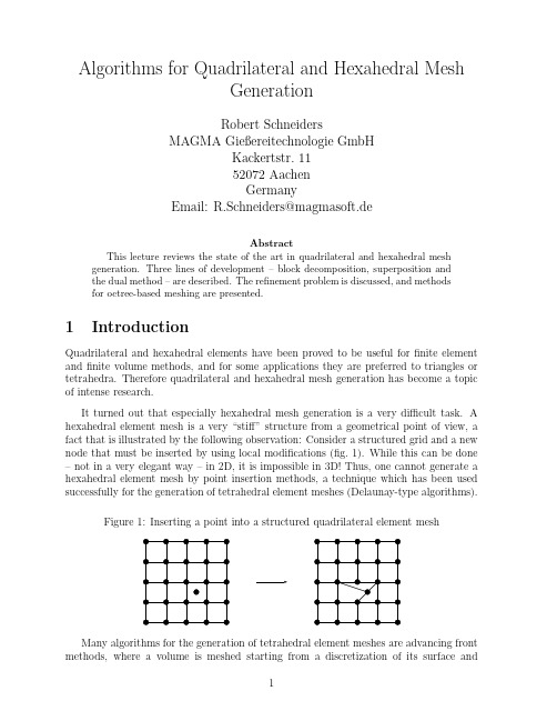
Algorithms for Quadrilateral and Hexahedral MeshGenerationRobert SchneidersMAGMA Gießereitechnologie GmbHKackertstr.1152072AachenGermanyEmail:R.Schneiders@magmasoft.deAbstractThis lecture reviews the state of the art in quadrilateral and hexahedral mesh generation.Three lines of development–block decomposition,superposition andthe dual method–are described.The reﬁnement problem is discussed,and methodsfor octree-based meshing are presented.1IntroductionQuadrilateral and hexahedral elements have been proved to be useful forﬁnite element andﬁnite volume methods,and for some applications they are preferred to triangles or tetrahedra.Therefore quadrilateral and hexahedral mesh generation has become a topic of intense research.It turned out that especially hexahedral mesh generation is a very diﬃcult task.A hexahedral element mesh is a very“stiﬀ”structure from a geometrical point of view,a fact that is illustrated by the following observation:Consider a structured grid and a new node that must be inserted by using local modiﬁcations(ﬁg.1).While this can be done –not in a very elegant way–in2D,it is impossible in3D!Thus,one cannot generate a hexahedral element mesh by point insertion methods,a technique which has been used successfully for the generation of tetrahedral element meshes(Delaunay-type algorithms).Figure1:Inserting a point into a structured quadrilateral element meshMany algorithms for the generation of tetrahedral element meshes are advancing front methods,where a volume is meshed starting from a discretization of its surface and1building the volume mesh layer by layer.It is very diﬃcult to use this idea for hex meshing,even for very simple structures!Fig.2shows a pyramid whose basic square has been split into four and whose triangles have been split into three quadrilateral faces each.It has been shown that a hexahedral element mesh exists whose surface matches the given surface mesh exactly[Mitchell1996],but all known solutions[Carbonera]have degenerated or zero-volume elements.Figure2:Surface mesh for a pyramidThe failure of point-insertion and advancing-front type algorithms severely limits the number of approaches to deal with the hex meshing problem.Most algorithms can be classiﬁed either as block-decomposition,superposition or dual methods,which will be presented in section2,section3and section4.Adaptive mesh generation is more diﬃcult than for triangular and tetrahedral meshes. Fig.3shows an example:The mesh inﬁg.3a has been derived from a structured quadri-lateral mesh by recursively splitting elements.In order to get rid of the hanging nodes, neighboring elements are split to create a conformal transition to the coarse part of the mesh(ﬁg.3b).This probleem is equivalent to the generation of quadrilateral/hexahedral meshes from a quadtree/octree structure.Figure3:Quadrilateral mesh reﬁnementa)b)Fig.4shows a simple example for the3D case(motivated by octree-based meshing) where theﬁne region seems to be connected to the coarse in a reasonable manner.Un-fortunately,the solution is not valid!This can be concluded from the following relation between the number of elements H,the number of internal faces F i and the number of boundary faces F b of a hexahedral mesh:6·H=2·F i+F b(1)Figure4:Non-convex transitioningTherefore,for any hexahedral mesh the number F b of boundary faces must be even. This does not hold for the example ofﬁg.4,so that no hexahedral mesh for that surface mesh exists,and the transitioning is not valid.The mesh reﬁnement problem will be discussed in detail in section5,where we will also solve the problem presented inﬁg.4.Much of the research work has been presented in the Numerical Grid Generation in Computational Fluid Dynamics and in the Mesh Generation Roundtable and Conference conference series,and detailed information can be found in the proceedings.The proceed-ings of the latter one are available online at the Meshing Research Corner[Owen1996], a large database with literature on mesh generation maintained at Carnegie Mellon Uni-versity by S.Owen.Another valuable source of online information is the web page Mesh Generation and Grid Generation on the Web[Schneiders1996d]which provides links to software,literature and homepages of research groups and individuals.An overview on the state of the art in mesh generation is given in the Handbook of Grid Generation [Thompson1999],which has been compiled by the International Society on Grid Gener-ation().2Block-Decomposition MethodsIn the early years of theﬁnite element method,hexahedral element meshes were the meshes of choice.The geometries considered at that time were not very complex(beams, plates),and a hexahedral element mesh could be generated with less eﬀort than a tet mesh(graphics workstations were not available at that time).Meshes were generated by using mapped meshing methods:A mesh deﬁned on the unit cube is transformed onto the desired geometryΩwith the help of a mapping F:[0,1]3→Ω.This method can generate structured grids for cube-like geometries(Fig.5).Figure5:Mapped meshingThe mapping F can be speciﬁed explicitly(isoparametric or conformal mapping)or implicitly(solution of an ellpitic or hyperbolic partial diﬀerential equation).The problem ofﬁnding a suitable mapping F has been the object of major research eﬀorts in recent years,and an overview is given elsewhere in this volume.A summary of the results can be found in the books of Thompson[Thompson1985]and Knupp[Knupp1995].If the geometry to be meshed is too complicated or has reentrant edges,meshes gen-erated by mapped meshing methods usually have poorly-shaped elements and cannot be used for numerical simulations.In this case,a preprocessing step is required:The ge-ometry is interactively partitioned into blocks which are meshed separately(the meshes at joint interfaces must match,a problem considered in[Tam and Armstrong1993]and [M¨u ller-Hannemann1995]).These multiblock-type methods are state of the art in univer-sity and industrial codes.Fig.6shows an example mesh that was generated with Fluent Inc.’s GEOMESH1preprocessor.Figure6:Multiblock-structured meshIn principle,most geometries can be meshed in this way.However,there is a limita-tion in practice:The construction of the multiblock decomposition,which must be done interactively by the engineer.For complex geometries,e.g.aﬂowﬁeld around an airplane or a complicated casting geometry,this task can take weeks or even months to complete. This severely prolongs the simulation turnaround time and limits the acceptance of nu-merical simulations(a recent study suggests that in order to obtain a24-hour simulation turnaround time,the time spent for mesh generation has to be cut to at most one hour).One way to deal with that problem is to develop solvers based on unstructured tetra-hedral element meshes.In the eighties,powerful automatic tethrahedral element meshers have been developed for that purpose(they are described elsewhere in this volume).Theﬁrst attempt to develop a truly automated hex mesher was undertaken by theﬁnite element modeling group at Queens University in Belfast(C.Armstrong).Their strategy is to automate the block decomposition process.The starting point is the derivation of a simpliﬁed geometrical representation of the geometry,the medial axis in2D and the medial surface in3D.In the following we will explain the idea(see [Price,Armstrong,Sabin1995]and[Price and Armstrong1997]for the details).We start with a discussion of the2D algorithm.Consider a domain A for which we want toﬁnd a partition into subdomains A i.We deﬁne the medial axis or skeleton of A as follows:For each point P∈A,the touching circle U r(P)is the largest circle around P which is fully contained in A.The medial axis M(A)is the set of all point P whose touching circles touch the boundaryδA of A more than once.Figure7:Medial axis and domain decompositionThe medial axis consists of nodes and edges and can be viewed as a graph.An example is shown inﬁg.7:Two circles touch the boundary of A exactly twice;the respective midpoints fall on edges of the medial axis.A third circle has three common points with δA,the midpoint is a branch point(node)of the medial axis.The medial axis is a unique description of A:A is the union of all touching circles U r(P),P∈M(A).The medial axis is a representation of the topology of the domain and can thus serve as a starting point for a block decomposition(ﬁg.7and8).For each node of M(A)a subdomain is deﬁned,its boundary consisting of the bisectors of the adja-cent edges and parts ofδA(a modiﬁed procedure is used if non-convex parts ofδA come into play[Price,Armstrong,Sabin1995]).The resulting decompostion of A con-sists of n−polygons,n≥3,whose interior angle are smaller than180o.A polygon is then split up by using the midpoint subdivision technique[Tam and Armstrong1993], [Blacker and Stephenson1991]:It’s centroid is connected to the midpoints of it’s edges, the resulting tesselation consists of convex quadrilaterals.Fig.8shows the multiblock de-compostion and the resulting mesh which can be generated by applying mapped meshing to the faces.It remains to explain how to construct the medial axis.This is done by using a Delaunay technique(ﬁg.9a):The boundaryδA of the domain A is approximated by a polygon p,and the constrained Delaunay triangulation(CDT)of p is computed.One gets an approximation to the medial axis by connection of the circumcircles of the Delaunay triangulation(the approximation is a subset of the Voronoi diagram of p).By reﬁning the discretization p ofδA and applying this procedure one gets a series of approximations that converges to the medial axis(ﬁg.9b).Consider a triangle of the CDT to p:Part of it’s circumcircle overlaps the complement of A.The overlap for theFigure8:Multiblock-decomposition and resulting meshcircumcircle of the respective triangle of the reﬁned polygon’s CDT is signiﬁcantly smaller. If the edge lengths of p tend to zero,the circumcircles converge to circles contained in A which touchδA at least twice.Their midpoints belong to the medial axis.Figure9:Approximating the medial axisa)b)In three dimensions,the automization of the multiblock decomposition is found by using the medial surface.The medial surface is a straightforward generalization of the medial axis and is deﬁned as follows:Consider a point P in the object A and let U r(P) the maximum sphere centered in P that is contained in A.The medial surface is deﬁned as the set of all points P for which U r(P)touches the object boundaryδA more than once.P lies on–a face of the medial surface,if U r(P)touchesδA twice–an edge of the medial surface,if U r(P)touchesδA three times–a node of the medial surface,if U r(P)touchesδA four times or more.The medial surface is a simpliﬁed description of the object(again,A is the union of the touching spheres U r(P)for all points P on the medial surface).The medial surface preserves the topology information and can therefore be used forﬁnding the multiblock decomposition.Armstrong’s algorithm for hexahedral element mesh generation follows the line of the 2D algorithm(ﬁg.10).Theﬁrst step is the construction of the medial surface with the help of a constrained Delaunay triangulation(Shewchuk[Shewchuk1998]shows how to construct a surface triangulation for which a constrained Delaunay triangulation ex-ists).The medial surface is then used to decompose the object into simple subvolumes. This is the crucial step of the algorithm,and it is much more complex than in the two-dimensional case.A number of diﬀerent cases must be considered,especially if non-convexFigure10:Medial-surface algorithm for the generation of hexahedral element meshes(a) medial surface(a) edge primitives(c) vertex primitives(d) face primitives(e) final meshedges are involved;they will not be discussed here,the interested reader is referred to [Price and Armstrong1997]for the details.Figure11:Meshable primitives(selection)Armstrong identiﬁes13polyhedra an object is decomposed to(ﬁg.11shows a selec-tion).These meshable primitives have convex edges,and each node is adjacent to exactly three edges.The midpoint subdivision technique[Tam and Armstrong1993]can there-fore be used to decompose the object into hexahedra:The midpoints of the edges are connected to the midpoints of the faces(ﬁg.12).Then both the edge and face midpoints are connected to the center of the object,and the resulting decompostion consists of valid hexahedral elements.Fig.13shows a mesh generated for a geometry with a non-convex edge.The example highlights the strength of the method:The mesh is well aligned to the geometry,it is a “nice”mesh–an engineer would try to create a mesh like this with an interactive tool.Figure12:Volume decomposition by midpoint subdivision.Figure13:Medial surface and mesh for a mechanical partThe medial surface technique tries to emulate the multiblock decomposition done by the engineer“by hand”.This leads to the generation of quality meshes,but there are some inherent problems:Namely,it does not answer the question whether a good block decomposition exists,which may not be the case if the geometry to be meshed has small features.Another problem is that the medial surface is an unstable entity:Small changes in the object can cause big changes in the medial surface and the generated mesh.Nevertheless,the medial surface is extremly useful for engineering analysis:It can be used for geometry idealization and small feature removal,which simpliﬁes the medial surface,enhances the stability of the algorithm and leads to better block decompositions. The method delivers relatively coarse meshes that are well aligned to the geometry,a highly desirable property especially in computational mechanics.It is natural that an approach to high-quality mesh generation leads to a very complex algorithm,but the problems are likely to be solved.Two other hex meshing algorithms based on the medial surface are known in the litera-ture.Holmes[Holmes1995]uses the medial surface concept to develop meshing templates for simple subvolumes.Chen[Turkkiyah1995]generates a quadrilateral element mesh on the medial surface which is then extended to the volume.3Superposition MethodsThe acronym superposition methods refers to a class of meshing algorithms that use the same basic strategy.All these algorithms start with a mesh that can be more or less easilygenerated and covers a suﬃciently large domain around the object,which is then adapted to the object boundary.The approach is very pragmatic,but the resulting algorithms are very robust,and there are several promising variants.Since we have actively participated in this research,we will concentrate on a descrip-tion of our own work,the grid based algorithm[Schneiders1996a].Fig.14shows the2D variant:A suﬃciently large region around the object is covered by a structured grid.The cell size h of the grid can be chosen arbitrarily,but should be smaller than the smallest feature of the object.It remains to adapt the grid to the object boundary–the most diﬃcult part of the algorithm.Figure14:2D-grid based algorithma)b)c)According to[Schneiders1996a],all elements outside the object or too close to the object boundary are removed from the mesh,with the remaining cells deﬁning the initial mesh(ﬁg.14a,note that the distance between the initial mesh and the boundary is approximately h).The region between the object boundary and the initial mesh is then meshed with the isomorphism technique:The boundary of the initial mesh is a polygon, and for each polygon node,a node on the object boundary is deﬁned(ﬁg.14b).Care must be taken that characteristic points of the object boundary are matched in this step, a problem that is not too diﬃcult to solve in2D.By connecting polygon nodes to their respective nodes on the object boundary,one gets a quadrilateral element mesh in the boundary region(ﬁg.14c).The“principal axis”of the mesh depends on the structure of the initial mesh,and in the grid based algorithm the element layers are parallel to one of the coordinate axis. Consequently,the resulting mesh(ﬁg.14)has a regular structure in the object interior and near boundaries that are parallel to the coordinate axis,irregular nodes can be found in regions close to other parts of the boundary.This is typical for a grid based algorithm, but can be avoided by choosing a diﬀerent type of initial mesh.The only input parameter for the grid based algorithm is the cell size h.In case of failure,it is therefore possible to restart the algorithm with a diﬀerent choice of h,a fact that greatly enhances the robustness of the algorithm.Another way to adapt the initial mesh to the boundary,the projection method,was proposed in[Taghavi1994]and[Ives1995].The starting point is the construction of a structured grid that covers the object(ﬁg.15a),but in contrast to the grid based algorithm,all cells remain in place.Mesh nodes are moved onto the characteristic points of the object and then onto the object edges,so that the object boundary is fully covered by mesh edges(ﬁg.15b).Degenerate elements may be constructed in this step,but disappear after buﬀer layers have been inserted at the object boundary(ﬁg.15c,the mesh is then optimized by Laplacian smoothing).Figure15:Grid based algorithm–boundary adaption by projection techniquea)b)c)The projection method allows the meshing objects with internal faces;the resulting meshes are similar to those generated with the isomorphism techniques,although there tend to be high aspect ratio elements at smaller features of the object.In contrast to the isomorphism technique,the mesh is adapted to the object boundary before inserting the buﬀer layer.Figure16:Grid based algorithm–boundary adaption by cell splitting technique a)b)c)Only recently,a third method has been proposed[Dhondt1999].With this approach,only nodes that are very closed to the bounary are projected onto it.Grid cells that are crossed ty a boundary edge are split(ﬁg.16b).Midpoint subdivision is used to split the 3-and5-noded faces(ﬁg.16c).Dangling nodes are removed by propagating the split throughout the mesh.The superposition principle generalizes for the3D case.The idea of the grid based algorithm is shown for a simple geometry,a pyramid(1quadrilateral,4triangular faces,ﬁg.17).The whole domain is covered with a structured uniform grid with cell size h.In order to adapt the grid to the boundary,all cells outside the object,that intersect the object boundary or are closer the0.5·h to the boundary are removed from the grid.The remaining set of cells is called the initial mesh(ﬁg.17a).Figure17:Initial mesh and isomorphic mesh on the boundarya)b)The isomorphism technique[Schneiders1996a]is used to adapt the initial mesh to the boundary,a step that poses many more problems in3D than in2D.The technique is based on the observation that the boundary of the initial mesh is an unstructured mesh M of quadrilateral elements in3D.An isomorphic mesh M′is generated on the boundary:For each node of v∈M a node v′∈M′is deﬁned on the object boundary,and for each edge (v,w)∈M an edge(v′,w′)∈M′is deﬁned.It follows that for each quadrilateral f∈M of the initial mesh’s surface there is exactly one face f′∈M′on the object boundary. Fig.17b shows the isomorphic mesh for the initial mesh ofﬁg.17b.Fig.18shows the situation in detail:The quadrilateral face(A,B,C,D)∈M cor-responds to the face(a,b,c,d)∈M′.The nodes A,B,C,D,a,b,c,d deﬁne a hexahedral element in the boundary region!This step can be carried out for all pairs of faces,and the boundary region can be meshed with hexahedral elements in this way.The crucial step in the algorithm is the generation of a good quality mesh M′on the object boundary:All object edges must be matched by a sequence of mesh edges, and the shapes of the faces f′∈M′must be non-degenerate.If the surface mesh does not meet these requirements,the resulting volume mesh does not represent the volume well or has degenerate elements.Fulﬁlling this requirement is a non-trivial task,also the implementation becomes a problem(codes based on superposition techniques usually have more than100.000lines of code).We will not describe the process in detail,but some important steps will be discussed for the example shown inﬁgs.19-24.Fig.19a shows the initial mesh for another geometry that does not look very compli-Figure 18:Construction of hexahedral elements in the boundaryregion a bc da’b’c’d’cated but nevertheless is diﬃcult to mesh.The ﬁrst step of the algorithm is to deﬁne thecoordinates of the nodes of the isomorphic mesh.Therefore,normals are deﬁned for thenodes on the surface of the initial mesh by averaging the normals N f of the n adjacentfaces f (cf.ﬁg.19b):N v =1Figure20:Isomorphic surface mesha)b)nodes in space.This allows the optimization of the surface mesh by moving the nodes v′to appropriate positions(ﬁg.20b shows that the quality of the surface mesh can be improved signiﬁcantly).A Laplacian smoothing is applied to the nodes of the surfacemesh:The new position x newi of a node v′is calculated as the average of the midpointsS k of the N adjacent faces.x new i =1from the edge capturing process if three nodes of a face areﬁxed to the same characteristic edge.This cannot be avoided if the object edges are not aligned to the“principal axes”of the mesh(cf.ﬁg.21).There are two ways to deal with the problem.First,the boundary region isﬁlled with a hexahedral element mesh.Due to the meshing procedure,there are two rows of elements adjacent to a convex edge(ﬁg.22a).If the solid angle alongside the edge is suﬃciently smaller than180o,the mesh quality can be improved by inserting an additional row of elements,followed by a local resmoothing. At object vertices where three convex edges meet,one additional element is inserted.Figure22:Inserting additional elements at sharp convex edgesa)b)Fig.24a shows the resulting mesh after the application of the optimization step(note that many degeneracies have been removed).The remaining degenerate elements are removed by a splitting procedure.Figure23:Splitting degenerated elementsa)b)Figure24:Removing degenerated elementsa)b)Fig.23shows the situation:Three points of a face have beenﬁxed to a characteristic edge,the node P is“free”.This face is split up into three quadrilaterals in a way that the ﬂat angle is removed(ﬁg.23b).The adjacent element can be split in a similar way into four hexahedral elements.In order to maintain the conformity of the mesh,the neighborelements must be split up also;it is,however,important that only neighbor elements adjacent to P must be reﬁned,the initial mesh remains unchanged.Fig.24b shows the resulting mesh.Note that the surface mesh is no longer isomorphic to the initial mesh(ﬁg.19a),since removing the degenerated elements has had an eﬀect on the topology(the mesh inﬁg.20b is isomorphic to the initial mesh).The mesh has a regular structure at faces and edges that are parallel to one of the coordinate axes. The mesh is unstructured at edges whose adjacent edges include a“ﬂat”angle and where degenerate elements had to be removed by the splitting operation.Fig.25shows another mesh for a mechanical part.Figure25:Mesh for a mechanical partThe grid based algorithm is only one out of many possible ways use the superposition principle.One can take an arbitrary unstructured hexahedral mesh as a starting point–the adaptation to the boundary is general,no special algorithm is needed.Fig.26shows an example where a non-uniform initial mesh has been generated and adapted to the object boundary by the isomorphism technique.Figure26:Octree-based initial mesh and isomorphic surface meshThis makes the superposition principle a powerful tool for hex meshing.Several vari-ants of the idea have been proposed.Fig.27shows a hexahedral mesh generated to model a part of a turbine.For the smallfeature,a thin initial mesh has been generated.The mesh was adapted to the boundaryby using the method proposed in[Dhondt1999].Figure27:Mesh for a part of a turbineA weak point of the grid based method is the fact that the elements are nearly equal-sized.This can cause problems,since the element size h must be chosen according tothe smallest feature of the object–a mesh with an inacceptable number of elementsmay result.The natural way to overcome this drawback is to choose an octree-basedstructure as an initial mesh.NUMECA’s new unstructured grid generator IGG/Hexa2[Tchon1997]uses this technique,ﬁg.28shows an example of how it works.The initialmesh has hanging nodes,and so does the the mesh on the boundary.Figure28:Fig.29shows a mesh generated with IGG/Hexa around a generic business jet con-ﬁguration.The mesh was generated automatically from an initial cube surrounding thegeometry.Anisotropic adaptation to the geometry is performed in a fully automated waywith a criteria based on normal variation of the surface triangles intersected by the cell.Three layers of high aspect ratio cells are introduced close to the wall.Figure29:Mesh around a jet conﬁgurationThe mesh inﬁg.29has hanging nodes in the interior,which is of disadvantage for some applications.In this case,one can use an octree structure as a starting point,remove thehanging nodes from the octree and use this as an initial mesh.This has been proposed in [Schneiders1998],ﬁg.30shows a shows part of a mesh that has been generated for thesimulation ofﬂow around a car.This technique will be discussed in detail in chapter5ofthis lecture.Figure30:Hexahedral element mesh for the simulation ofﬂow around a carThe grid-and octree-based algorithms presented here prove that the superpositionprinciple is a very useful algorithmic tool to deal with the hex meshing problem.Most commercial hexahedral mesh generators are of this type..The algorithms mentioned here are not the only variants of the strategy,combinations with the other methods seem promising.Further research may reveal the full potential of superposition methods.4The spatial twist continuumThe techniques presented so far can also be used for the generation of tetrahedral ele-ment meshes.In contrast to that,the spatial twist continuum is a unique concept for quadrilateral and hexahedral element mesh generation.Many of the results presented here were achieved by the CUBIT team,a joint re-search group at SANDIA National Laboratories and Brigham Young University that is in quadrilateral and hexahedral element meshing research since the beginning of the 90’s.The group is working on algorithms that generate a mesh starting from discretiza-tion of the object surface into quadrilaterals.As part of their research,the paving [Blacker and Stephenson1991]and plastering[Blacker1993]advancing-front type mesh generators have been developed.These algorithms will be described in chapter6,here we will present other results.Def.1Given an unstructured quadrilateral element mesh M=(V,E,F),the spatial twist continuum(STC)[Murdock et al.1997]M′=(V′,E′,F′)is deﬁned as follows:–For each face f∈F,the midpoint v′is a node of V′.–For each edge e∈E we deﬁne an edge e′=(v′1,v′2)∈E′where v′1and v′2are the midpoints of the two quadrilaterals that share e.For each node v∈V a face f′∈F′is deﬁned by the midpoints of the adjacent quadrilaterals.The STC is the combinatorial dual[Preparata and Shamos1985]of the quadrilateral mesh,just as a Delaunay triangulation and it’s corresponding Voronoi dia-gram are combinatorical dual.Figure31:Quadrilateral mesh and spatial twist continuumFig.31shows a quadrilateral mesh(straight lines)and the STC(dotted lines).The edges of the STC are displayed not as straight lines but as curves.This allows the recognition of chords,a very important structure:One can start at a node,follow an edge e1to the next node,then choose the edge e2“straight ahead”that is not adjacent to e1,continue to the next edge e3and so on.The sequence e1,e2,...forms a chord (displayed as a smooth curve inﬁg.31).Chords can be closed or open curves and can have self-intersections,and no more than2chords are allowed to intersect at one point.。

AM_12_Chapter 6_Sweep Meshing

6-9
Sweep Meshing
Sweepable Bodies
• A body is sweepable if:
ANSYS, Inc. Proprietary © 2009 ANSYS, Inc. All rights reserved.
6-7
April 28, 2009 Inventory #002645
Sweep Meshing
Comparing Workbench Sweep Methods
Training Manual
Thin Sweep Method:
• Sweeps multiple sources to paired multiple targets • Good substitute for midsurfacing shell models to get a pure hex mesh
Sweep Method:
There are 3 hex meshing or sweeping approaches in Workbench ANSYS Meshing: 1. Sweep Method
• Traditional sweep p method • Improved at R12
Training Manual
ANSYS, Inc. Proprietary © 2009 ANSYS, Inc. All rights reserved.
6-5
April 28, 2009 Inventory #002645
Sweep Meshing
Challenges with Sweeping
•
Training Manual
• Sweeps a single source/face to a single target/face. • Does a good job of handling multiple side faces along sweep • Geometry needs to be decomposed so that each sweep path is represented by 1 body.

新的点云数据精简存储方法

新的点云数据精简存储方法张有亮;刘建永;付成群;郭杰【摘要】海量点云数据的精简存储是逆向建模的一个关键环节,针对单站地面固定式三维激光扫描点云扇形等特点,提出了一种新的点云精简存储方法——扇形网格法.对点云数据遍历一次,即完成对点云的精简、降噪与存储,并用VC++6.0编写实现.多站扫描点云的配准、拼接,如果在单站点云经过扇形网格法处理后进行,会更快速高效.在与传统点云压缩算法分析对比的基础上,对其特点进行了分析,对在战场地形数字化中的适用性进行了验证.%The reduction and storage of enormous point cloud data is a crucial link in reverse modelreconstruction.Considering the features of point cloud data by single station laser scanning, a new method — grid sector method was put forward for its reduction and storage. Point cloud data could be filtered and stored only by traversal. This method was realized on VC ++6.0. Multi-station scanning of point cloud registration and stitching would be more quickly and efficiently, if the site goes through the fan in a single grid after treatment. Based on the contrast with traditional compressing methods, this paper analyzed its characteristics and proved its applicability in battlefield terrain digitization.【期刊名称】《计算机应用》【年(卷),期】2011(031)005【总页数】3页(P1255-1257)【关键词】单站三维激光扫描;点云数据;精简存储;扇形网格法;战场地形数字化【作者】张有亮;刘建永;付成群;郭杰【作者单位】解放军理工大学工程兵工程学院,南京210007;解放军理工大学工程兵工程学院,南京210007;解放军理工大学工程兵工程学院,南京210007;解放军理工大学工程兵工程学院,南京210007【正文语种】中文【中图分类】TP751.1;TP391.750 引言海量点云数据的精简存储是逆向建模的一个关键环节，目前国内外学者在点云数据的精简压缩算法上做了大量的工作。

Autodesk IPG Reality Computing教程：从照片到3D说明书

From Real to Digital and back to PhysicalMitko Vidanovski – Product Specialist - Autodesk IPG Reality ComputingTatjana Dzambazova – Sr.Product Manager - Autodesk IPG Reality ComputingDeepak Maini –Technical Head - Manufacturing SolutionsClass ID RC3345-LFrom photos to 3D — this hands-on lab will teach you how it is really done. We’ll cover best practices for taking photos for photogrammetry in various types of environments. We will then get a deep dive in Autodesk® ReCap™ Photo, covering basic photo reconstruction, as well as manual stitch and survey points. From there, we will proceed to model preparation and postproduction in in Project Memento and Meshmixer 2.0 that are necessary for preparing high-quality meshes for digital output and fabrication. We’ll also cover the basic for creating high quality visualization in form of turntable and animation of the final results in Maya.Learning ObjectivesAt the end of this class, you will be able to:•Take best possible photos for photogrammetry•Convert Photos into 3D models;•3D print models created from Photos;•Laser cut or CNC your models from Photos;•Create an animation, turntable and basic renderings;•Attain advanced modeling techniques;About the SpeakerMitko Vidanovski is a technologist with a Master Degree in Architecture. From the early days of his studies, he was intrigued by digital design technology, and he began exploring a number of CAD, 3D modeling, rendering and animation tools which he soon mastered.In 2012 he joined Autodesk’s Reality Computing group, and soon to become the technical expert of the group. He is responsible for making pilot tests of new technologies involving 3D laser scanning and photogrammetry, conducting training and creating a technical marketing collateral.Previous to Autodesk, Mitko worked in progressive environments such as Otherlab and Because We Can, where he gained experience in various fabrication technologies, such as 3D printing, laser cutting and CNC milling.1.Best photo capture practiceso For Interior scenes;o For Exterior scenes;o For sculptures and objects;o Aerial photogrammetry;o Underwater photogrammetry;o Various capture devices (DSLR, cell phones, GoPro)o Best camera capture settings;o Images post processing tips;(Explanation)232. Best use of ReCap Photo on ReCap 360o Which photos to use;o Adopt to specific scenario;o Use of survey points and measurements on ReCap 360;o Match your ReCap Photo reconstruction with existing model or laser scan; oHow to combine two or more reconstructions into one;(Explanation)43. Clean and prepare your 3D models in Project Mementoo Import OBJ, or open an RCM file; o Clean up the scene;o Cut & fill the base of an object; o Check you model for errors; oDecimate and export;(Hands-on)54. Advanced modeling techniques in Meshmixer 2.0o Import textured model in Meshmixer; o Fix bad areas with the model; o Smooth and optimize;o Properly orientate your model; o Use of Slice tool; o Measure and scale; o Create a base;oMake your models hollow and add thickness;(Hands-on)65. The basics for creating renders and animation in Mayao Import and set-up your model;o Tweak preferences and render settings; o Import and set-up camera;o Setting up key frames and work with the timetable; oRender;(Hands-on)。

Ansys workbench Mech-Intro_14.0_L04_Meshing网格划分-中英文对照

Release 14.0
… Global Meshing Controls
Shape Checking:
整体网格划分控制
Again some of the advanced mesh settings are beyond the scope of the introductory course (or apply to other physics). Several controls have potential application in linear static analysis. 再一次强调，一些高级网格设置超出了培训课程的范围（或适用于
概要
In this chapter controlling meshing operations is described.
这一章，我们将介绍与网络划分相关的操作。 Topics: A.整体网格控制 A. Global Meshing Controls B. Local Meshing Controls B.局部网格控制 C. Meshing Troubleshooting C.网格划分故障诊断 D. Virtual Topology D.虚拟拓扑 E.workshop 4-1，“网格控制” E. Workshop 4-1, “Meshing Control”
Release 14.0
… Global Meshing Controls
整体网格划分控制
Proximity provides a means to control the mesh density in regions of the model where features are located closer together. In cases where the geometry contains lots of detail this can be a quick way to refine the mesh in all areas without applying numerous local controls. "Proximity" 可以用来调整模型的网格密度，其中这些模型的特征相近。它 As mentioned earlier proximity and curvature can be combined. The choice of control is dictated by the geometry being meshed.

数字图像处理-冈萨雷斯-课件(英文)Chapter03 空域图像增强

Power-Law Transformations : Gamma Correction Application Ariel images after Gamma Correction
(Images from Rafael C. Gonzalez and Richard E. Wood, Digital Image Processing, 2nd Edition.
Desired image
Image displayed at Monitor
After
Gamma correction
Image displayed at Monitor
(Images from Rafael C. Gonzalez and Richard E. Wood, Digital Image Processing, 2nd Edition.
Ds
Dr Smaller Dr yields wider Ds = increasing Contrast
(Images from Rafael C. Gonzalez and Richard E. Wood, Digital Image Processing, 2nd Edition.
Gray Level Slicing
(Images from Rafael C. Gonzalez and Richard E. Wood, Digital Image Processing, 2nd Edition.
Histogram of an Image (cont.)
low contrast image has narrow histogram
high contrast image has wide histogram

纹理物体缺陷的视觉检测算法研究--优秀毕业论文

摘要
在竞争激烈的工业自动化生产过程中，机器视觉对产品质量的把关起着举足轻重的作用，机器视觉在缺陷检测技术方面的应用也逐渐普遍起来。与常规的检测技术相比，自动化的视觉检测系统更加经济、快捷、高效与安全。纹理物体在工业生产中广泛存在，像用于半导体装配和封装底板和发光二极管，现代化电子系统中的印制电路板，以及纺织行业中的布匹和织物等都可认为是含有纹理特征的物体。本论文主要致力于纹理物体的缺陷检测技术研究，为纹理物体的自动化检测提供高效而可靠的检测算法。纹理是描述图像内容的重要特征，纹理分析也已经被成功的应用与纹理分割和纹理分类当中。本研究提出了一种基于纹理分析技术和参考比较方式的缺陷检测算法。这种算法能容忍物体变形引起的图像配准误差，对纹理的影响也具有鲁棒性。本算法旨在为检测出的缺陷区域提供丰富而重要的物理意义，如缺陷区域的大小、形状、亮度对比度及空间分布等。同时，在参考图像可行的情况下，本算法可用于同质纹理物体和非同质纹理物体的检测，对非纹理物体的检测也可取得不错的效果。在整个检测过程中，我们采用了可调控金字塔的纹理分析和重构技术。与传统的小波纹理分析技术不同，我们在小波域中加入处理物体变形和纹理影响的容忍度控制算法，来实现容忍物体变形和对纹理影响鲁棒的目的。最后可调控金字塔的重构保证了缺陷区域物理意义恢复的准确性。实验阶段，我们检测了一系列具有实际应用价值的图像。实验结果表明本文提出的纹理物体缺陷检测算法具有高效性和易于实现性。关键字: 缺陷检测；纹理；物体变形；可调控金字塔；重构
Keywords: defect detection, texture, object distortion, steerable pyramid, reconstruction
II

1、下载文档前请自行甄别文档内容的完整性，平台不提供额外的编辑、内容补充、找答案等附加服务。
2、"仅部分预览"的文档,不可在线预览部分如存在完整性等问题,可反馈申请退款(可完整预览的文档不适用该条件!)。
3、如文档侵犯您的权益，请联系客服反馈,我们会尽快为您处理(人工客服工作时间：9:00-18:30)。

Extending Progressive Meshes for Use over UnreliableNetworksZhihua Chen Dept.of Electrical Engineering and Computer ScienceVanderbilt UniversityNashville,TN37235zhihua.chen@Bobby BodenheimerDept.of Electrical Engineeringand Computer ScienceVanderbilt UniversityNashville,TN37235bobbyb@J.Fritz BarnesDept.of Electrical Engineeringand Computer ScienceVanderbilt UniversityNashville,TN37235J.Fritz.Barnes@ABSTRACTProgressive meshes[7]provide an attractive mechanism for trans-mitting3D geometry over networks.Progressive meshes(PM) transmit a coarse initial mesh and reﬁnements that can be applied to the initial mesh.However,these techniques assume a reliable network protocol such as TCP/IP is used for data transmission. When transmitting3D geometry for graphical applications such as concurrent virtual environments distributed over wide area net-works with some nodes potentially using wireless networks,many losses will occur.TCP/IP performance degrades in the presence of packet loss and multicast communication mechanisms typically do not provide reliable communication.These applications motivate the issue of transmitting geometric data over unreliable networks. In this paper,we discuss several errors that are caused when re-constructing PM geometries after some packets have been lost.We modify the PM data structures to improve robustness during packet loss.We use these modiﬁcations to improve a hybrid transmission technique that uses TCP to transmit the base mesh and portion of the initial mesh and then use UDP to transmit the remainder of the mesh to improve transmission performance.1.INTRODUCTIONAs the Internet expands,demand is growing for high quality 3D geometry in applications,from games such as Everquest[5]to collaborative virtual environments to multimedia and purely web-based applications.Such applications use high resolution3D meshes to achieve their effect,and the challenge of the growing demand for these meshes is how to store and transmit the large amount of data contained in them.Hoppe[7]proposed the progressive mesh(PM)technique as an initial solution for the transmission of geometric data over data net-works.In this method,the server initially sends coarse shape in-formation to a client that can be reconstructed and rendered very quickly.Then increasing detail in the model is transmitted to the client,allowing the client to progressively reﬁne the initial model into the full resolution model.Various authors,e.g.,[10]and others,have combined mesh com-pression techniques with progressive transmission to reduce the amount of data that needs to be sent.Typically,there is a trade-off between compression ratio and the fragility of the compressed mesh.In prior work,we demonstrated that using an unreliable channel can improve transmission times by as much as forty per-cent with a negligible drop in visual quality[4].In this work,we in-vestigate mechanisms that extend the PM technique to handle ran-dom losses occurring in the transmission channel.We describe the ﬂaws that occur when packets are lost using the PM technique and modiﬁcations and heuristics that can be used to improve the visual quality of models when some packets have been lost.These mod-iﬁcations allow additional improvements in the transmission time over unreliable networks.The paper is organized in the following manner.In Section2 we place our work in context of what has been done in this area. Section3details the modiﬁcations to the basic PM scheme needed when data loss can occur.Section4discusses our hybrid transmis-sion protocol.Section5presents the results of actual transmission experiments over a lossy network with an analysis of them.Finally, in Section6we discuss our results.2.OUR WORK IN CONTEXTThe PM scheme was devised by Hoppe in[7,9],and we have implemented the basic versions without the modiﬁcations of later work,e.g.,[8].The reader is referred to thos papers for a detailed discussion;here we simply present enough information to famil-iarize the reader with our notation.The PM representation of a mesh is stored as a coarse mesh and a sequence of de-tail records called vertex splits.These vertex splits indicate how to incrementally reﬁne so that after the vertex splits have been processed,the original mesh is recovered.In fact,the PM rep-resentation deﬁnes a sequence of meshes which provide increasingly accurate approximations of.A vertex split is a basic transformation that adds a vertex to the mesh.The basic progressive mesh scheme is implemented, but for the purposes of this paper,a vertex split does not contain normal,texture,or material information.Each vertex split is a30 byte quantity consisting of a face index,,an index(),an encoding,and two vertex position deltas,and.In our experiments,these vertex splits are packed into1400byte packets.Thus,each packet contains roughly 46vertex splits.Figure1illustrates a PM vertex split transformation.Each ver-tex split operation introduces a new vertex and two new faces, as shown.The location of a vertex split is parameterized by,, and.By default,the PM data structure does not include inci-dence information in the vertex to face direction.The vertex values are determined through theﬁelds,,and. To determine the vertex being split(),the three vertices of the face are sorted by their index values and stored into an or-dered list.They are indexed by.Vertex is the next vertex clockwise on the face.The vertex is determined by,the number of clockwise rotations about from to .Other techniques for mesh decomposition with an idea towardsFigure1:Vertex splittransformation.Figure2:The Buddha model after transmission over a lossynetwork:(a)no change to PM data structures;(b)using ab-solute;(c)using both absolute and alteredﬁeld.robust transmission exist,e.g.[3,10,1].Most of these techniqueshave not been tested in as rigorous an environment as our methods.In the context of progressive transmission,much of the work hasfocused on better methods of transmission,e.g.,[10,2,6].Thesetechniques are complementary to our own,in that they couldﬁtwithin the techniques proposed here to achieve higher transmissionrates.3.MODIFICATIONS TO THE PM DATASTRUCTUREWhen the transmission channel is lossy,vertex splits will be(a)(b)f==ff20f45966565ff114Figure3:Illustration of self-intersection occurrence caused by:(a)No packet loss,intermediate vertex splits changethe three vertices of face to65,96and114;(b)Packets con-taining the intermediate vertex splits are lost,the three verticesof face remain unchanged as65,20,45.=4(a)=4(b)Figure4:Illustration of self-intersection occurrence caused by:(a)No packet loss,intermediate vertex splits changethe number of faces around to8;(b)Packets containing theintermediate vertex splits are lost,the number of faces aroundremain unchanged at6.lost when packets are lost.As a result,the geometry of the re-constructed model can be corrupted.This corruption most oftentakes the form of surface self-intersection,i.e.,parts of the surfaceintersecting with the surface itself.The self-intersections destroythe manifold property that the surfaces in the original model haveand create visual artifacts in the reconstructed models,as shownin Figure2(a).In this section we discuss how lost vertex splitscause self-intersections to occur and describe modiﬁcations to thePM data structure that improve the situation.First,in addition to a packet containing only vertex split infor-mation,each packet contains a4byte header that stores the indexnumber of theﬁrst face of the mesh that will be introduced by theﬁrst vertex split in this packet.The client renderer uses this num-ber as a“poor man’s”error correction,to give faces generated byvertex splits after lost packets their index number in the full reso-lution mesh.This process is done so that future splits whose faceindex,,reference these faces will be able toﬁnd them.Thisheader is a monotonically increasing number,and can also be usedto detect out-of-order packets.One cause of self-intersection is that theﬁeld in a ver-tex split record is the numerical order of the index valueof the split vertex among the three vertices on(see Fig-ure1).When vertex splits are lost,the index values of the verticeson may become different from what they were when the pro-gressive mesh was generated.Thus,the ordering of the verticesmay be wrong.This change of ordering causes the PM reconstruc-tion toﬁnd the wrong,which results in geometric corruption.For example,in Figure3(a),without packet loss,intermediate ver-tex splits change the three vertices of face to65,96and114.A subsequent vertex split with=66and=1splitsvertex96because its index is the second smallest.When the inter-mediate splits are lost,as shown in Figure3(b),the three verticesof face remain unchanged as65,20,45.Now vertex45has thesecond smallest index among the vertices of.The same splitwith=66and=1then splits vertex45and causesthe faces connected with the added vertex to pierce the top rightface.The PM data does not store how the three vertices of a face tobe reconstructed were ordered in the vertex list of the face in theoriginal model.Therefore,the ordering of vertices in the vertexlist of a face in the reconstructed model may be different fromthat in the original model.This fact is part of the reason why thewas deﬁned as a order of index value ratherthan the placement of in the vertex list of.Toalleviate this problem,we add a second pass over the PM data toreplace each with the placement ofat the time of the vertex split.The time the second pass takesis negligible compared with the time to generate the progressive meshes.When this change is incorporated a signiﬁcant number ofself-intersections can be eliminated,as shown in Figure2(b).Theﬁeld in a vertex split record can also cause self-intersections to occur.Theﬁeld,as originally deﬁned,isthe number of clockwise rotations from to about.Whenvertex splits are lost,the number of rotations from to may be different from what it was in its original context,or may notexist at all.This difference can cause the reconstruction programto pick the wrong,resulting in geometric corruption as shownin Figure4.To help the reconstruction program detect this casewithout changing the size of the PM data structure,we modify the ﬁeld.Instead of using16bits for theﬁeld,we use8bits,and use the remaining8bits to encode a quantity called .Theﬁeld stores the total number of faces around.The reconstruction program checks the atrun time and discards splits whose do not match thosein the partially reconstructed meshes.When this change is incor-porated,additional self-intersections can be eliminated,as shown in Figure2(c).4.HYBRID TRANSMISSIONThe progressive mesh format creates an alternative representa-tion of the3D geometry.One signiﬁcant advantage of this repre-sentation is that some packets containing mesh data are more im-portant than other packets.In particular,initial splits provide sig-niﬁcant improvements as measured by the Hausdorff metric,while later splits provide decreasing beneﬁts.Our hybrid technique leverages the inherent differences that ver-tex splits have on the resulting visual accuracy of the reconstructed mesh.Thus,in this scheme,we begin by transmitting data using the TCP protocol.Part-way through the transmission,the hybrid sender closes the TCP connection and transmits the remaining data using UDP.Details on these protocols can be found in[4].This technique allows the sender to reliably transfer the base mesh and some of the initial splits and use a more aggressive technique to transfer less important splits.TCP controls the rate that packets are sent to maintainﬂow con-trol and minimize congestion.As a result,TCP does not provide the end-user control of the sending rate.When we consider using UDP for transmission of data,the end-user has signiﬁcant inﬂuence over the send rate.Therefore,our application must carefully select the send rate.If the send rate exceeds the capacity of the channel, we will increase the number of packets lost.However,if we de-crease the send rate,we will not lose any packets but the transfer of information will take much longer than a TCP connection might take.We experimentally determine UDP send rates to use in appli-cations.In future work,we will investigate automatic mechanisms for setting the UDP send rate.An issue of concern in implementing this idea is that the sender can begin sending UDP data to the receiver while the receiver is still reading data from the TCP connection.This behavior causes a problem since the initial data willﬁll up the operating system’s buffer for incoming network data and start dropping UDP pack-ets that arrive.Therefore,the hybrid protocol adds a delay before sending the UDP data until the receiver has received all TCP data.5.EXPERIMENTAL RESULTSWe tested our transmission methods by running a set of exper-iments with varying levels of background load using a variety of models.The experimental setup is identical to that described in[4]; for reasons of space,the reader is referred there for details.Also forFigure5:The average time of transmission of the Buddha model versus the channel capacity for the different transmis-sion schemes(TCP/UDP ratios).The UDP send rate was11.424 Mbps.reasons of space,we report results for only one model,the“happy Buddha”model.The Buddha model contains1.08M faces in its full model and1998faces in its base mesh.The suite of experi-ments was run using different send rates for the UDP portion of the model transmission.5.1Results for Buddha ModelOur extensions to the PM data structure cause additional splits to be rejected because they cause geometric corruption,as discussed earlier.Theﬁrst modiﬁcation generally does not cause much im-pact on the total number of faces reconstructed.For example,over ten trials using the Buddha model,transmitting25%of the data with TCP in addition to the base mesh causes less than1%of the splits to be rejected(893k faces reconstructed on average versus 889k faces with the absolute index modiﬁcation in place).The second modiﬁcation,changing theﬁeld,is more severe, and on average causes24%of the splits to be rejected over the method without modiﬁcation(679k faces reconstructed on average with both modiﬁcations in place).Nonetheless,we believe the im-provement in visual quality justiﬁes the changes.Figure5shows the average transmission time for the various transmission schemes,and Figure6shows the average number of faces received versus channel capacity.In theseﬁgures,the UDP send rate was11.424Mbps,and TCP was used to transmit the base mesh plus0to50%of the rest of the model.The important result in Figure5is that the transmission time to send the model using pure TCP is the longest.Moreover,as the ratio of packets sent by TCP decreases,the transmission time improves for all given levels of noise.To explain this behavior,one must consider what happens when we increase the amount of noise.When the noise exceeds the channel capacity,the channel is full,and buffers in the network become saturated.This saturation results in packet loss.Packet loss causes TCP to incur timeouts or apply the fast retransmission scheme.Thus,the transmission time using TCP increases.As a ﬁnal note,the0%TCP plot in thisﬁgure is not quite constant be-cause,as mentioned,the base mesh is transmitted reliably using TCP.This transmission time improvement comes at a cost,however. Figure6shows the number of faces in the received model for each of these transmission methods.Note that TCP,since it is a reliable transport protocol,always transmits all the faces.When a portion of the packets are sent using UDP,signiﬁcant packet loss can oc-cur,and this loss becomes worse as the noise increases.There-fore the selection of an appropriate hybrid protocol will depend on the tradeoff between the transmission time and the visual degrada-tion that occurs when packets are lost.The visual degradation of this process is shown in the Buddha model in Figure7.Thisﬁg-Figure 6:The number of faces received of the Buddha model versus channel capacity for the different transmission schemes (TCP/UDP ratios).The UDP send rate was 11.424Mbps.Figure 7:The Buddha model after transmission over a lossy network:(a)the full model as sent by TCP;(b)model received when 50%transmitted by TCP;(c)model when 25%sent by TCP;(d)model when 12.5%sent by TCP;(e)model when fully sent via UDP.ure shows the models that were received in one experiment using a UDP send rate of 11.424Mbps and where the noise consumed 109%of the channel capacity.In particular,the visual quality of the model is excellent when 12.5%of it is transmitted via TCP.TCP took on average 131seconds to transmit at this noise level,while the average transmission time for the 12.5%scheme was 27seconds,a considerable savings.A signiﬁcant concern in any transmission scheme is that the band-width of the scheme is minimal.In Figure 8,we compare the num-ber of bytes used to transmit the Buddha model by both TCP and UDP as we increase the amount of background noise.UDP is con-stant by design—it is equivalent to the TCP 0%line in the previous ﬁgures.Note that TCP uses more bandwidth as the noise increases,from 1.3to 4.6%.This result is unsurprising since TCP must re-send lost packets,requires the use of acknowledgments,and has a larger header size than UDP packets.Note that the comparison in Figure 8does not include the bandwidth of packets used to ac-knowledge receipt of data by the PM receiver.6.CONCLUSIONIn this paper,we have modiﬁed the progressive mesh data struc-ture to enable it to more robustly transmit 3D geometric data over lossy channels.We demonstrated this modiﬁcation in the context of a hybridtransmission scheme,and showed that the hybrid ap-proach improves the transmission performance.This improvement in performance comes at the cost of lost packets.The progressive mesh representation allows us to minimize the visual impact when packets are lost,although some surface corruption is visible.The visual results indicate that geometric corruption has minimal im-pact on the visual quality of the mesh.Figure 8:Total bytes sent by TCP (dashed line)and UDP (solid line)versus noise in the channel.Note that the UDP send rate is constant,but the number of bytes sent by TCP increases as it must resend data due to lost packets.We are currently investigating methods of representing and re-constructing the progressive mesh that eliminate this corruption with less overhead than employing a forward error correction (FEC)code arbitrarily on the data.REFERENCES[1]A L -R EGIB ,G.,AND A LTUNBASAK ,Y.An unequal errorprotection method for packet loss resilient 3-d meshtransmission.In Proceedings of INFOCOM 2002(2002).[2]A LLIEZ ,P.,AND D ESBRUN ,M.Progressive compressionfor lossless transmission of triangle meshes.In Proceedings of ACM SIGGRAPH 2001(July 2001),Computer Graphics Proceedings,Annual Conference Series,ACM Press /ACM SIGGRAPH /Addison Wesley Longman,pp.195–202.[3]B ISCHOFF ,S.,AND K OBBELT ,L.Streaming 3d geometryover lossy communication channels.In Proceedings of the IEEE International Conference on Multimedia and Expo (2002).[4]C HEN ,Z.,B ODENHEIMER ,B.,AND B ARNES ,J.F.Robusttransmission of 3d geometry over lossy networks.In Web3D 2003Symposium Proceedings (St.Malo,France,Mar.2003),ACM SIGGRAPH,pp.161–172.[5]E VERQUEST ..[6]G ANDOIN ,P.-M.,AND D EVILLERS ,O.Progressivelossless compression of arbitrary simplicial complexes.ACM Transactions on Graphics 21,3(July 2002),372–379.ISSN 0730-0301(Proceedings of ACM SIGGRAPH 2002).[7]H OPPE ,H.Progressive meshes.In Proceedings ofSIGGRAPH 96(New Orleans,Louisiana,August 1996),Computer Graphics Proceedings,Annual Conference Series,ACM SIGGRAPH /Addison Wesley,pp.99–108.ISBN 0-201-94800-1.[8]H OPPE ,H.View-dependent reﬁnement of progressivemeshes.In Proceedings of SIGGRAPH 97(Los Angeles,California,August 1997),Computer Graphics Proceedings,Annual Conference Series,ACM SIGGRAPH /Addison Wesley,p.I198.ISBN 0-89791-896-7.[9]H OPPE ,H.Efﬁcient implementation of progressive meshes.Computers &Graphics 22,1(February 1998),27–36.ISSN 0097-8493.[10]P AJAROLA ,R.,AND R OSSIGNAC ,pressedprogressive meshes.IEEE Transactions on Visualization and Computer Graphics 6,1(January -March 2000),79–93.ISSN 1077-2626.。