Autolab中文操作手册
Autolab 电位器和 NOVA 控制器程序的电化学测量说明书
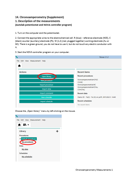
14. Chronoamperometry (Supplement)1. Description of the measurements(Autolab potentiostat and NOVA controller program)1. Turn on the computer and the potentiostat.2. Connect the appropriate wires to the electrochemical cell. R (blue) - reference electrode (NCE), C (black) counter (auxiliary) electrode (Pt), W (1,2) (red, plugged together) working electrode (Au or GC). There is a green ground, you do not have to use it, but do not touch any electric conductor with it.3. Start the NOVA controller program on your computer.Choose the …Open library” menu by left-clicking on the mouse.Clicking on the …My procedures” menu, you could find the procedures (programs) used in the measurements.Choose the appropriate procedure to what you want to do. Read the …Remarks” field also to choose the right program.For Chronoamperometric measurements, the parameters given in the measurement description are already set. The procedure looks like this.Each icon indicates "Commands", which makes the measurement happen. The first icon, "Autolab control" is used to detect the measuring instrument, to set the potentiostatic mode, and to select the current range. The second icon, "Apply", sets the initial electrode potential at the input of the potentiostat. The third icon, "Cell on", connects the potentiostat to the electrochemical cell. The fourth icon, "Wait", keeps the working electrode for the specified time at the initial potential. The fifth icon, "Apply", indicates the potential step to the specified value. The sixth icon, "Record signals", performs the measurement of the time depending current after the potential step. The seventh icon, "Cell Off" turns the cell off from the potentiostat, finishes the measurement. The measurement procedure and the measured data are automatically saved in a .nox file that can be found later on the "My data" menu in the "Library" menu. The data file name is the file name of the "Procedure" plus a "Timestamp", i.e. when the measurement was made. Therefore, it is important to note the order of measurements so that their results can easily be found later.The measurement can be started by clicking on the "Run" command in the "Measurement" menu on the top of the screen or by clicking the Play ( ) icon above the Procedure.During the measurement, instead of the Play icon, the Pause ( ) and Stop ( ) icons will be displayed. If you notice a problem, stop the measurement.During the measurement, the computer automatically plots the measured data in the Plots window in the lower left corner of the screen.Physically, the data files are stored in the Dokumentumok Library in the NOVA 2.1 folder in the Data subfolder. From there, you can make a copy, e.g. to a pendrive.…Behind” each Command icon you could find "Subcommands", shown on the right side of the Procedure pane, or you can see the details with the "More" command by clicking on the corresponding icon. If it is possible, do not change the parameters, or if this happened, DO NOT SAVE THE ALTERED PROCEDURE WITH ITS ORIGINAL NAME.For cyclic voltammetric measurements, the "Procedure" looks like this:Each icon indicates "Commands", which makes the measurement happen. The first icon, "Autolab control" (Autolab control) is used to detect the measuring instrument, to set the potentiostatic mode, and to select the current range. The second icon, "Message", asks for the applicable scan rate ("Scan rate (V/s)"). Once the measurement is started, it must be set to the desired value. The third icon, "Apply", sets the initial electrode potential at the input of the potentiostat. The fourth icon, "Cell on", switches the potentiostat to the electrochemical cell. The fifth icon, "Wait", keeps the working electrode for the specified time at the initial potential. The sixth icon, "CV staircase", represents the cyclic measurement between the lower and upper potential limits with the scan rate given in the …Message". The seventh icon, "Cell Off" turns the cell off from the potentiostat, finishes the measurement. The measurement procedure and the measured data are automatically saved in a .nox file that can be found later on the "My data" menu in the "Library" menu. The data file name is the file name of the "Procedure" plus a "Timestamp", i.e. when the measurement was made. Therefore, it is important to note the order of measurements so that their results can easily be found later.The measurement can be started by clicking on the "Run" command in the "Measurement" menu on the top of the screen or by clicking the Play ( ) icon above the Procedure.During the measurement, instead of the Play icon, the Pause ( ) and Stop ( ) icons will be displayed. If you notice a problem, stop the measurement.During the measurement, the computer automatically plots the measured data in the Plots window in the lower left corner of the screen.Physically, the data files are stored in the Dokumentumok Library in the NOVA 2.1 folder in the Data subfolder. From there, you can make a copy, e.g. to a pendrive.…Behind” each Command icon you could find "Subcommands", shown on the right side of the Procedure pane, or you can see the details with the "More" command by clicking on the corresponding icon. If it is possible, do not change the parameters, or if this happened, DO NOT SAVE THE ALTERED PROCEDURE WITH ITS ORIGINAL NAME.The only parameter you have to set is "Scan rate (V/s)". For sequential runs, use the order that is described in the measurement description. (For example HCF solutions 0.320 V/s, 0.160 V/s, 0.080V/s, etc.)IMPORTANT! NOVA uses Windows default decimal separator. See that the "Message" contains the default value, and that the entered value is also correct! (For example, 0,08 or 0.08!) The data exported from the NOVA also uses the same decimal separator. If necessary, change it to the settings in the Excel Options menu in accordance with the Windows setup!2. Description of evaluation(Autolab potentiometer and NOVA controller program)The NOVA software used for the measurements can be applied for many purposes, but the User's manual is 1196 pages, which is a bit tiring in a lab to read. Therefore, only the most important functions are highlighted.For the evaluation of voltammograms, it is necessary to determine the peak potentials (E p), half peak current potentials (E p/2) and the background corrected peak currents (I p). This can be done in Excel after exporting the measurement data. To do this, double-click the "Plots" pane.Instead of the procedure, the measured plot is displayed in the main window.Clicking on the …Show data” icon you could see a table.In the top right corner there is a marker leading to the export function.Select Excel Export from "File Format", and Windows Explorer will save the file to the desired name and location.ATTENTION! The Excel file contains only the measured data (maybe calculated data, as well), not the description of the Procedure! It's still in the .nox files, do not delete them.IMPORTANT! NOVA uses Windows default decimal separator. The data exported from the NOVA also uses the same decimal separator. If necessary, change it to the settings in the Excel Options menu in accordance with the Windows setup!For Excel files, you can get the desired data, graphics, where needed.For the evaluation of voltammograms, it is necessary to determine the peak potentials (E p), half peak current potentials (E p/2) and the background corrected peak currents (I p). This can be done in Excel after exporting the measurement data, but (perhaps) simpler in NOVA with an "Analysis" function.Click the microscope icon to see a menu. Select "Peak search" analysis.Then, a submenu "Properties" opens in the right window, which offers different versions of the peak search. The default setting is "Automatic", and the figure (or the table) also shows this result, but this is usually good for nothing!Select "Manual", and "Linear free cursor" option.Returning to the plot in the main window with the mouse, you could see a cross. Set this to the initial part of the voltammogram, and fix it with a click. Drag a straight line with the mouse that best fits thefirst part of the voltammogram. The end of the line does not have to be on the curve (free cursor). You can fix the straight line with another click, and the results of the peak search appear in the "Properties" window on the right. (Another voltammogram is illustrated because there will be many peaks on the earlier example.)The same can also be done for the cathodic peak, however from the other end of the curve, the straight line must be fitted backwards.All of these can go in succession, the peaks are included in the right table ("Peaks"). If you are not satisfied with the fitting, you can resume the search at any time by pressing the "Reset" button.The values in the table are:1 Number of found peaks"Peak position" is the electrode potential of the found peak in Volt"Peak height" is the corrected value of the peak current in Amper"Peak (1/2)" is the difference between the potential at the peak current and the potential at the half peak current, i.e. Peak (1/2) = E p– E P/2. (Signed!) (The other columns are not interesting now!)Data can not be exported directly, but when the data is marked with the mouse you can use Ctrl-C to put those on the clipboard, and then use the command Ctrl-V, for example, to copy those to Excel. Only the data, the header will not pass! Afterwards, you can delete unnecessary parts. IMPORTANT! NOVA uses Windows default decimal separator. The data exported (or copied) from NOVA also uses the same decimal separator. If necessary, change it to the settings in the Excel Options menu in accordance with the Windows setup!For chronoamperometric measurements it is recommended to integrate (calculate the charge-time function) in NOVA (you could spare an Excel programming). In the "Plot" window, call up the "Integrate" analysis command!The result is a new figure and the extension of the data file with integrated values.Exporting the measurement results to Excel will include the measured currents and the calculated charge as well.The rest are just time, patience and lots of work, and the evaluation is ready!14. Chronoamperometry1. Description of the measurements(Autolab potentiostat and NOVA controller program)IMPORTANT SUPPLEMENTAfter each electrode exchange and / or solution change, the first thing is a cell control!To do this, select "OCPMeasurement" from the "My procedures" list. The procedure looks like this.The first icon, "Autolab control", is used to detect the measuring instrument and to set the potentiostatic mode. The second icon, "Cell on", connects the potentiostat to the electrochemical cell. The third icon "OCP" (Open Circuit Potential) begins to measure the potential difference between the working and reference electrodes (OCP) when no current flows (the electric circuit is open between the working and the counter electrode). The fourth icon "Cell Off" turns the cell off the potentiostat, finishes the measurement.If, after starting the measurement, it is found that the difference between the Minimum and Maximum Potential is too high, or the blue line indicating the time dependence of the time derivative of the electrode potential (dE/dt) shows too high values (V/s and not μV/s), interrupt the measurement with the "Abort" command. THERE IS SOME TROUBLE!It is likely that the working and / or the reference electrode is not properly connected, the system can not be used! (The system did not damage yet because there was no current during the measurement!) Check the connections and run the procedure again.R (blue) reference electrode (NCE), C (black) counter (auxiliary) electrode (Pt), W (1,2) (red, plugged together) working electrode (Au or GC). There is a green ground, you do not have to use it, but do not touch any electric conductor with it.If, after starting the measurement, it is found that the deviation between the Minimum and Maximum Potential is small max. 10-20 mV, and the blue line indicating the time dependence of the time derivative of the electrode potential (dE/dt) shows normal (mV/s or μV/s) values, you can interrupt the measurement with the "Abort" command. The cell connection is OK!The measurement procedure and the measured data are automatically saved in a .nox file that can be found later in the "My data" menu in the "Library" menu. The data file name is called "OCPMeasurement" plus a "Timestamp", i.e. when the measurement was made. These files should normally not be used at the time of evaluation, but only for diagnostic purposes.。
Autolab 电化学工作站操作规程

、Autolab 电化学工作站操作规程辽宁省新能源电池重点实验室一、开机1)先开启电化学工作站电源开关。
2)再开启电脑电源开关,计算机会自动连接到仪器。
3)连接正常时,在电脑显示屏右下角出现一个图标。
二、测试步骤将各电极连接到仪器。
1. 点击桌面上“Nova 1.8” 图标,(或选择:开始----所有程序----Autolab----Nova 1.8),开启电化学测量程序Nova。
2. 选择测量程序:view----set up view(或工具栏中的左数第四个按钮)。
Procedures包括三部分:Autolab(用于实验),Standards(测试仪器模块功能,需用到标准仿真电池,一般不用),My procedures(个人定义的测试程序)Procedures----Autolab----双击测试程序(或点右键Open for editing)。
在窗口右侧界面可编辑当前程序,点“+”号打开下级程序,鼠标放在相应数字处,单击打开编辑窗口修改(如打不开,是不可修改的项目)。
Procedure修改完后,如下次试验可能还用,选中第一列第一行,单击,打开程序名修改框另命名,然后,File----Save procedures as new,则修改后的程序保存在My procedures中。
开始测试,点界面左下角的Strart按钮,程序开始执行,此时,界面自动转到Measurement view,显示实时测量结果。
测试中出现的异常情况,记录在最下行的User log message中。
3. 测试完后,查看和导出数据。
View----Analysis view(或工具栏左数第七个按钮),打开数据分析界面,双击界面上方的程序名,调入实验结果,单击左侧的相应“+”号,打开数据项,蓝色或红色的标志为采集的数据,单击,图显示。
(X、Y轴显示项更改,在X=Potential applied处单击右键,打开菜单选Time,则图的X轴显示为时间,同理,Y轴也可更改。
Autolab中文操作手册

四
FRA 软件………………………………………………………………………………………… 38 1. 主窗口…………………………………………………………………………………………… 38 2. 手动控制窗口………………………………………………………………………………… 43 3. FRA 设置窗口………………………………………………………………………………… 44 4. FRA 手动控制窗口………………………………………………………………………… 44 5. 测 量 条 件 窗 口 … … … … … … … … … … … … … … … … … … … … … … … … … … … … … 4 5 6. 数据分析窗口…………………………………………………………………………………… 47
Autolab电化学工作站资料

设定完毕测试条件,点击菜单栏的(tools)/(check procedure),再次检查无 误后,点击(file)/(save procedure as new),那么你的程序就保存在程序 列表的(my procedure)中了。点击左下角的Start开始测试。
循环伏安法(Cyclic Voltammetry)的基本操作
点击(数据处理和分析):
选择方法,双击,再点击(I vs E),即可显示循环伏安扫描曲线
循环伏安法(Cyclic Voltammetry)的基本操作
保存:右键单击图象,选择倒 数第二行的(save image file),选择图片格式,如 JPEG,输入文件名,选择文 件夹,保存即可。 找峰:右键点击(I vs E) /add analysis/peak search。 结果列表中增加了一行 (peak search),点击 (peak search),得到标峰 的循环伏安图。
仪器分析技术
电化学工作站
目录
一、Autolab及其软件操作界面
二、循环伏安法的基本操作
三、计时电流法的基本操作
Autolab及其软件操作界面
Autolab及其软件操作界面
循环伏安法(Cyclic Voltammetry)的基本操作
循环伏安法是控制电极电势以不同的速率,随时 间以三角波形一次或多次反复扫描,电势范围是使电 极上能交替发生还原和氧化反应,并记录电流-电势曲 线。
循环伏安法(Cyclic Voltammetry)的基本操作
设定完毕测试条件,点击菜单栏的(tools) /(check procedure),再次检查无误后,点击 (file)/(save procedure as new ),那么你 的程序就保存在程序列表的(my procedure) 中了。点击左下角的Start开始测试。此时,软,进入数据分析窗口,选择相应 数据文件,双击打开,点击(I vs t),查看测量曲线
Autolab操作规程
Autolab电化学工作站操作规程一.开机1)先开启电化学工作站电源开关;2)再开启电脑电源开关,计算机会自动连接到仪器。
3)连接正常时,在电脑显示屏右下角出现一个图标。
二.测试步骤将各电极连接到仪器。
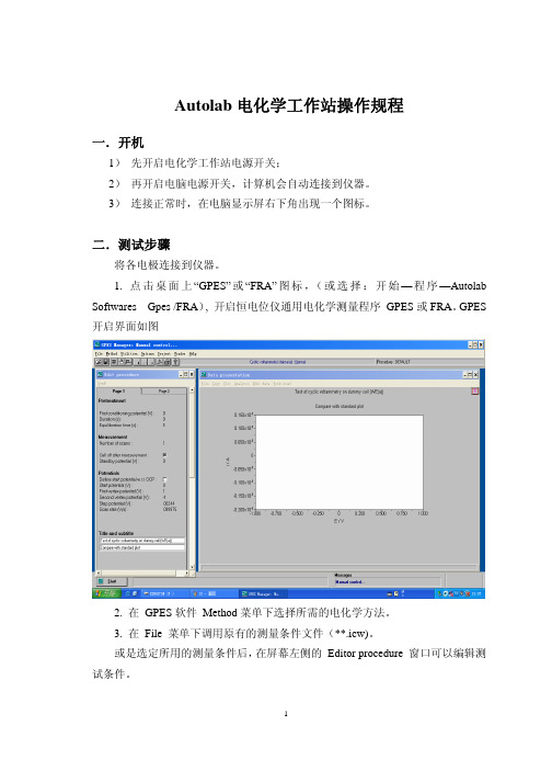
1. 点击桌面上“GPES”或“FRA”图标,(或选择:开始—程序—Autolab Softwares _ Gpes /FRA), 开启恒电位仪通用电化学测量程序 GPES或FRA。
GPES 开启界面如图2. 在 GPES软件 Method菜单下选择所需的电化学方法。
3. 在 File 菜单下调用原有的测量条件文件(**.icw)。
或是选定所用的测量条件后,在屏幕左侧的 Editor procedure 窗口可以编辑测试条件。
First conditioning potential (V)——第一个预处理电位;Duration——在预处理过程中的电位施加时间;Equilibration time——平衡时间。
在预处理后使电极达到平衡的时间;Number of scan ——扫描圈数Standby potential——等候电位。
指在不关闭电极输出时所需要维持的电压;Start potential ——扫描起始电压First vertex potential ——扫描端电压Second vertex potential ——扫描端电压Step potential ——步长Scan rate ——扫速4. 在Editor procedure 窗口的page 2设置文件名,格式为路径+文件名(E:\users\ww\testcv)5. 设定完毕测试条件、再次检查无误后,首先开启仪器上的CELL ENABLE 按钮,再点击屏幕左下角的“Start”按钮,开始测试。
6. 测量结束后,先保存测量结果。
保存方法有三种:a)窗口—File—Save scan as:把测量结果另存为一份文件。
此时,在 CV和 LSV 方法中,每份文件只能保存一个循环的扫描数据(文件后缀为ocw)。
Datacolor AutoLab SPS快速入门手册说明书

Datacolor AutoLab SPS Quick Start ManualPart number: TF-0022-0961Revision 2.01st July 2013Copyright 2007 Datacolor. All Rights Reserved. This material may not be reproduced or copied, in whole or in part, without the written permission of Datacolor.Whilst every effort has been made to ensure the accuracy of this manual, Datacolor can accept no responsibility for any omissions or errors it may contain. Datacolor reserves the right to make improvements and/or changes in the product(s) features and specifications described in this manual at any time.CHAPTER 1: Quick Start (5)CHAPTER 2: Safety (10)Representations and symbols (10)Safety recommendations (11)Document version update log Revision 1New documentRevision 2Change figures of software operationCHAPTER 1: Quick StartLED DisplayMain Power Switch Step 1: Turn on the main power switch, and the “LED Display” will illuminate.HEATER ON ButtonAUTO/MANUAL ButtonStep 2: Check if the “AUTO/MANUAL” button is on, if not, press it to switch it on.Step 3: Make sure target temperature on controller is correct. If not, change it byfollowing steps 4 to 6.Step 4: Press the “SET” button once, the green LED display will flash. Step 5: Press up/down button to set target temperature. Step 6: Press “SET” again to finish temperature setting. Step 7: Check if the hot water tank is full.Step 8:Check if the “HEATER ON” button is on. If not, press it to switch it on. Step 9:Waiting until the actual temperature is same as target temperature shownon controller before stating making solution.Step 10: Start the SPS program to initialize the system.Up/Down ButtonTarget degreesActuality degreesStep 11: Go to link setting to check if SPS link to TF and get data from TF.Step 12: Go to DP Database-> Process for defining a make solution process.Step 13: Go to DP Database-> Solution to set up process, amount to make and fill up use hot water.Step 14: Go SPS Make Solution-> All Bottle List to select the bottle what you want tomake solution. Double click on the bottle for starting to make the selectedsolution.Step 15: Or go to SPS Make Solution-> Make Solution to key in a bottle number tomake a solution.Step 16: Once solution to be made has been selected, placeempty bottle on thescale platform.Step 17: Follow the on-screen messages to complete making the solution.Screen messageCHAPTER 2: SafetyRepresentations and symbolsWarning of a possible danger byheat or steam, which may lead toserious injuryWarning of a possible electric shock,which may lead to serious injuryTips and important rules on thecorrect operation of the system.Datacolor AutoLab SPS Quick-start Manual AutoLab SPS Quick start manual TFSTARTMANSPS / Rev 2.0 / 1st Jul 2013 / Jeffery Fain Page 11 of 11 Safety recommendations•Before turning on the system, make sure that the system operating voltage agrees with the main power voltage. •If the power cable is damaged, the system must be immediately disconnected from the electric supply. •If there is any reason to believe that it is no longer possible to operate the system without danger, the system should be immediately disconnected from the electric supply. •In carrying out maintenance work, it is essentially to heed the maintenance instruction in “Maintenance Guideline”. •If liquid is split into the electric cabinet, connectors or power terminals of the system, the system should be immediately disconnected from main power supply. •Do not put anything inside the main frame of the system that is not intended for use with the system •If any emergency situation should happen, press the “Emergency Button” on the electric cabinet panel to stop the system immediately.。
Autotools使用指南
Autotools使用指南Autotools使用指南一、功能&简介:Linux环境下,我们编译程序啥的都是一般用的GCC&&GDB等等工具,直接使用GCC命令进行编译操作。
这种方式一般是适用于程序文件比较少,组织结构比较简单的情况。
但是,当我们程序文件比较的多的时候,或者是程序文件组织结构比较的复杂(例如在程序文件夹中存在文件夹多层嵌套以及复杂引用等),此时我们如果是直接使用GCC一点一点的编译工作量会非常的大,而且万一程序修改了,还要重新的再工作一遍。
为此,我们有了make工具,依靠Makefile辅助文件,我们可以方便的进行工程的管理,以及编译操作。
当程序很复杂的时候,依靠我们去手工的建立、维护Makefile文件是非常的不现实的,不仅很复杂,而且费时费力,还容易出错。
为此,就有了我们的_Autotools_工具,只要输入工程中的目标文件、依赖文件、文件目录等信息就可以自动生成Makefile。
二、Autotools工具包:Autotools工具包的目标就是去方便的帮助我们得到我们需要的Makefile文件。
___Autotools使用流程:___<1>目录树的最高层运行autoscan,生成configure.scan文件;<2>运行aclocal,生成aclocal.m4文件;<3>运行autoconf,生成configure配置脚本;<4>运行autoheader,生成config.h.in文件;<5>手工编写Makefile.am文件;<6>运行automake,生成Makefile.in;<7>运行配置脚本configure,生成Makefile。
三、c源文件同一目录下Autotools的使用:如果你的源文件都放在同一个目录下面。
可以按照以下步骤来实现同一目录下的Autotools工具的使用:1、编写源代码:2、运行autoscan:第一步:我们需要在我们的<项目目录>下执行autoscan命令。
Autolab电化学工作站仪器的基本操作步骤
Autolab 电化学工作站使用说明1、开机前,检查电化学工作站与电脑的USB接线连接是否正常,保持正确连接。
2、接通电化学工作站主电源,按动电化学工作站前操作面板电源按钮Power键,即打开工作站。
3、启动电脑,并进入Windows操作系统。
4、在启动电脑的同时,电脑会自动检测与电化学工作站的连接情况以及电化学工作站内部设备是否运作正常。
自检完毕后,位于电脑屏幕右下角任务栏处的Autolab之Interface小图标正常显示,可进行下一步操作。
5、进行电化学方法测试前,首先将电化学工作站测量插头(分别是工作电极WE,反馈电极SE,辅助电极CE,参比电极RE)与电解池正确连接,注意电极的正负。
以经典的三电极电解槽为例,其中阴极为测量电极(即工作电解),接线方法为:WE与SE串连接后并与阴极连接,RE与参比电极连接,CE与辅助电极即阳极连接。
6、若进行基本电化学方法测试,点击Autolab之GPES图标,出现该测量界面,进行基本电化学测试,选择相应的Procedure/Method,输入相应的参数,确定参数输入无误后,点击Start按钮,进行测试。
测试完毕后,需要手动保存数据,以免数据丢失,特别需要注意的是保存路径中不能出现中文,否则不能保存数据,也不能打开数据。
7、若进行交流阻抗测试,点击Autolab之FRA图标,出现该测量界面,可行进行交流阻抗测试,选择相应的Procedure/Method,输入相应的参数,确定参数输入无误后,点击Start按钮,进行测试。
测试完毕后,需要手动保存数据,操作同一。
8、在测试间隙待机状态下,四根电极接线不宜空置,需要与实际体系连接,或插回Dummy Cell中,防止短路。
9、测试结束后,关闭电化学工作站的基本操作为:首先关闭软件操作界面,退出软件后,关闭电化学工作站前操作面板的电源按钮Power键,即关闭电化学工作站,最后切断电源。
- 1、下载文档前请自行甄别文档内容的完整性,平台不提供额外的编辑、内容补充、找答案等附加服务。
- 2、"仅部分预览"的文档,不可在线预览部分如存在完整性等问题,可反馈申请退款(可完整预览的文档不适用该条件!)。
- 3、如文档侵犯您的权益,请联系客服反馈,我们会尽快为您处理(人工客服工作时间:9:00-18:30)。
电化学工作站软件简要操作手册(版本:4.9.005)目录一软件的安装 (6)二简要操作说明 (11)1.开机步骤 (11)2.GPES操作步骤 (11)3.FRA操作步骤 (14)三GPES软件 (15)1.窗口 (15)2.手动控制窗口 (24)3.测量条件窗口 (25)4.数据分析窗口 (26)四FRA软件 (38)1.主窗口 (38)2.手动控制窗口 (43)3.FRA设置窗口 (44)4.FRA手动控制窗口 (44)5.测量条件窗口 (45)6.数据分析窗口 (47)五电化学技术手册 (55)1. Autolab电化学试验 (55)2. 伏安分析 (57)3. 循环和线性扫描伏安 (62)4. 记时方法 (65)5. 多模式电化学检测 (67)6. 电位溶出分析 (68)7. 阶跃与扫描 (69)8. 电化学噪声 (70)9. 使用FRA模块的频率响应分析 (71)10. 高级技术 (74)附录一: GPES软件参数说明 (78)附录二: FRA软件参数说明 (93)附录三:FRA中的模拟与拟合 (96)注意事项1. 四根电极接线不能空置!只能与实际体系连接,或插回Dummy Cell中。
2. 在采用两电极体系时,WE与S相连接,RE与CE相连接;采用三电极体系时,WE与S仍然相连接;仅在四电极体系时才分开。
3. 保存文件时,由路径至文件名称都不能有中文字符!否则不能打开文件。
4. 在保存文件功能上,对于循环伏安或线性扫描方法,提供下述三种保存方式,其余的仅有(1)和(3)两种方式:(1) “主窗口——Files菜单——Save scan as”,把每一圈的数据保存为一份文件,以方便对曲线进行分析;(2) “主窗口——Files菜单——Save data as——Save data buffer as”,可把多圈扫描结果保存在同一份文件之中,以方便对不同扫描圈的数据进行对比。
这种文件打开时需要用“主窗口——Files菜单——Loaddata buffer”命令。
(3) “Data Presetation窗口——File菜单——Save work data保存工作数据”,此时保存的是经修饰后的数据结果。
5. 在GPES软件中,保存文件时,会自动保存三份文件:*.i?i、*.i?w、*.o?w;在FRA软件中,保存文件时会自动保存两份文件:*.dfr、*.pfr。
在复制文件是必须三份文件(或两份)全部复制!否则无法打开文件。
第一章软件的安装1. 首先,不要把仪器与电脑相连接,等安装程序完成并重启电脑后才插入USB连线。
2. 把原版的AUTOLAB软件光盘放入电脑光驱之中,可自动运行。
3. 选择“首次安装软件”;4. 显示如下,按“NEXT”5. 显示“软件产品声明”,按“Yes”:6. 显示“自述文件”,按“NEXT”:7. 选择“程序的安装路径”,通常默认C盘根目录下;8. 选择相应的软件功能。
其中,Gpes 和Diagnostics是必需的程序。
Fra则要求带有FRA模块的仪器才需要安装。
Mutlichannel只应用于多通道型仪器上。
9. 选择“仪器接口形式”,在2003年后的产品,基本上采用USB接口,因此,选择默认的选项“Autolab-USB(Internal)or Autolab-USB Interfacebox”。
按“NEXT”进入下一步。
10. 选择在Windows系统开始菜单中的快捷模式,然后按“NEXT”进入下一步安装过程。
11. 如果以前已安装过AUTOLAB软件,则会出现以下界面,允许用户选择是否把原有的目录备份。
12. 然后,出现界面,请再确认本仪器的配置。
13. 显示配置面板,根据仪器的实际配置选择相应的项目。
通常情况下可以选择默认方式。
(因基本上会把相应客户的配置文件已复制于本光盘内)14. 安装完成后,按Finish:15. 如果在第一步中软件还有升级版本,则选择“No,Iwill restart my computerlater”,按“Finish”进入第15步。
否则,选择“Yes,I want to restart mycomputer now”,按“Finish”。
进入下一步。
16. 选择“升级软件”,按照提示进行相应的操作。
最后,回到第13步。
17. 电脑重启后,电脑会显示连接错误。
此时,再打开仪器电源,并把USB线插入电脑USB接口中。
18. 在Windows ME/2000/XP系统下,电脑会显示“发现新硬件”。
选择“指定路径和目录”,按“下一步”。
选择目录“C:/AUTOLAB/USB”,安装在该目录下的驱动程序。
此步骤需重复执行两次。
19. 按鼠标右键点击桌面右下角的界面图标,选择“Restore——Refresh”重新连接。
正常状态下应该可以连接正常。
把该窗口最小化。
20. 如果是新版的软件,软件还会自动对仪器的接口模块进行检测是否需要升级,如需要升级,请具体根据图示进行。
注:在升级过程中必须保证电脑及仪器的电源正常!否则会损坏仪器的接口模块!第二章简要操作说明一开机1)先开启电化学工作站电源开关;2)再开启电脑电源开关,出现如下图显示框,计算机会自动连接到仪器。
3)连接正常时,在电脑显示屏右下角出现图标。
二测试步骤1 General Purpose Electrochemical Software (GPES通用电化学软件)1.1 点击桌面上图标,(或:开始——程序——Autolab Softwares——Gpes),开启恒电位仪通用电化学测量程序GPES。
1.2 在GPES软件Method菜单下选择所需的电化学方法。
1.3 在File菜单下调用原有的测量条件文件。
1.4 选定所用的测量条件文件后,在屏幕左侧的Edit procedure窗口可以编辑测试条件。
(具体的测量条件含义详见附件)。
1.5 在Manual control(手工控制)对话框中,选择合适的项目。
1.6 设定完毕测试条件,再次检查无误后,点击屏幕左下角的按钮,开始测试。
1.7 测量结束后,先保存测量结果。
对于CV和LSV方法,保存方式有三种,其余的只有1、3两种:a) 窗口——File——Save scan as:把测量结果另存为一份文件。
此时,在CV和LSV方法中,每份文件只能保存一个循环的扫描数据。
并且,此种方式仅能保存原始数据。
b) 主窗口——File——Save data——Save data buffer as:把缓存器中的数据保存为一份缓存文件。
此时,在CV和LSV测试中,一份文件可以有多个循环的扫描结果。
c) Data presetation窗口——File——Save work data:此时可保存经修饰后的数据,包括曲线平滑、删除某些误点等。
1.8 各种曲线的分析。
2 Frequency Response Analyser Software(FRA电化学阻抗软件)2.1 点击“开始——程序——Autolab Softwares——Fra”,开启FRA分析软件。
2.2 在Method菜单下选择所需的分析方法2.3 在File菜单下调用原有的测量条件文件。
2.4 在Edit frequencies对话框内,设置相应的测试参数:说明:此对话框内,可以设定开始扫描频率(begin fre)和终止频率(end fre),并根据两者的差值来确定测量的频率点数,(推荐选择每一个数量级取10个频率,总频数=数量级数X10+1),点击计算(Calculate),如果需要也可以重新设置所需的具体频率值。
设定完毕后点击OK即可(推荐:begin fre为高频,而end fre为低频)。
2.5 在Edit precedure对话框内,设置处理及测试条件。
2.6 设定完毕后,点击按钮开始测量。
2.7 软件会出现默认的Z’ ~ -Z”图,可以选择菜单“Data Presentation——View”中,打开其他所需的曲线图,常用Bode图。
2.8 测量完成后,先保存数据,以免软件出错而造成数据丢失。
2.9 对曲线进行各种分析。
第三章GPES 软件1 主窗口:1.1 文件菜单File1.1.1 Open procedure打开测量条件测量条件是作为一份独立的文件保存,该文件包含了所有的测量参数,1.1.2 Save procedure保存测量条件允许用户把修改的测量条件保存在当前目录下。
1.1.3 Save procedure as另存测量条件允许用户把修改的测量条件另存在自选的目录下。
1.1.4 Print打印直接在所连接的打印机打印所选择的内容。
打印格式默认为GPES标准模版,如右图所示。
1.1.5 Print setup打印设置设置打印的模式。
1.1.6 Load data (或Load scan)调用测量数据结果允许调用所保存的测量数据。
也可以按<Shift>或<Control>键,多选文件,以便直接进行叠加显示。
(最多10份文件)1.1.7 Load data buffer调用数据缓存文件允许调用所保存的数据缓存文件。
在CV和LSV测量时,这种文件可同时保存多个扫描的数1.1.8 Save data (或Save scan as)保存测量结果通常状态下,允许保存测量结果。
在CV或LSV状态时,用户可选择保存多个扫描中的某一扫描。
1.1.9 Save data as另存数据1.1.9.1 Save data buffer as保存缓存文件在CV或LSV下,把多圈扫描保存在同一份数据缓存文件之中。
1.1.9.2 Export to scanno. Vs Q+,Q- file输出为扫描次数~ 阴阳极交换电量的文件允许用户把测量数据以“扫描次数~阴阳极交换电量”的格式保存,方便对不同扫描的交换电量进行分析。
1.1.9.3 Export Chrono data输出为记时文件此选项仅在CV时。
在CV测量时,允许用户设定在边界电位下进行记时测量。
因此,本选项供用户把此时的记时测量结果单独保存。
1.1.9.4 Export to BAS-DigiSim data输出为BAS-DigiSim格式文件仅在CV时。
允许用户把数据保存为DigiSim软件能读取的格式。
这是一种带有默认扩展名(.TXT)的ASCII文件。
1.1.9.5 Export data buffer to text file把数据缓存文件输出为文本文档仅用于CV或LSV下。
可把数据缓存文件输出为普通的文本文档格式。
1.1.10 Delete Files删除文件允许用户删除测量条件及测量数据文件。
删除时,仅显示条件文件,但可同时把对应的数据文件也删除。