1 Stock Return Regressions Rt+1rt = a+b1x1t+b2x2t+...+bkxkt+εt+1, (1)
计量经济学第三版课后习题答案第二章 经典单方程计量经济学模型:一元线性回归模型

第二章经典单方程计量经济学模型:一元线性回归模型一、内容提要本章介绍了回归分析的基本思想与基本方法。
首先,本章从总体回归模型与总体回归样本回归模型与样本回归函数这两组概念开始,在现实中只能先从总体中抽取一个样本,本章的一个重点是如何获取线性的样本回归函数,主要涉及到普通最小二乘法(本章的另一个重点是对样本回归函数能否代表总体回归函数进行统计推断,即进行所统计检验包括两个方面,本章还有三方面的内容不容忽视。
其一,若干基本假设。
样本回归函数参数的估计以参数估计量统计性质的分析,例1、令kids运用样本回归函数进行预测,建立了回归分析的基本思想。
由总体回归模型在若干基本假设下得到,获得样本回归函数,ML)以及矩估计法(一是先检验样本回归函数与样本点的Goss-markov包括被解释变量条件均值与个educ表示该妇女接受过教育的年数。
生总体回但它只是并用它对总OLS)MM)。
“拟合优度”,t检验完成;第二,OLS估计量1函数、归函数是对总体变量间关系的定量表述,建立在理论之上,体回归函数做出统计推断。
的学习与掌握。
同时,也介绍了极大似然估计法(谓的统计检验。
第二是检验样本回归函数与总体回归函数的“接近”程度。
后者又包括两个层次:第一,检验解释变量对被解释变量是否存在着显著的线性影响关系,通过变量的检验回归函数与总体回归函数的“接近”程度,通过参数估计值的“区间检验”完成。
及对参数估计量的统计性质的分析以及所进行的统计推断都是建立在这些基本假设之上的。
其二,包括小样本性质与大样本性质,尤其是无偏性、有效性与一致性构成了对样本估计量优劣的最主要的衡量准则。
定理表明是最佳线性无偏估计量。
其三,值的预测,以及预测置信区间的计算及其变化特征。
二、典型例题分析表示一名妇女生育孩子的数目,育率对教育年数的简单回归模型为(1)随机扰动项包含什么样的因素?它们可能与教育水平相关吗?(2)上述简单回归分析能够揭示教育对生育率在其他条件不变下的影响吗?请解释。
计量经济学考试题
(3)对数—线性模型:
对数—线性模型又称增长模型,X变化一个单位,Y变化B2个百分点; (4分)
(4)线性—对数模型:
X变化一个百分点,Y变化0.01×B2个单位。 (4分)
2.(12分)答:(1)不是。因为农村居民储蓄增加额应与农村居民可支配收入总额有关,而与城镇居民可支配收入总额之间没有因果关系。
(3)
令:资本的产出弹性记为B。
H0:B=0.5,H1:B 0.5
查表得:
而5.2>1.96, (5分)
所以拒绝H0:B=0.5,接受H1:B 0.5。 (2分)
(4)由上表结果,可知F统计量的值为1628,相应的尾概率为0.0000<0.05,故模型是总体显著的。 (4分)
(5)根据模型结果可知:某国在1980—2001年间,资本的产出弹性约为0.76,即在其他情况不变的条件下,资本投入每增加一个百分点,产出平均提高0.76个百分点。 (3分)劳动投入的产出弹性为0.64,即在其他条件不变的条件下,劳动投入每增加一个百分点,产出平均提高0.64个百分点。 (3分)
4.答:(1)间接二乘法适用于恰好识别方程,而两阶段最小二乘法不仅适用于恰好识别方程,也适用于过度识别方程;(2)间接最小二乘法得到无偏估计,而两阶段最小二乘法得到有偏的一致估计;都是有限信息估计法。
5.答:对模型参数施加约束条件后,就限制了参数的取值范围,寻找到的参数估计值也是在此条件下使残差平方和达到最小,它不可能比未施加约束条件时找到的参数估计值使得残差平方达到的最小值还要小。但当约束条件为真时,受约束回归与无约束回归的结果就相同了。
2.答:显著性检验分模型的拟合优度检验和变量的显著性检验。前者主要指标为可决系数以及修正可决系数,后者主要通过计算变量斜率系数的t统计量进行检验……
计量经济学试题(库)(超完整版)与答案解析

四、简答题(每小题5分)1.简述计量经济学与经济学、统计学、数理统计学学科间的关系。
2.计量经济模型有哪些应用? 3.简述建立与应用计量经济模型的主要步骤。
4.对计量经济模型的检验应从几个方面入手?5.计量经济学应用的数据是怎样进行分类的? 6.在计量经济模型中,为什么会存在随机误差项?7.古典线性回归模型的基本假定是什么? 8.总体回归模型与样本回归模型的区别与联系。
9.试述回归分析与相关分析的联系和区别。
10.在满足古典假定条件下,一元线性回归模型的普通最小二乘估计量有哪些统计性质? 11.简述BLUE 的含义。
12.对于多元线性回归模型,为什么在进行了总体显著性F 检验之后,还要对每个回归系数进行是否为0的t 检验?13.给定二元回归模型:01122t t t ty b b x b x u =+++,请叙述模型的古典假定。
14.在多元线性回归分析中,为什么用修正的决定系数衡量估计模型对样本观测值的拟合优度? 15.修正的决定系数2R 及其作用。
16.常见的非线性回归模型有几种情况? 17.观察下列方程并判断其变量是否呈线性,系数是否呈线性,或都是或都不是。
①t t t u x b b y ++=310 ②t t t u x b b y ++=log 10 ③ t t t u x b b y ++=log log 10 ④t t t u x b b y +=)/(1018. 观察下列方程并判断其变量是否呈线性,系数是否呈线性,或都是或都不是。
①t t t u x b b y ++=log 10 ②t t t u x b b b y ++=)(210 ③ t t t u x b b y +=)/(10 ④t b t t u x b y +-+=)1(110 19.什么是异方差性?试举例说明经济现象中的异方差性。
20.产生异方差性的原因及异方差性对模型的OLS估计有何影响。
21.检验异方差性的方法有哪些?22.异方差性的解决方法有哪些?23.什么是加权最小二乘法?它的基本思想是什么?24.样本分段法(即戈德菲尔特——匡特检验)检验异方差性的基本原理及其使用条件。
计量经济学题库(超完整版)及答案

A.异方差问题B.序列相关问题C.多重共线性问题D.设定误差问题
70.设回归模型为 ,其中 ,则 的最有效估计量为()
A. B. C. D.
71.如果模型yt=b0+b1xt+ut存在序列相关,则()。
A. cov(xt, ut)=0 B. cov(ut, us)=0(t≠s) C. cov(xt, ut)≠0 D. cov(ut, us)≠0(t≠s)
A.重视大误差的作用,轻视小误差的作用B.重视小误差的作用,轻视大误差的作用
C.重视小误差和大误差的作用D.轻视小误差和大误差的作用
68.如果戈里瑟检验表明,普通最小二乘估计结果的残差 与 有显著的形式 的相关关系( 满足线性模型的全部经典假设),则用加权最小二乘法估计模型参数时,权数应为()
A. B. C. D.
53.线性回归模型 中,检验 时,所用的统计量 服从( )
A.t(n-k+1) B.t(n-k-2)C.t(n-k-1) D.t(n-k+2)
54. 调整的判定系数 与多重判定系数 之间有如下关系()
A. B.
C. D.
55.关于经济计量模型进行预测出现误差的原因,正确的说法是( )。
A.只有随机因素 B.只有系统因素 C.既有随机因素,又有系统因素 D.A、B、C 都不对
23.产量(X,台)与单位产品成本(Y,元/台)之间的回归方程为 ,这说明()。
A.产量每增加一台,单位产品成本增加356元B.产量每增加一台,单位产品成本减少1.5元
C.产量每增加一台,单位产品成本平均增加356元D.产量每增加一台,单位产品成本平均减少1.5元
24.在总体回归直线 中, 表示()。
计量经济学:一元线性回归模型和多元线性回顾模型习题以及解析

第二章经典单方程计量经济学模型:一元线性回归模型一、内容提要本章介绍了回归分析的基本思想与基本方法。
首先,本章从总体回归模型与总体回归函数、样本回归模型与样本回归函数这两组概念开始,建立了回归分析的基本思想。
总体回归函数是对总体变量间关系的定量表述,由总体回归模型在若干基本假设下得到,但它只是建立在理论之上,在现实中只能先从总体中抽取一个样本,获得样本回归函数,并用它对总体回归函数做出统计推断。
本章的一个重点是如何获取线性的样本回归函数,主要涉及到普通最小二乘法(OLS)的学习与掌握。
同时,也介绍了极大似然估计法(ML)以及矩估计法(MM)。
本章的另一个重点是对样本回归函数能否代表总体回归函数进行统计推断,即进行所谓的统计检验。
统计检验包括两个方面,一是先检验样本回归函数与样本点的“拟合优度”,第二是检验样本回归函数与总体回归函数的“接近”程度。
后者又包括两个层次:第一,检验解释变量对被解释变量是否存在着显著的线性影响关系,通过变量的t检验完成;第二,检验回归函数与总体回归函数的“接近”程度,通过参数估计值的“区间检验”完成。
本章还有三方面的内容不容忽视。
其一,若干基本假设。
样本回归函数参数的估计以及对参数估计量的统计性质的分析以及所进行的统计推断都是建立在这些基本假设之上的。
其二,参数估计量统计性质的分析,包括小样本性质与大样本性质,尤其是无偏性、有效性与一致性构成了对样本估计量优劣的最主要的衡量准则。
Goss-markov定理表明OLS估计量是最佳线性无偏估计量。
其三,运用样本回归函数进行预测,包括被解释变量条件均值与个值的预测,以及预测置信区间的计算及其变化特征。
二、典型例题分析例1、令kids表示一名妇女生育孩子的数目,educ表示该妇女接受过教育的年数。
生育率对教育年数的简单回归模型为β+μβkids=educ+1(1)随机扰动项μ包含什么样的因素?它们可能与教育水平相关吗?(2)上述简单回归分析能够揭示教育对生育率在其他条件不变下的影响吗?请解释。
李子奈计量经济学课后答案

i
GDPi
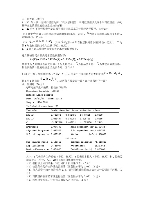
其中, GDPi (i 1,2,3) 是第 i 产业的国内生产总值。 (2) S1 S 2 其中, S1 、 S 2 分别为农村居民和城镇居民年末储蓄存款余额。 (3) Yt 1 I t 2 Lt 其中, Y 、 I 、 L 分别为建筑业产值、建筑业固定资产投资和职工人数。 (4) Yt Pt 其中, Y 、 P 分别为居民耐用消费品支出和耐用消费品物价指数。 (5) 财政收入 f (财政支出) (6) 煤炭产量 f ( L, K , X 1 , X 2 ) 其中, L 、 K 分别为煤炭工业职工人数和固定资产原值, X 1 、 X 2 分别为发电量和钢铁产 量。 1-20.模型参数对模型有什么意义?
5
第二章
经典单方程计量经济学模型:一元线性回归模型
Байду номын сангаас
一、内容提要
本章介绍了回归分析的基本思想与基本方法。首先,本章从总体回归模型与总体回归 函数、样本回归模型与样本回归函数这两组概念开始,建立了回归分析的基本思想。总体回 归函数是对总体变量间关系的定量表述, 由总体回归模型在若干基本假设下得到, 但它只是 建立在理论之上,在现实中只能先从总体中抽取一个样本,获得样本回归函数,并用它对总 体回归函数做出统计推断。 本章的一个重点是如何获取线性的样本回归函数,主要涉及到普通最小二乘法(OLS) 的学习与掌握。同时,也介绍了极大似然估计法(ML)以及矩估计法(MM) 。 本章的另一个重点是对样本回归函数能否代表总体回归函数进行统计推断,即进行所 谓的统计检验。统计检验包括两个方面,一是先检验样本回归函数与样本点的“拟合优度” , 第二是检验样本回归函数与总体回归函数的“接近”程度。后者又包括两个层次:第一,检 验解释变量对被解释变量是否存在着显著的线性影响关系,通过变量的 t 检验完成;第二, 检验回归函数与总体回归函数的“接近”程度,通过参数估计值的“区间检验”完成。 本章还有三方面的内容不容忽视。其一,若干基本假设。样本回归函数参数的估计以 及对参数估计量的统计性质的分析以及所进行的统计推断都是建立在这些基本假设之上的。 其二,参数估计量统计性质的分析,包括小样本性质与大样本性质,尤其是无偏性、有效性 与一致性构成了对样本估计量优劣的最主要的衡量准则。 Goss-markov 定理表明 OLS 估计量 是最佳线性无偏估计量。其三,运用样本回归函数进行预测,包括被解释变量条件均值与个 值的预测,以及预测置信区间的计算及其变化特征。
3.计量经济学第三讲-双变量线性回归模型

第一节、双变量线性回归模型的估计 二.普通最小二乘法(OLS法)
1. 双变量线性回归模型的统计假设
设双变量线性回归模型 (the two variable linear regression model)
Yt = + Xt + ut,t = 1, 2, …, n
第一节、双变量线性回归模型的估计
二.普通最小二乘法(OLS法) 1. 双变量线性回归模型的统计假设
假设5:各期扰动项ut的方差相等。即
Var(ut) = E{[ut-E(ut)]2} = E(ut2) = σ2 — 假设3 t = 1, 2, …, n
Tuesday, 7 Oct. 2008 CUFE
3、模型的确定部分和随机部分
在计量经济学中,我们专门研究变量间的随 机性关系,如: Yt = + Xt + ut,t = 1, 2, …, n 这些随机性关系往往可以分成两个部分:一 部分是非随机部分,如式中的 + Xt就是Yt的 是非随机部分,称为模型的确定部分或系统部分, 而另一部分是均值为零的随机部分即随机扰动项 ut。 我们通常假定X为非随机变量,而Y,因其 包含随机扰动项ut,则为随机变量。在非随机变 量X一定的条件下,随机变量Y的系统部分为X 的线性函数。实际上,随机变量Y的系统部分就 是Y在非随机变量X一定的条件下的数学期望。
Tuesday, 7 Oct. 2008 CUFE
Demand function
“A relationship which shows mathematically how the quantity demanded of a good or service responds to changes in a number of economic factors such as its own price, the prices of substitutes and complementary goods, income, credit terms, etc. The quantity demanded is the dependent variable and the other factors are independent variables. The effect of each independent variable on the dependent variable may be estimated statistically by time-series analysis or cross-section analysis of household expenditure data.”
计量经济学期末复习资料
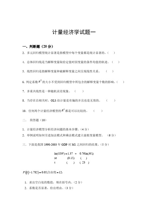
计量经济学试题一一、判断题(20分)2.多元回归模型统计显著是指模型中每个变量都是统计显著的。
( ) 4.总体回归线是当解释变量取给定值时因变量的条件均值的轨迹。
( ) 5.线性回归是指解释变量和被解释变量之间呈现线性关系。
( ) 6.判定系数的大小不受到回归模型中所包含的解释变量个数的影响。
( ) 7.多重共线性是一种随机误差现象。
( )8.当存在自相关时,OLS 估计量是有偏的并且也是无效的。
( ) 10.任何两个计量经济模型的都是可以比较的。
( ) 二. 简答题(10)1.计量经济模型分析经济问题的基本步骤。
(4分)2.举例说明如何引进加法模式和乘法模式建立虚拟变量模型。
(6分) 三.下面是我国1990-2003年GDP 对M1之间回归的结果。
(5分)1.求出空白处的数值,填在括号内。
(2分) 2.系数是否显著,给出理由。
(3分)2R 2R ln() 1.37 0.76ln(1)se (0.15) ( )t ( ) ( 23 )GDP M =+()1.7820.05,12P t >==自由度;四.试述异方差的后果及其补救措施。
(10分)五.多重共线性的后果及修正措施。
(10分)六.试述D-W检验的适用条件及其检验步骤?(10分)八、(20分)应用题为了研究我国经济增长和国债之间的关系,建立回归模型。
得到的结果如下:Dependent Variable: LOG(GDP)Method: Least SquaresDate: 06/04/05 Time: 18:58Sample: 1985 2003Included observations: 19Variable Coefficient Std. Error t-Statistic Prob.LOG(DEBT) 0.65 0.02 32.8 0Adjusted R-squared 0.983 S.D. dependent var 0.86 S.E. of regression 0.11 Akaike info criterion -1.46 Sum squared resid 0.21 Schwarz criterion -1.36 Log likelihood 15.8 F-statistic 1075.5 Durbin-Watson stat 0.81 Prob(F-statistic) 0L U其中,GDP表示国内生产总值,DEBT表示国债发行量。
- 1、下载文档前请自行甄别文档内容的完整性,平台不提供额外的编辑、内容补充、找答案等附加服务。
- 2、"仅部分预览"的文档,不可在线预览部分如存在完整性等问题,可反馈申请退款(可完整预览的文档不适用该条件!)。
- 3、如文档侵犯您的权益,请联系客服反馈,我们会尽快为您处理(人工客服工作时间:9:00-18:30)。
Mphil Subject301 Market Efficiency and Stock MarketPredictabilityM.Hashem PesaranMarch200311Stock Return Regressions R t+1−r t=a+b1x1t+b2x2t+...+b k x kt+εt+1,(1) R t+1is the one-period(day,week,month,..) holding return on an stock index,such as FTSE,Dow Jones or Standard and Poor500, defined byR t+1=(P t+1+D t+1−P t)/P t,(2) P t is the stock price at the end of the period and D t+1is the dividend paid out over the period t to t+1,and x it,i=1,2,...,k are the factors/variables thought to be important in predicting stock returns.Finally,r t is the return on the government bond with one-period to maturity(the period to maturity of the bond should exactly be the same as the holding period of the stock).R t+1−r t is known as the excess return(return on stocks in excess of the return on the safe asset). Note also that r t would be known to the2investor/trader at the end of period t,beforethe price of stocks,P t+1,is revealed at the endof period t+1.Examples of possible stock marketpredictors are past changes in macroeconomic variables such as interest rates,inflation,dividend yield(D t/P t−1),price earningsratio,output growth,and term premium(the difference in yield of a high grade and a lowgrade bond such as AAA rated minus BAArated bonds).For individual stocks the relevant stockmarket regression is the capital asset pricingmodel(CAPM),augmented with potential predictors:R i,t+1=a i+b1i x1t+b2i x2t+...+b ki x kt+βi R t+1+εi,t+1,(3) where R i,t+1is the holding period return onasset i(shares offirm i),defined similarlyas R t+1.The asset-specific regressions(3)could also includefirm specific predictors,such as R it or its higher order lags,book-to-3market value or size offirm i.Under market efficiency,as characterized by CAPM,a i=0,b1i=b2i=....=b ki=0. Only the“betas”,βi,will be significantly different from zero.Under CAPM,the value ofβi captures the risk of holding the share i with respect to the market.2Market Efficiency and Stock Market Predictability It is often argued that if stock markets areefficient then it should not be possible to predict stock returns,namely that none of the variables in the stock market regression (1)should be statistically significant.Some writers have even gone so far as to equate stock market efficiency with the non-predictability property.But this line of argument is not satisfactory and does not help in furthering our understanding of how markets operate. The concept of market efficiency needs to be4defined separately from predictability.In fact, it is easily seen that stock market returns will be non-predictable only if market efficiency is combined with risk neutrality.2.1Risk Neutral Investors Suppose there exists a risk free asset such as a government bond with a known payout.In such a case an investor with an initial capital of£A t,is faced with two options:•Option1:holding the risk-free asset andreceiving$(1+r t)A t,at the end of the next period,•Option2:switching to stocks by purchasingA t/P t shares and holding them for oneperiod and expecting to receive$(A t/P t)(P t+1+D t+1),at the end of period t+1.A risk-neutral investor will be indifferent between the certainty of$(1+r t)A t,and the5his/her expectations of the uncertain payout of ly,for such a risk neutral investor(1+r t)A t=E[(A t/P t)(P t+1+D t+1)|I t],(4) where I t is the investor’s information at the end of period t.This relationship is called the “Arbitrage Condition”.Using(2)we now haveP t+1+D t+1=P t(1+R t+1),and the above arbitrage condition can be simplifies toE[(1+R t+1)|I t]=(1+r t),orE(R t+1−r t|I t)=0.(5) This result establishes that if the investor forms his/her expectations of future stock (index)returns taking account of all market information efficiently,then the excess return, R t+1−r t,should not be predictable using any of the market information that are available at the end of period t.Notice that r t is known6at time t and is therefore included in I t .Hence,under the joint hypothesis of market ef ficiency and risk neutrality we must also have E (R t +1|I t )=r t .The above set up can also be used to derive conditions under which asset prices can be characterised as a random walk model.Suppose,the risk free rate,r t ,in addition to being known at time t ,is also constant over time.Then using(4)we can also write P t =µ11+r ¶(E [(P t +1+D t +1)|I t ]),or P t =µ11+r ¶[E (P t +1|I t )+E (D t +1|I t )].Under the rational expectations hypothesis andassuming that the “transversality condition”lim j →∞µ11+r ¶j E (P t +j |I t )=0holds we have the familiar result P t =∞X j =1µ11+r ¶j E (D t +j |I t ),7that equates the level of stock price to the present discounted stream of the dividends expected to occur to the asset over the infinite future.The transversality condition rules out rational speculative bubbles and is satisfied if the asset prices are not expected to rise faster than the exponential decay rate determined by the discount factor,0<1/(1+r)<1.It is now easily seen that if D t follows a random walk so will P t.For example,supposeD t=D t−1+εt,whereεt+1is a white noise process.ThenE(D t+j|I t)=D t,andP t=D t r.Therefore,we also haveP t=P t−1+u t,where u t=εt/r.The random walk property holds even if r=0,since in such a case it would be reasonable to expect no dividends are also8paid out,namely D t=0.In this case the arbitrage condition becomesE(P t+1|I t)=P t,(6) which is satisfied by the random walk modelbut is in fact more general than the randomwalk model.An asset price that satisfies(6)is said to be a martingale process.Randomwalk processes with zero drift are martingale processes but not all martingale processes are random walks.For example,the price process P t+1=P t+λn(∆P t+1)2−E h(∆P t+1)2|I t io+εt, whereεt is a white noise process is a martin-gale process with respect to the informationset I t,but it is clearly not a random walk process,unlessλ=0.2.2Risk Averse InvestorsRisk neutrality is a behavioral assumption and need not hold even if all market informationis processed efficiently by all the market participants.A more reasonable way to proceed is to allow some or all the investors9to be risk averse.In this more generalcase the certain pay out,(1+r t)A t,andthe expectations of the uncertain pay out,E[(A t/P t)(P t+1+D t+1)|I t],will not be the same and differ by a(possibly)time-varyingrisk premium which could also vary withthe level of the initial capital,A t.Morespecifically,we haveE[(A t/P t)(P t+1+D t+1)|I t]=(1+r t)A t+λt A t, whereλt is the premium per$of invested capital required(expected)by the investor.Itis now easily seen thatE(R t+1−r t|I t)=λt,and it is no longer necessary true that under market efficiency excess returns are non-predictable.The extent to which excess returns can be predicted will depend on the existence of a historically stable relationship between the risk premium,λt,and the macro and business cycle indicators such as changesin interest rates,dividends and various business cycle indicators.10Market inefficiencies provide furthersources of stock market predictability byintroducing a wedge between a“correct”exante measure of E(R t+1−r t|I t),and its estimate by market participants.Denoting thelatter byˆE(R t+1−r t|I t)we haveE(R t+1−r t|I t)=λt+ξt, whereξt=E(R t+1|I t)−ˆE(R t+1|I t), andξt measures the extent to which errors are made by market participants in predicting stock returns.In practice,ˆE(R t+1|I t)is likely to be a weighted“average”ofmarket participants’returns expectations(formed possibly with respect to differentinformations,all being the sub-set of I t).The weights will be determined by the investor’s market share(positive if they are long and negative if they are short).Similarly,λt,is the weighted average of the risk premium(per£invested)of the different market participants.113Evidence of Stock Market PredictabilityEconomists have long been fascinated by the sources of variations in the stock market.By the early1970’s a consensus had emerged amongfinancial economists suggesting that stock prices could be well approximated by a random walk model and that changes in stock returns were basically unpredictable. Fama(1970)provides an early,definitive statement of this position.Historically,the ‘random walk’theory of stock prices was preceded by theories relating movementsin thefinancial markets to the business cycle.A prominent example is the interest shown by Keynes in the variation in stock returns over the business cycle.According to Skidelsky(1992)“Keynes initiated what was called an‘Active Investment Policy’,which combined investing in real assets-at that time considered revolutionary-with constant12switching between short-dated and long-dated securities,based on predictions of changes in the interest rate”(Skidelsky(1992,p.26)).Recently,a large number of studies in the finance literature have confirmed that stock returns can be predicted to some degree by means of interest rates,dividend yields and a variety of macroeconomic variables exhibiting clear business cycle variations.While the vast majority of these studies have looked at the US stock market,an emerging literature has also considered the UK stock market.US Studies include Balvers,Cosimano and MacDonald(1990),Breen,Glosten and Jagannathan(1990),Campbell(1987), Fama and French(1989),Ferson and Harvey (1993),and Pesaran and Timmermann(1994, 1995).See Granger(1992)for a survey of the methods and results in the literatureUK Studies include Clare,Thomas and Wickens(1994),Clare,Psaradakis and Thomas(1995),Black and Fraser(1995),and13Pesaran and Timmermann(2000).4ExerciseThefile UKUS.fit contains monthly observa-tions on UK and US ing the available data,investigate the extent to which stock markets in UK and US could have been predicted during1990’s.5Pitfalls and Problems •Data mining/Data snooping•Structural change and model instability •Transaction costs and market predictability •Market volatility and learning14REFERENCESBalvers,R.J.,Cosimano,T.F.and MacDonald,B.(1990)“Predicting Stock Returns in an Efficient Market”.Journal of Finance,45,1109-28.Black,A.and Fraser,P.(1995)”UK Stock Returns:Predictability and Business Conditions”. The Manchester School Supplement,85-102.Breen,W.,L.R.Glosten,and R.Jagannathan(1990)“Predictable Variations in Stock Index Returns”.Journal of Finance,44,1177-1189.Brennan,M.J.,Schwartz,E.S.,and Lagnado,R.(1997)”Strategic Asset Allocation”.Journal of Economic Dynamics and Control,21,1377-1403.Buckle,M.G.,Clare,A.D.,and Thomas,S.H.(1994)”Predicting the Returns from Stock Index Futures”.Discussion Paper94-04,Brunel.Bulkley,G.and Harris,R.D.F.(1997)”Irrational Analysts’Expectations as a Cause of Excess V olatility in Stock Prices”.Forthcoming in Economic Journal.Bulkley,G.and Tonks,I.(1989)“Are UK Stock Prices Excessively V olatile?Trading Rules and Variance Bounds Tests”.The Economic Journal,vol.99,1083-98.Campbell,J.Y.(1987)“Stock Returns and the Term Structure”.Journal of Financial Economics,373-99.Clare,A.D.,Thomas,S.H.,and Wickens,M.R.(1994)“Is the Gilt-Equity Yield Ratio Useful for Predicting UK Stock Return?”.Economic Journal,104,303-15.Clare,A.D.,Psaradakis,Z.,and Thomas,S.H.(1995)”An Analysis of Seasonality in the UK Equity Market”.Economic Journal,105,398-409.15Fama,E.F.(1970)“Efficient Capital Markets:A Review of Theory and Empirical Work”. Journal of Finance,25,383-417.Fama,E.F.(1981)”Stock Returns,Real Activity,Inflation,and Money”.American Economic Review,71,545-565.Fama,E.F.,and French,K.R.(1989)“Business Conditions and Expected Returns on Stocks and Bonds”.Journal of Financial Economics,25,23-49.Ferson,W.E.,and Harvey,C.R.(1993)“The Risk and Predictability of International Equity Returns”.Review of Financial Studies,6,527-566.Granger,C.W.J.(1992)“Forecasting Stock Market Prices:Lessons for Forecasters”. International Journal of Forecasting,8,3-13.Kandel,S.and Stambaugh,R.F.(1996)”On the Predictability of Stock Returns:An Asset-Allocation Perspective”.Journal of Finance,51,385-424.Pesaran,M.H.and Timmermann,A.(1994)“Forecasting Stock Returns.An Examination of Stock Market Trading in the Presence of Transaction Costs”.Journal of Forecasting,13, 330-365.Pesaran,M.H.and Timmermann,A.(1995)“The Robustness and Economic Significance of Predictability of Stock Returns”.Journal of Finance,50,1201-1228.Pesaran,M.H.and Timmermann,A.(2000)“A Recursive Modelling Approach to Predicting UK Stock Returns”.The Economi c Journal,110,pp.159-191.Skidelsky,R.(1992)John Maynard Keynes.The Economist as Savior.Allen Lane,The Penguin Press.16。