Tracking

合集下载

ADTracking功能指标说明

事件数求和/设备排重求和事件数求和/设备排重求和事件数求和/设备排重求和事件数求和/设备排重求和订单设备数/活跃设备数订单金额统计事件数求和/设备排重求和事件数求和/设备排重求和支付订单数/订单数销售净额/支付订单数创建角色设备数求和创建角色设备数/活活跃设备数支付成功的货币金额统计游戏收入/活跃设备数
计算方式
点击数求和排重点击数求和(依次按照广告平台业务ID，设备ID，cookieid) 移动点击判断条件，设备ID，UA中的devicetype，osversion ；点击IP数求和激活数求和自然激活数求和激活数/排重点击数；成本花费/激活数（不包括推广期以外的激活以及自然激活）用户输入的成本或通过设定的推广时间和结算方式方式来动态计算应用内的付费求和收入/成本花费。（收入数据不包括自然激活收入）达成设备数求和达成设备数求和达成设备数求和事件设备数/活跃数活跃设备求和，TDID排重过去7天活跃设备求和，TDID排重过去30天活跃设备求和，TDID排重当日活跃设备TDID和过去30日活跃TDID重复数/MAU 某日新增TDID/次日活跃TDID 某日新增TDID/7日活跃TDID 某日新增TDID/30日活跃TDID
游戏内付费成功的设备数活跃设备中，付费的设备数占比；游戏内付费金额的统计活跃玩家的平均付费金额
录，付费，以及用户自定义的事件导出
录，付费，以及用户自定义的事件的详单数据的S2S传输
设定异常IP段阀值上限，达到上限值后对应的点击或者激活将会被标记为异常
的时间差，满足设定的时间差后，对应的激活将会被标记为异常
点击到激活的异常时差 Deeplink投放
通过设定点击和激活的时间差，满足设定的时间差后，对应的激活

各船司货物跟踪查询网址

1. 澳大利亚航运 (ANL)货物跟踪网址：/ANL/Tracking/Default.aspx 船公司名称（英）：ANL船公司名称（中）：澳大利亚航运船公司标志：2. 美总轮船 (APL)货物跟踪网址：/tracking/船公司名称（英）：APL船公司名称（中）：美总轮船船公司标志：3. 中通海运 (CCL)货物跟踪网址：/index.asp船公司名称（英）：CCL船公司名称（中）：中通海运船公司标志：4. 天敬海运 (CK line)货物跟踪网址：http://www.ckline.co.kr/english/eservice/construction.asp船公司名称（英）：CK line船公司名称（中）：天敬海运船公司标志：5. 达飞轮船 (CMA CGM)货物跟踪网址：/eBusiness/Tracking/Default.aspx 船公司名称（英）：CMA CGM船公司名称（中）：达飞轮船船公司标志：6. 正利航业 (CNC)货物跟踪网址：船公司名称（英）：CNC船公司名称（中）：正利航业船公司标志：7. 中远集运 (COSCON)货物跟踪网址：/ebusiness/service/cargoTracking.do?action=init 船公司名称（英）：COSCON船公司名称（中）：中远集运船公司标志：8. 北欧亚 (CSAV NORASIA)货物跟踪网址：/index_en.htm船公司名称（英）：CSAV NORASIA船公司名称（中）：北欧亚船公司标志：9. 中海集运 (CSCL)货物跟踪网址：http://222.66.158.204/cargo_track/cargo_track.jsp船公司名称（英）：CSCL船公司名称（中）：中海集运船公司标志：10. 达贸航运 (Delmas)货物跟踪网址：船公司名称（英）：Delmas船公司名称（中）：达贸航运船公司标志：11. 长荣海运 (EMC,Evergreen)货物跟踪网址：/船公司名称（英）：EMC,Evergreen船公司名称（中）：长荣海运船公司标志：12. 阿联酋航运 (ESL,Emirates)货物跟踪网址：/船公司名称（英）：ESL,Emirates船公司名称（中）：阿联酋航运船公司标志：13. 远东船务 (FESCO)货物跟踪网址：http://www.fesco.ru/en/tracking/船公司名称（英）：FESCO船公司名称（中）：远东船务船公司标志：14. 金星轮船 (Gold Star)货物跟踪网址：/cargo_tracing.html 船公司名称（英）：Gold Star船公司名称（中）：金星轮船船公司标志：15. 大新华 (Grand)货物跟踪网址：/船公司名称（英）：Grand船公司名称（中）：大新华船公司标志：16. 海文船务 (HaiWin)货物跟踪网址：/cn/sailing.aspx船公司名称（英）：HaiWin船公司名称（中）：海文船务船公司标志：17. 汉堡南美 (Hamburg Sud)货物跟踪网址：/WWW/EN/E-Business/Track_and_Trace/index.jsp 船公司名称（英）：Hamburg Sud船公司名称（中）：汉堡南美船公司标志：18. 海华轮船 (HASCO)货物跟踪网址：/船公司名称（英）：HASCO船公司名称（中）：海华轮船船公司标志：19. 兴亚海运 (Heung-A)货物跟踪网址：http://www.heung-a.co.kr/chinese/cargo_web/cargotrace.cfm船公司名称（英）：Heung-A船公司名称（中）：兴亚海运船公司标志：20. 韩进海运 (HJ,HanJin)货物跟踪网址：/eservice/alps/cn/cargo/Cargo.do 船公司名称（英）：HJ,HanJin船公司名称（中）：韩进海运船公司标志：21. 赫伯罗特 (H-L,Hapag-Lloyd)货物跟踪网址：/en/home.html船公司名称（英）：H-L,Hapag-Lloyd船公司名称（中）：赫伯罗特船公司标志：22. 现代商船 (HMM,Hyundai)货物跟踪网址：/cms/business/china/trackTrace/trackTrace/index.j sp船公司名称（英）：HMM,Hyundai船公司名称（中）：现代商船船公司标志：23. 伊朗国航 (IRISL,IRIS Lines)货物跟踪网址：/CLS/CargoTracking/CargoTracking/FindContain er.aspx船公司名称（英）：IRISL,IRIS Lines船公司名称（中）：伊朗国航船公司标志：24. 神原汽船 (Kambara Kisen)货物跟踪网址：http://www.kambara-kisen.co.jp/mychart/cargotrack/search.php 船公司名称（英）：Kambara Kisen船公司名称（中）：神原汽船船公司标志：25. 川崎汽船 (K-L,KLine)货物跟踪网址：http://206.103.2.35/GctApp/search船公司名称（英）：K-L,KLine船公司名称（中）：川崎汽船船公司标志：26. 高丽海运 (KMTC)货物跟踪网址：http://www.kmtc.co.kr/船公司名称（英）：KMTC船公司名称（中）：高丽海运船公司标志：27. 协和海运 (KYOWA)货物跟踪网址：http://www.kyowa-line.co.jp/en/index.html船公司名称（英）：KYOWA船公司名称（中）：协和海运船公司标志：28. 马士基航运 (Maersk)货物跟踪网址：/appmanager/船公司名称（英）：Maersk船公司名称（中）：马士基航运船公司标志：29. 玛丽亚娜 (MARIANA)货物跟踪网址：船公司名称（英）：MARIANA船公司名称（中）：玛丽亚娜船公司标志：30. 南美邮船 (MARUBA)货物跟踪网址：.ar/main.asp?region 船公司名称（英）：MARUBA船公司名称（中）：南美邮船船公司标志：31. 美森轮船 (Matson)货物跟踪网址：船公司名称（英）：Matson船公司名称（中）：美森轮船船公司标志：32. 马士基所属近洋航线 (MCC)货物跟踪网址：.sg/船公司名称（英）：MCC船公司名称（中）：马士基所属近洋航线船公司标志：33. 民生轮船 (Minsheng)货物跟踪网址：/船公司名称（英）：Minsheng船公司名称（中）：民生轮船船公司标志：34. 马来西亚航运 (MISC)货物跟踪网址：.my/船公司名称（英）：MISC船公司名称（中）：马来西亚航运船公司标志：35. 商船三井 (MOL)货物跟踪网址：http://www.mol.co.jp/船公司名称（英）：MOL船公司名称（中）：商船三井船公司标志：36. 地中海航运 (MSC)货物跟踪网址：http://www.mscgva.ch/tracking/index.html船公司名称（英）：MSC船公司名称（中）：地中海航运船公司标志：37. 南星海运 (NAMSUNG)货物跟踪网址：http://www.namsung.co.kr/eng/eservice/sw_search.ns.tsp 船公司名称（英）：NAMSUNG船公司名称（中）：南星海运船公司标志：38. 尼罗河航运 (NDS,NileDutch)货物跟踪网址：/schedules.php船公司名称（英）：NDS,NileDutch船公司名称（中）：尼罗河航运船公司标志：39. 日本邮船 (NYK)货物跟踪网址：船公司名称（英）：NYK船公司名称（中）：日本邮船船公司标志：40. 新安通 (ONTO)货物跟踪网址：/newEbiz1/EbizPortalFG/portal/html/index.html 船公司名称（英）：ONTO船公司名称（中）：新安通船公司标志：41. 东方海外 (OOCL)货物跟踪网址：/schi/ourservices/eservices/trackandtrace/船公司名称（英）：OOCL船公司名称（中）：东方海外船公司标志：42. 奥林汽船 (Orient)货物跟踪网址：http://www.orientferry.co.jp/cn.html船公司名称（英）：Orient船公司名称（中）：奥林汽船船公司标志：43. 太平船务 (PIL)货物跟踪网址：船公司名称（英）：PIL船公司名称（中）：太平船务船公司标志：44. 宏海箱运 (RCL)货物跟踪网址：/船公司名称（英）：RCL船公司名称（中）：宏海箱运船公司标志：45. 南非海运 (SAF,Safmarine)货物跟踪网址：/wps/portal/Safmarine/Home?WCM_GLOBAL_CONT EXT=/wps/wcm/connect/Safmarine-Chinese/Safmarine/Home船公司名称（英）：SAF,Safmarine船公司名称（中）：南非海运船公司标志：46. 萨姆达拉 (Samudera)货物跟踪网址：/船公司名称（英）：Samudera船公司名称（中）：萨姆达拉船公司标志：47. 印度国航 (SCI)货物跟踪网址：/newsite/default.asp 船公司名称（英）：SCI船公司名称（中）：印度国航船公司标志：48. 德胜航运 (Senator)货物跟踪网址：/Senator.html船公司名称（英）：Senator船公司名称（中）：德胜航运船公司标志：49. 长锦商船 (Sinokor)货物跟踪网址：http://www.sinokor.co.kr/船公司名称（英）：Sinokor船公司名称（中）：长锦商船船公司标志：50. 中外运 (Sinotrans)货物跟踪网址：船公司名称（英）：Sinotrans船公司名称（中）：中外运船公司标志：51. 新海丰 (SITC)货物跟踪网址：/hangyun/searchcargo.asp 船公司名称（英）：SITC船公司名称（中）：新海丰船公司标志：52. 速达海运 (Speeda)货物跟踪网址：.sg/船公司名称（英）：Speeda船公司名称（中）：速达海运船公司标志：53. 泛洋轮船 (STX,STX-Pan Ocean)货物跟踪网址：/HP2401/track.do船公司名称（英）：STX,STX-Pan Ocean船公司名称（中）：泛洋轮船船公司标志：54. 德翔航运 (TSL,TS Lines)货物跟踪网址：/船公司名称（英）：TSL,TS Lines船公司名称（中）：德翔航运船公司标志：55. 阿拉伯航运 (UASC)货物跟踪网址：/aspx/OnlineShipping.aspx船公司名称（英）：UASC船公司名称（中）：阿拉伯航运船公司标志：56. 澳门永发 (WFL)货物跟踪网址：/company/Company_Browse.aspx?id=1船公司名称（英）：WFL船公司名称（中）：澳门永发船公司标志：57. 万海航运 (WHL,WanHai)货物跟踪网址：/index_whl.jsp?file_num=15040&web=whlwww&i_url=w hlwww/cargoTrack.jsp船公司名称（英）：WHL,WanHai船公司名称（中）：万海航运船公司标志：58. 威兰德船务 (Winland)货物跟踪网址：船公司名称（英）：Winland船公司名称（中）：威兰德船务船公司标志：59. 阳明海运 (YML,Yangming)货物跟踪网址：/simplified_version/track_trace/track_trace_carg o_tracking.asp船公司名称（英）：YML,Yangming船公司名称（中）：阳明海运船公司标志：60. 以星航运 (ZIM)货物跟踪网址：http://www.zim.co.il/Tracing.aspx?id=166&l=4船公司名称（英）：ZIM船公司名称（中）：以星航运船公司标志：61. CSAV (南美轮船)货物跟踪网址：/index_en.htm船公司名称（英）：南美轮船船公司名称（中）：CSAV。

tracking

Chapter19TRACKING Tracking is the problem of generating an inference about the motion of an ob-ject given a sequence of images.Good solutions to this problem have a variety ofapplications:•Motion Capture:if we can track a moving person accurately,then we can make an accurate record of their motions.Once we have this record,we can use it to drive a rendering process;for example,we might control a cartoon character,thousands of virtual extras in a crowd scene,or a virtual stunt avatar.Furthermore,we could modify the motion record to obtain slightly diﬀerent motions.This means that a single performer can produce sequences they wouldn’t want to do in person.•Recognition From Motion:the motion of objects is quite characteristic.We may be able to determine the identity of the object from its motion;we should be able to tell what it’s doing.•Surveillance:knowing what objects are doing can be very useful.For ex-ample,diﬀerent kinds of trucks should move in diﬀerent,ﬁxed patterns in an airport;if they do not,then something is going very wrong.Similarly,there are combinations of places and patterns of motions that should never occur (no truck should ever stop on an active runway,say).It could be helpful to have a computer system that can monitor activities and give a warning if it detects a problem case.•Targeting:a signiﬁcant fraction of the tracking literature is oriented towards(a)deciding what to shoot and(b)hitting it.Typically,this literature de-scribes tracking using radar or infra-red signals(rather than vision),but the basic issues are the same—what do we infer about an object’s future position from a sequence of measurements?(i.e.where should we aim?)In typical tracking problems,we have a model for the object’s motion,and some set of measurements from a sequence of images.These measurements could be the position of some image points,the position and moments of some image regions, or pretty much anything else.They are not guaranteed to be relevant,in the sense 520Section19.1.Tracking as an Abstract Inference Problem521 that some could come from the object of interest and some might come from other objects,or from noise.19.1Tracking as an Abstract Inference ProblemMuch of this chapter will deal with the algorithmics of tracking.In particular,we will see tracking as a probabilistic inference problem.The key technical diﬃcultyis maintaining an accurate representation of the posterior on object position given measurements,and doing so eﬃciently.We model the object as having some internal state;the state of the object at the i’th frame is typically written as X i.The capital letters indicate that this is a random variable—when we want to talk about a particular value that this variable takes,we will use small letters.The measurements obtained in the i’th frame are values of a random variable Y i;we shall write y i for the value of a measurement, and,on occasion,we shall write Y i=y i for emphasis.There are three main problems:•Prediction:we have seen y0,...,y i−1—what state does this set of mea-surements predict for the i’th frame?to solve this problem,we need to obtaina representation of P(X i|Y0=y0,...,Y i−1=y i−1).•Data association:Some of the measurements obtained from the i-th framemay tell us about the object’s state.Typically,we use P(X i|Y0=y0,...,Y i−1= y i−1)to identify these measurements.•Correction:now that we have y i—the relevant measurements—we needto compute a representation of P(X i|Y0=y0,...,Y i=y i).19.1.1Independence AssumptionsTracking is very diﬃcult without the following assumptions:•Only the immediate past matters:formally,we requireP(X i|X1,...,X i−1)=P(X i|X i−1)This assumption hugely simpliﬁes the design of algorithms,as we shall see;furthermore,it isn’t terribly restrictive if we’re clever about interpreting X ias we shall show in the next section.•Measurements depend only on the current state:we assume that Y iis conditionally independent of all other measurements given X i.This meansthatP(Y i,Y j,...Y k|X i)=P(Y i|X i)P(Y j,...,Y k|X i) Again,this isn’t a particularly restrictive or controversial assumption,but ityields important simpliﬁcations.522Tracking Chapter19 These assumptions mean that a tracking problem has the structure of inference on a hidden Markov model(where both state and measurements may be on a continuous domain).You should compare this chapter with section??,which the use of hidden Markov models in recognition.19.1.2Tracking as InferenceWe shall proceed inductively.Firstly,we assume that we have P(X0),which is our “prediction”in the absence of any evidence.Now correcting this is easy:when we obtain the value of Y0—which is y0—we have thatP(X0|Y0=y0)=P(y0|X0)P(X0)P(y0)=P(y0|X0)P(X0)P(y0|X0)P(X0)d X0∝P(y0|X0)P(X0)All this is just Bayes rule,and we either compute or ignore the constant of pro-portionality depending on what we need.Now assume we have a representation of P(X i−1|y0,...,y i−1).PredictionPrediction involves representingP(X i|y0,...,y i−1)Our independence assumptions make it possible to writeP(X i|y0,...,y i−1)=P(X i,X i−1|y0,...,y i−1)d X i−1=P(X i|X i−1,y0,...,y i−1)P(X i−1|y0,...,y i−1)d X i−1=P(X i|X i−1)P(X i−1|y0,...,y i−1)d X i−1CorrectionCorrection involves obtaining a representation ofP(X i|y0,...,y i)Our independence assumptions make it possible to writeP(X i|y0,...,y i)=P(X i,y0,...,y i) P(y0,...,y i)Section 19.2.Linear Dynamic Models and the Kalman Filter 523=P (y i |X i ,y 0,...,y i −1)P (X i |y 0,...,y i −1)P (y 0,...,y i −1)P (y 0,...,y i )=P (y i |X i )P (X i |y 0,...,y i −1)P (y 0,...,y i −1)P (y 0,...,y i )=P (y i |X i )P (X i |y 0,...,y i −1) P (y i |X i )P (X i |y 0,...,y i −1)d X i19.1.3OverviewThe key algorithmic issue involves ﬁnding a representation of the relevant prob-ability densities that (a)is suﬃciently accurate for our purposes and (b)allows these two crucial sums to be done quickly and easily.The simplest case occurs when the dynamics are linear,the measurement model is linear,and the noise models are Gaussian (section 19.2).Non-linearities introduce a host of unpleasant problems (section 19.3)and we discuss some current methods for handling them (section 19.4;the appendix gives another method that is unreliable but occasion-ally useful).We discuss data association in section 19.5,and show some examples of tracking systems in action in section 21.3.19.2Linear Dynamic Models and the Kalman FilterThere are good relations between linear transformations and Gaussian probability densities.The practical consequence is that,if we restrict attention to linear dy-namic models and linear measurement models,both with additive Gaussian noise,all the densities we are interested in will be Gaussians.Furthermore,the question of solving the various integrals we encounter can usually be avoided by tricks that allow us to determine directly which Gaussian we are dealing with.19.2.1Linear Dynamic ModelsIn the simplest possible dynamic model,the state is advanced by multiplying it by some known matrix (which may depend on the frame),and then adding a normal random variable of zero mean,and known covariance.Similarly,the measurement is obtained by multiplying the state by some matrix (which may depend on the frame),and then adding a normal random variable of zero mean and known covariance.We use the notationx ∼N (µ,Σ)to mean that x is the value of a random variable with a normal probability dis-tribution with mean µand covariance Σ;notice that this means that,if x is one-dimensional —we’d write x ∼N (µ,v )—that its standard deviation is √v .We can write our dynamic model asx i ∼N (D i x i −1;Σd i )524Tracking Chapter19y i∼N(M i x i;Σm i)Notice that the covariances could be diﬀerent from frame to frame,as could the matrices.While this model appears very limited,it is in fact extremely powerful; we show how to model some common situations below.Drifting PointsLet us assume that x encodes the position of a point.If D i=Id,then the point is moving under random walk—its new position is its old position,plus some Gaussian noise term.This form of dynamics isn’t obviously useful,because it appears that we are tracking stationary objects.It is quite commonly used for objects for which no better dynamic model is known—we assume that the random component is quite large,and hope we can get away with it.This model also illustrates aspects of the measurement matrix M.The most important thing to keep in mind is that we don’t need to measure every aspect of the state of the point at every step.For example,assume that the point is in3D: now if M3k=(0,0,1),M3k+1=(0,1,0)and M3k+2=(1,0,0),then at every third frame we measure,respectively,the z,y,or x position of the point.Notice that we can still expect to be able to track the point,even though we measure only one component of its position at a given frame.If we have suﬃcient measurements,we can reconstruct the state—the state is observable.We explore observability in the exercises.Constant VelocityAssume that the vector p gives the position and v the velocity of a point moving with constant velocity.In this case,p i=p i−1+(∆t)v i−1and v i=v i−1.This means that we can stack the position and velocity into a single state vector,and our model applies.In particular,x=pvandD i=Id(∆t)Id0IdNotice that,again,we don’t have to observe the whole state vector to make a useful measurement.For example,in many cases we would expect thatM i=Id0i.e.that we see only the position of the point.Because we know that it’s moving with constant velocity—that’s the model—we expect that we could use these measurements to estimate the whole state vector rather well.Section19.2.Linear Dynamic Models and the Kalman Filter525the state space is two dimensional—one coordinate for position,one for velocity.The ﬁgure on the top left shows a plot of the state;each asterisk is a diﬀerent state.Notice that the vertical axis(velocity)shows some small change,compared with the horizontal axis.This small change is generated only by the random component of the model,so that the velocity is constant up to a random change.Theﬁgure on the top right shows theﬁrst component of state(which is position)plotted against the time axis.Notice we have something that is moving with roughly constant velocity.Theﬁgure on the bottom overlays the measurements(the circles)on this plot.We are assuming that the measurements are of position only,and are quite poor;as we shall see,this doesn’t signiﬁcantly aﬀect our ability to track.Constant AccelerationAssume that the vector p gives the position,vector v the velocity and vector a the acceleration of a point moving with constant acceleration.In this case,p i= p i−1+(∆t)v i−1,v i=v i−1+(∆t)a i−1and a i=a i−1.Again,we can stack the position,velocity and acceleration into a single state vector,and our model applies.526Tracking Chapter19In particular,x=pvaandD i=Id(∆t)Id00Id(∆t)Id00IdNotice that,again,we don’t have to observe the whole state vector to make a useful measurement.For example,in many cases we would expect thatM i=Id00i.e.that we see only the position of the point.Because we know that it’s moving with constant acceleration—that’s the model—we expect that we could use thesethe line.On the left,we show a plot of theﬁrst two components of state—the position on the x-axis and the velocity on the y-axis.In this case,we expect the plot to look like (t2,t),which it does.On the right,we show a plot of the position against time—note that the point is moving away from its start position increasingly quickly.Periodic MotionAssume we have a point,moving on a line with a periodic movement.Typically,its position p satisﬁes a diﬀerential equation liked2pdt2=−pSection 19.2.Linear Dynamic Models and the Kalman Filter 527This can be turned into a ﬁrst order linear diﬀerential equation by writing the velocity as v ,and stacking position and velocity into a vector u =(p,v );we then have d u dt= 01−10 u =S u Now assume we are integrating this equation with a forward Euler method,where the steplength is ∆t ;we haveu i =u i −1+∆t d udt=u i −1+∆t S u i −1= 1∆t −∆t 1u i −1We can either use this as a state equation,or we can use a diﬀerent integrator.If we used a diﬀerent integrator,we might have some expression in u i −1,...,u i −n —we would need to stack u i −1,...,u i −n into a state vector and arrange the matrix appropriately (see the exercises).This method works for points on the plane,in 3D,etc.as well (again,see the exercises).Highe r Orde r Mode lsAnother way to look at a constant velocity model is that we have augmented the state vector to get around the requirement that P (x i |x 1,...,x i −1)=P (x i |x i −1).We could write a constant velocity model in terms of point position alone,as long as we were willing to use the position of the i −2’th point as well as that of the i −1’th point.In particular,writing position as p ,we would haveP (p i |p 1,...,p i −1)=N (p i −1+(p i −1−p i −2),Σd i )This model assumes that the diﬀerence between p i and p i −1is the same as the diﬀerence between p i −1and p i −2—i.e.that the velocity is constant,up to the random element.A similar remark applies to the constant acceleration model,which is now in terms of p i −1,p i −2and p i −3.We augmented the position vector with the velocity vector (which represents p i −1−p i −2)to get the state vector for a constant velocity model;similarly,we augmented the position vector with the velocity vector and the acceleration vector (which represents (p i −1−p i −2)−(p i −2−p i −3))to get a constant acceleration model.We might reasonably want the new position of the point to depend on p i −4or other points even further back in the history of the point’s track;to represent dynamics like this,all we need to do is augment the state vector to a suitable size.Notice that it can be somewhat diﬃcult to visualize how the model will behave.There are two approaches to determining what D i needs to be;in the ﬁrst,we know something about the dynamics and can write it down,as we have done here;in the second,we need to learn it from data —we put discussion of this topic oﬀ.528Tracking Chapter1919.2.2Kalman FilteringAn important feature of the class of models we have described is that all the conditional probability models we need to deal with are normal.In particular,P(X i|y1,...,y i−1)is normal;as is P(X i|y1,...,y i).This means that they are relatively easy to represent—all we need to do is maintain representations of the mean and the covariance for the prediction and correction phase.In particular,our model will admit a relatively simple process where the representation of the mean and covariance for the prediction and estimation phase are updated.19.2.3The Kalman Filter for a1D State VectorThe dynamic model is nowx i∼N(d i x i−1,σ2di)y i∼N(m i x i,σ2m i)We need to maintain a representation of P(X i|y0,...,y i−1)and of P(X i|y0,...,y i).In each case,we need only represent the mean and the standard deviation,becausethe distributions are normal.NotationWe will represent the mean of P(X i|y0,...,y i−1)as X−i and the mean of P(X i|y0,...,y i) as X+i—the superscripts suggest that they represent our belief about X i immedi-ately before and immediately after the i’th measurement arrives.Similarly,we will represent the standard deviation of P(X i|y0,...,y i−1)asσ−i and of P(X i|y0,...,y i)asσ+i.In each case,we will assume that we know P(X i−1|y0,...,y i−1),meaningthat we know X+i−1andσ+i−1.Tricks with IntegralsThe main reason that we work with normal distributions is that their integrals are quite well behaved.We are going to obtain values for various parameters as integrals,usually by change of variable.Our current notation can make appropriate changes a bit diﬃcult to spot,so we writeg(x;µ,v)=exp−(x−µ)22vWe have dropped the constant,and for convenience are representing the variance (as v),rather than the standard deviation.This expression allows some convenient transformations;in particular,we haveg(x;µ,v)=g(x−µ;0,v)Section19.2.Linear Dynamic Models and the Kalman Filter529g(m;n,v)=g(n;m,v)g(ax;µ,v)=g(x;µ/a,v/a2)We will also need the following fact:∞−∞g(x−u;µ,v a)g(u;0,v b)du∝g(x;µ,v2a+v2b)(there are several ways to conﬁrm that this is true:the easiest is to look it up in tables;more subtle is to think about convolution directly;more subtle still is to think about the sum of two independent random variables).We need a further identity.We haveg(x;a,b)g(x;c,d)=g(x;ad+cbb+d,bdb+d)f(a,b,c,d)here the form of f is not signiﬁcant,but the fact that it is not a function of x is. The exercises show you how to prove this identity.PredictionWe haveP(X i|y0,...,y i−1)=P(X i|X i−1)P(X i−1|y0,...,y i−1)dX i−1NowP(X i|y0,...,y i−1)=P(X i|X i−1)P(X i−1|y0,...,y i−1)dX i−1)∝ ∞−∞g(X i;d i X i−1,σ2di)g(X i−1;X+i−1,(σ+i−1)2)dX i−1∝ ∞−∞g((X i−d i X i−1);0,σ2d i)g((X i−1−X+i−1);0,(σ+i−1)2)dX i−1∝ ∞−∞g((X i−d i(u+X+i−1));0,(σd i)2)g(u;0,(σ+i−1)2)du∝ ∞−∞g((X i−d i u);d i X+i−1,σ2d i)g(u;0,(σ+i−1)2)du∝ ∞−∞g((X i−v);d i X+i−1,σ2d i)g(v;0,(d iσ+i−1)2)dv∝g(X i;d i X+0,σ2di +(d iσ+i−1)2)530Tracking Chapter19 where we have applied the transformations above,and changed variable twice.All this means thatX−i=d i X+i−1(σ−i)2=σ2di+(d iσ+i−1)2CorrectionWe haveP(X i|y0,...,y i)=P(y i|X i)P(X i|y0,...,y i−1)P(y i|X i)P(X i|y0,...,y i−1)dX i∝P(y i|X i)P(X i|y0,...,y i−1)We know X−i andσ−i ,which represent P(X i|y0,...,y i−1).Using the notation above,we haveP(X i|y0,...,y i)∝g(y i;m i X i,σ2m i)g(X i;X−i,(σ−i)2)=g(m i X i;y i,σ2mi )g(X i;X−i,(σ−i)2)=g(X i;y im i,σ2mim2i)g(X i;X−i,(σ−i)2)and by pattern matching to the identity above,we haveX+i=X−iσ2mi+m i y i(σ−i)2σ2mi+m2i(σ−i)2σ+i=σ2mi(σ−i)2(σ2mi+m2i(σ−i)2)19.2.4The Kalman Update Equations for a General State Vector We obtained a1D tracker without having to do any integration using special prop-erties of normal distributions.This approach works for a state vector of arbitrary dimension,but the process of guessing integrals,etc.,is a good deal more elabo-rate than that shown in section19.2.3.We omit the necessary orgy of notation —it’s a tough but straightforward exercise for those who really care(you should ﬁgure out the identitiesﬁrst and the rest follows)—and simply give the result in algorithm??.Section19.2.Linear Dynamic Models and the Kalman Filter531 Dynamic Model:x i∼N(d i x i−1,σd i)y i∼N(m i x i,σm i)Start Assumptions:x−0andσ−0are knownUpdate Equations:Predictionx−i =d i x+i−1σ−i=σ2d i+(d iσ+i−1)2Update Equations:Correctionx+ i =x−iσ2mi+m i y i(σ−i)2σ2mi+m2i(σ−i)2σ+i=σ2mi(σ−i)2(σ2mi+m2i(σ−i)2)Algorithm19.1:The1D Kalmanﬁlter updates estimates of the mean and co-variance of the various distributions encountered while tracking a one-dimensional state variable using the given dynamic model.19.2.5Forward-Backward SmoothingIt is important to notice that P(X i|y0,...,y i)is not the best available represen-tation of X i;this is because it doesn’t take into account the future behaviour of the point.In particular,all the measurements after y i could aﬀect our represen-tation of X i.This is because these future measurements might contradict the estimates obtained to date—perhaps the future movements of the point are more in agreement with a slightly diﬀerent estimate of the position of the point.However, P(X i|y0,...,y i)is the best estimate available at step i.What we do with this observation depends on the circumstances.If our appli-532Tracking Chapter19 Dynamic Model:x i∼N(D i x i−1,Σd i)y i∼N(M i x i,Σm i)Start Assumptions:x−0andΣ−0are knownUpdate Equations:Predictionx−i =D i x+i−1Σ−i =Σdi+D iσ+i−1D iUpdate Equations:CorrectionK i=Σ−i M T iM iΣ−i M T i+Σm i−1x+i=x−i+K iy i−M i x−iΣ+i=[Id−K i M i]Σ−iAlgorithm19.2:The Kalmanﬁlter updates estimates of the mean and covariance of the various distributions encountered while tracking a state variable of some ﬁxed dimension using the given dynamic model.cation requires an immediate estimate of position—perhaps we are tracking a car in the opposite lane—there isn’t much we can do.If we are tracking oﬀ-line—perhaps,for forensic purposes,we need the best estimate of what an object was doing given a videotape—then we can use all data points,and so we want to rep-resent P(X i|y0,...,y N).A common alternative is that we need a rough estimate immediately,and can use an improved estimate that has been time-delayed by a number of steps.This means we want to represent P(X i|y0,...,y i+k)—we have to wait till time i+k for this representation,but it should be an improvement on P(X i|y0,...,y i).Section19.2.Linear Dynamic Models and the Kalman Filterconstant velocity(compare withﬁgure19.1).The state is plotted with open circles,asa function of the step i.The*-s give x−i ,which is plotted slightly to the left of thestate to indicate that the estimate is made before the measurement.The x-s give themeasurements,and the+-s give x+i ,which is plotted slightly to the right of the state.Thevertical bars around the*-s and the+-s are3standard deviation bars,using the estimate of variance obtained before and after the measurement,respectively.When the measurement is noisy,the bars don’t contract all that much when a measurement is obtained(compare withﬁgure19.4).Introducing a Backward FilterNow we haveP(X i|y0,...,y N)=P(X i,y i+1,...,y N|y0,...,y i)P(y0,...,y i)P(y0,...,y N)=P(y i+1,...,y N|X i,y0,...,y i)P(X i|y0,...,y i)P(y0,...,y i)P(y0,...,y N)=P(y i+1,...,y N|X i)P(X i|y0,...,y i)P(y0,...,y i)P(y0,...,y N)=P(X i|y i+1,...,y N)P(X i|y0,...,y i)P(y i+1,...,y N)P(y0,...,y i) P(X i)P(y0,...,y N)Tracking Chapter19 constant acceleration(compare withﬁgure19.2).The state is plotted with open circles,as a function of the step i.The*-s give x−i ,which is plotted slightly to the left of thestate to indicate that the estimate is made before the measurement.The x-s give themeasurements,and the+-s give x+i ,which is plotted slightly to the right of the state.Thevertical bars around the*-s and the+-s are3standard deviation bars,using the estimate of variance obtained before and after the measurement,respectively.When the measurement is noisy,the bars don’t contract all that much when a measurement is obtained.The fraction in brackets should look like a potential source of problems to you;in fact,we will be able to avoid tangling with it by a clever trick.What is impor-tant about this form is that we are combining P(X i|y0,...,y i)—which we know how to obtain—with P(X i|y i+1,...,y N).We actually know how to obtain arepresentation of P(X i|y i+1,...,y N),too.We could simply run the Kalmanﬁlter backwards in time,using backward dynamics,and take the predicted representation of X i(we leave the details of relabelling the sequence,etc.to the exercises).Combining RepresentationsNow we have two representations of X i:one obtained by running a forwardﬁlter, and incorporating all measurements up to y i;and one obtained by running a back-wardﬁlter,and incorporating all measurements after y i.We need to combine these representations.Instead of explicitly determining the missing terms in equation??, we can get the answer by noting that this is like having another measurement.InSection19.2.Linear Dynamic Models and the Kalman Filter535 particular,we have a new measurement generated by X i—that is,the result of the backwardﬁlter—to combine with our estimate from the forwardﬁlter.We know how to combine estimates with measurements,because that’s what the Kalman ﬁlter equations are for.All we need is a little notation.We will attach the superscript f to the estimate from the forwardﬁlter,and the superscript b to the estimate from the backward ﬁlter.We will write the mean of P(X i|y0,...,y N)as X∗i and the covariance of P(X i|y0,...,y N)asΣ∗i.We regard the representation of X b i as a measurementof X i with mean X b,−i and covarianceΣb,−i—the minus sign is because the i’thmeasurement cannot be used twice,meaning the backwardﬁlter predicts X i using y N...y i+1.This measurement needs to be combined with P(X i|y0,...,y i),whichhas mean X f,+i and covarianceΣf,+i(when we substitute into the Kalman equations,these will take the role of the representation before a measurement,because the valueof the measurement is now X b,−i ).Substituting into the Kalman equations,weﬁndK∗i=Σf,+iΣf,+i+Σb,−i−1Σ∗i=[I−K i]Σ+,fiX∗i=X f,+i +K∗iX b,−i−X f,+iIt turns out that a little manipulation(exercises!)yields a simpler form,which we give in algorithm3.Forward-backward estimates can make a substantial diﬀerence, asﬁgure19.5illustrates.PriorsIn typical vision applications,we are tracking forward in time.This leads to aninconvenient asymmetry:we may have a good idea of where the object started, but only a poor one of where it stopped,i.e.we are likely to have a fair prior for P(x0),but may have diﬃculty supplying a prior for P(x N)for the forward-backwardﬁlter.One option is to use P(x N|y0,...,y N)as a prior.This is a dubious act,as this probability distribution does not in fact reﬂect our prior beliefabout P(x N)—we’ve used all the measurements to obtain it.The consequences can be that this distribution understates our uncertainty in x N,and so leads to a forward-backward estimate that signiﬁcantly underestimates the covariance for the later states.An alternative is to use a the mean supplied by the forwardﬁlter, but enlarge the covariance substantially;the consequences are a forward-backward estimate that overestimates the covariance for the later states(compareﬁgure19.5 withﬁgure19.6).Not all applications have this asymmetry;for example,if we are engaged in a forensic study of a videotape,we might be able to start both the forward tracker536Tracking Chapter19 Forwardﬁlter:Obtain the mean and variance of P(X i|y0,...,y i)using the Kalmanﬁlter.These are X f,+i andΣf,+i.Backwardﬁlter:Obtain the mean and variance of P(X i|y i+1,...,y N)usingthe Kalmanﬁlter running backwards in time.These are X b,−i andΣb,−i.Combining forward and backward estimates:Regard the backward esti-mate as a new measurement for X i,and insert into the Kalmanﬁlter equations to obtainΣ∗i=(Σf,+i)−1+(Σb,−i)−1−1X∗i=Σ∗i(Σf,+i)−1X f,+i+(Σb,−i)−1X b,−iAlgorithm19.3:The forward backward algorithm combines forward and backward estimates of state to come up with an improved estimate.and the backward tracker by hand,and provide a good estimate of the prior in each case.If this is possible,then we have a good deal more information which may be able to help choose correspondences,etc.—the forward tracker shouldﬁnish rather close to where the backward tracker starts.Smoothing over an IntervalWhile our formulation of forward-backward smoothing assumed that the backward ﬁlter started at the last data point,it is easy to start thisﬁlter aﬁxed number of steps ahead of the forwardﬁlter.If we do this,we obtain an estimate of state in real time(essentially immediately after the measurement),and an improved estimate someﬁxed numbers of measurements later.This is sometimes useful.Furthermore, it is an eﬃcient way to obtain most of the improvement available from a backward ﬁlter,if we can assume that the eﬀect of the distant future on our estimate is relatively small compared with the eﬀect of the immediate future.Notice that we need to be careful about priors for the backwardﬁlter here;we might take the forward estimate and enlarge its covariance somewhat.19.3Non-Linear Dynamic ModelsIf we can assume that noise is normally distributed,linear dynamic models are rea-sonably easy to deal with,because a linear map takes a random variable with a normal distribution to another random variable with a(diﬀerent,but easily deter-。

aaa cooper tracking - aftership -回复

aaa cooper tracking - aftership -回复什么是AAA Cooper？AAA Cooper是一家总部位于美国的物流和运输公司。

该公司成立于1955年，目前在全美范围内提供全面的陆路运输服务。

AAA Cooper提供各种各样的物流解决方案，包括快递服务、货运运输、卡车配送和货运代理等。

AAA Cooper已经建立了一支专业的员工团队，拥有一流的技术和设备来提供高质量、高效率的物流服务。

AAA Cooper的运输和物流服务范围非常广泛。

无论您需要小型包裹的速递服务还是大型货物的货运运输，AAA Cooper都能为您提供适合的解决方案。

该公司还为客户提供定制物流方案，以满足个性化的需求。

无论是国内运输还是国际物流，AAA Cooper都可以帮助客户实现货物的快速、安全和准时的运输。

为了提供更好的服务，AAA Cooper还开发了自己的追踪系统，也就是您所提到的Aftership。

Aftership是一个在线追踪工具，可以帮助客户跟踪其货物的运输状态和位置。

这个系统基于高级技术，可以实时监控货物的位置，并提供详细的更新和通知。

客户可以通过AAA Cooper的官方网站或应用程序访问Aftership，只需输入货物的追踪号码，就可以即时获取货物的最新信息。

AAA Cooper的追踪系统允许客户查看货物的实时位置、运输历史和预计到达时间。

同时，系统还提供了自动通知功能，当货物发生任何重要变化时，客户会立即收到通知。

这种实时追踪和通知功能使AAA Cooper成为一家受欢迎的物流提供商，让客户能够全程跟踪他们的货物，并及时做出相应的计划和决策。

要使用AAA Cooper的追踪系统，客户只需访问AAA Cooper官方网站或下载他们的应用程序，并注册一个账户。

一旦账户注册完成，客户可以登录并输入货物的追踪号码。

随后，系统将显示货物的实时位置和其他详细信息。

客户还可以设置偏好，选择是否接收自动更新和通知。

track的用法总结大全

track的用法总结大全track的用法你知道吗?今天给大家带来track的用法，希望能够帮助到大家，下面就和大家分享，来欣赏一下吧。

track的用法总结大全track的意思n. 小路，小道,痕迹，踪迹,轨道，音轨,方针，路线vt. 跟踪,监看，监测,追踪vi. 沿着轨道前进,沿着一条路走，旅行,位于一队列中变形：过去式: tracked; 现在分词：tracking; 过去分词：tracked;track用法track可以用作名词track用作名词可以指人、动物、车辆等行走后留下的“踪迹,痕迹,足迹”(此时常用于复数形式),也可指其行走后所造成的“路,小径”,还可指风暴、彗星等的“移动路径或轨迹”。

track还可作“(火车的)轨道”“站台”“跑道”“轮带,履带”“唱片的一段录音”“(声)道”“滑道〔轨〕”等解,有时还可引申指“行为的方式”或“人生的常道”。

track作“跑道”解时,在句中常用作定语。

(hard) on sbs track〔on the track of〕的意思是“追踪〔寻找〕某人,寻找某物”,指“追踪〔寻找〕某人”时,这两种表达方式均可; 指“寻找某物”时,则一般只用on the track of sth 结构。

track用作名词的用法例句The tram is being switched on to another track .电车正被移至另外一条轨道上。

The cyclist went at full sail along the track.自行车手沿着跑道全速前进。

I quickly lose her track in the crowd.我在人群中失去了她的踪迹。

track可以用作动词track用作名词时意思是“足迹,痕迹”,转化成动词意思是“追踪,尾随”,指偷偷地跟在某人或某物的后边而不被发现,从而寻找某人或某物的所在地,强调跟踪这一过程而不强调跟踪的结果,常含有“搜索”的意味。

跟踪Tracking

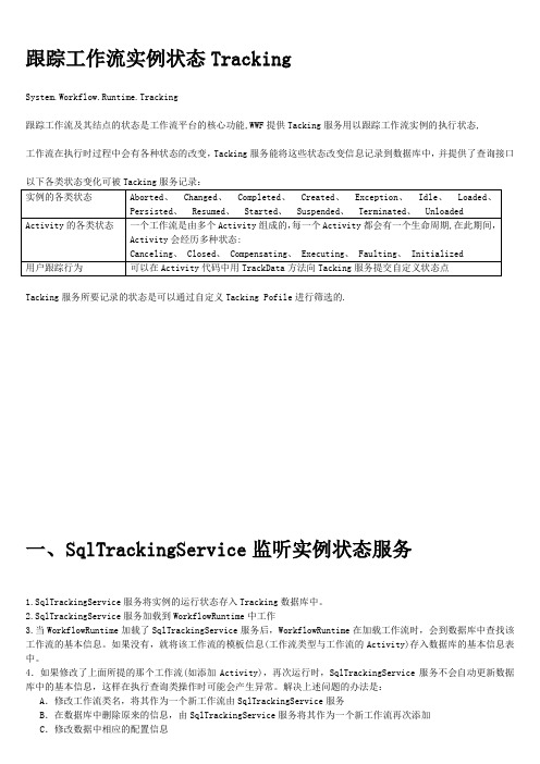
跟踪工作流实例状态TrackingSystem.Workflow.Runtime.Tracking跟踪工作流及其结点的状态是工作流平台的核心功能,WWF提供Tacking服务用以跟踪工作流实例的执行状态,工作流在执行时过程中会有各种状态的改变，Tacking服务能将这些状态改变信息记录到数据库中，并提供了查询接口Tacking服务所要记录的状态是可以通过自定义Tacking Pofile进行筛选的.一、SqlTrackingService监听实例状态服务1.SqlTrackingService服务将实例的运行状态存入Tracking数据库中。

2.SqlTrackingService服务加载到WorkflowRuntime中工作3.当WorkflowRuntime加载了SqlTrackingService服务后，WorkflowRuntime在加载工作流时，会到数据库中查找该工作流的基本信息。

如果没有，就将该工作流的模板信息(工作流类型与工作流的Activity)存入数据库的基本信息表中。

4．如果修改了上面所提的那个工作流(如添加Activity)，再次运行时，SqlTrackingService服务不会自动更新数据库中的基本信息，这样在执行查询类操作时可能会产生异常。

解决上述问题的办法是：A．修改工作流类名，将其作为一个新工作流由SqlTrackingService服务B．在数据库中删除原来的信息，由SqlTrackingService服务将其作为一个新工作流再次添加C．修改数据中相应的配置信息1.添加服务到引擎进行跟踪在WorkflowRuntime宿主程序中2.SqlTrackingQuery状态查询类SqlTrackingWorkflowInstance被查询对象类1.通过SqlTrackingQuery的TryGetWorkflow方法得到SqlTrackingWorkflowInstance对象2.通过SqlTrackingWorkflowInstance对象的属性与集合访问各类具体信息无须在WorkflowRuntime宿主程序中属性集合方法WorkflowTrackingRecord 实例状态类WorkFlow状态对象WorkflowTrackingRecord以集合成员的方式存于SqlTrackingWorkflowInstance的WorkflowEvents 集合中无须在WorkflowRuntime宿主程序中属性EventArgs实例[挂起、终止、异常]的具体信息由WorkflowTrackingRecord.EventArgs返回TrackingWorkflowSuspendedEventArgs ：挂起TrackingWorkflowTerminatedEventArgs：终止（异常就是引起终止的原因之一）TrackingWorkflowExceptionEventArgs：异常等TrackingWorkflow______Args对象，通过数据类型转换后可得到挂起 / 终止 / 异常的具体信息ActivityTrackingRecord结点状态类Activity状态对象ActivityTrackingRecord以集合成员的方式存于SqlTrackingWorkflowInstance的ActivityEvents 集合中WorkflowRuntime属性UserTrackingRecord业务状态类业务状态对象:UserTrackingRecord以集合成员的方式存于SqlTrackingWorkflowInstance的UserEvents集合中业务状态如何添加见[在Activty中向Tracking添加业务状态]WorkflowRuntime属性RuleActionTrackingEvent策略集中的策略状态(Policy节点)Workflow.Activities.Rules.RuleActionTrackingEvent具体见自定义Tracking的该部分二、自定义Tracking服务WWF提供一个tracking基本结构，可以使用他跟踪去实例改变的数据与状态,在加载项里,他提供了可伸缩性去建立更多跟踪服务应用，为一些用户的商业应用自写义tracking服务，需要实现TrackingChannel 与TrackingServic这两个类，TrackingChannel接收引擎发送的各种tracking记录,TrackingServic服务为引擎提供了接口The tracking service provides the runtime with tracking profiles based on specific parameters and conditions. It is also responsible for providing a tracking channel that receives the data sent by the runtime.引擎调用tracking服务是同步的，工作流实例执行一个阻塞直到从tracking服务有方法返回TrackingChannel实现TrackingService实现高级说明TrackingParameters类引擎将实例以[TrackingParameters类]形式传给[自定义跟踪服务TrackingService],[自定义跟踪服务]再传给[自定义Tracking通道]以[通道]在向外抛数据时可以使用传进来的该对象得到一些实例信息属性三、自定义筛选Tacking Pofile1.Tacking服务所要记录的状态是可以通过自定义Tacking Pofile进行筛选的.2.默认Tacking服务对 [实例的各类状态]、[Activity的各类状态]、[用户跟踪行为]的所有状态进行记录，可以自定义自定义Tacking Pofile让Tacking服务只记录实际需要的状态.以下各类状态变化可被Tacking服务记录,也可用Tacking Pofile进行筛选：3.自定义Tacking Pofile将生成一个XML串,存入TrackingProfile表的TrackingProfileXml字段中4.默认的Tacking Pofile以一个XML串的形式存于DefaultTrackingProfile表的TrackingProfileXml字段中5.自定义Tacking Pofile只对指定的工作流有效，默认的Tacking Pofile对所有没有自定义Tacking Pofile的工作流有效。

5g trackingareacode的值域

5g trackingareacode的值域5G的跟踪区域码（Tracking Area Code，TAC）是一个标识符，用于确定设备所在的跟踪区域。

它在5G网络中具有至关重要的作用，用于管理移动设备的位置信息以及进行网络切换。

跟踪区域码的取值范围是由国际电信联盟（ITU）和各国电信管理机构定义的。

下面将对5G 跟踪区域码的值域进行详细的阐述。

根据国际电信联盟（ITU）的规定，5G跟踪区域码是一个28位的二进制编码，可以表示的取值范围是从0到268,435,455。

这个取值范围非常大，可以满足大规模的移动设备接入需求。

每个跟踪区域码对应一个跟踪区域，跟踪区域是一个由一个或多个小区（Cell）组成的区域，用于提供无线网络覆盖。

5G跟踪区域码的编码规则和分配方式由各国电信管理机构负责管理。

根据ITU的建议，跟踪区域码的分配应该遵循一定的原则，包括避免跟踪区域码之间的重复、保证跟踪区域码的唯一性、分配合理的空间和时间资源等。

各国电信管理机构通常会根据地理位置、人口密度等因素来划分跟踪区域，并为每个跟踪区域分配一个唯一的跟踪区域码。

在5G网络中，跟踪区域码的取值决定了设备所属的跟踪区域。

移动设备在连接到网络后，会被分配一个跟踪区域码，并根据该码值进行网络切换和位置更新。

当设备进入一个新的跟踪区域时，它会向网络发送位置更新请求，网络会根据设备所在的跟踪区域码来确定其位置，并作出相应的调度决策。

跟踪区域码的值域在5G网络中扮演着重要的角色。

它不仅仅是标识设备所在跟踪区域的一个数字，还可以用于设备的位置管理、网络资源调度、信令传输等方面。

跟踪区域码的取值范围足够大，可以满足未来大规模设备接入的需求，同时也为网络规划和优化提供了灵活性。

总之，5G跟踪区域码的取值范围是从0到268,435,455，根据各国电信管理机构的规定进行分配和管理。

这个范围的大小可以满足大规模设备接入的需求，并为网络提供可靠的位置信息和调度能力。

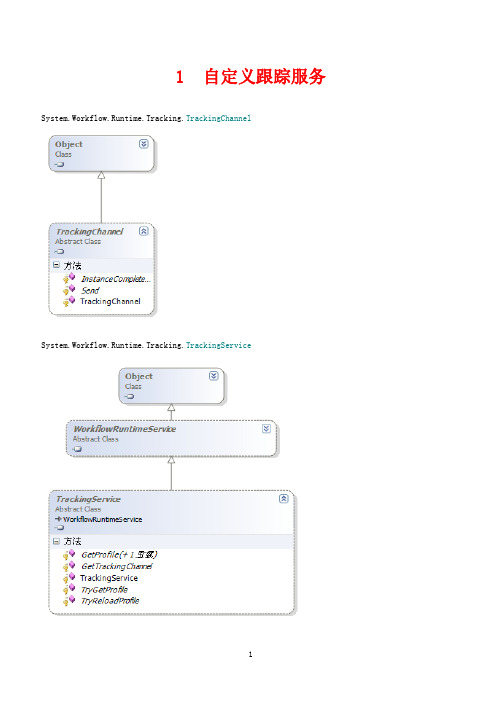
TrackingService 、TrackingChannel 自定义跟踪服务

Console.WriteLine("时间: "+ obj3.EventDateTime.ToString());
//筛选业务状态点(用户状态点)中的规则
if(erDataisSystem.Workflow.Activities.Rules.RuleActionTrackingEvent)
3．TrackingChannel接收引擎发送的各种tracking记录,
4．TrackingServic为引擎提供了接口
5．引擎调用tracking服务是同步的，工作流实例执行一个阻塞直到从tracking服务有方法返回
6．WF的工作流引擎是个黑箱子，所有有关工作流实例运行的情况或事件只有WF引擎知道，Hosting如果想知道，那么需要一个查询的界面。Tracking就是这个查询界面
{RuleActionTrackingEventobj3_rule = (RuleActionTrackingEvent)erData;
Console.WriteLine("规则名: "+ obj3_rule.RuleName.ToString());
//Policy绑定的规则集中的每个规则都会发送一组状态，Policy有点像职责链，具体以后讲
//Policy规则是自动将信息抛出的,但在类型上算上用户状态
}
}
}
}
}
//筛选结点
if(recordisActivityTrackingRecord)
{
ActivityTrackingRecordobj2 = (ActivityTrackingRecord)record;
Console.WriteLine("时间: "+ obj2.EventDateTime.ToString());

Tracking_Urbanization

36FEBRUARY · 2O13PEOPLEText by Zhang HongWang Jun is a journalist who has worked with Xinhua News Agency for more than two decades.Wang began working at the Beijing-based news agency upon graduating from col-lege in 1991 when China was experiencing its fastest and most massive urbanization in history.In Wang’s computer is one of his trea-sures – an old picture of Beijing City taken from atop the White Pagoda in Beihai Park in 1912.“What a beautiful city!” every time he looks at the image his pulse races. “More than a million people were making a living there, yet it was fundamentally a forest. Ev-ery courtyard had trees, and from that high point the city looked like a sea of green. The blue-bricked and grey-tiled courtyard houses were hidden beneath the greencanopy.” Wang was reminded of what I. M. Pei said when the Chinese-American archi-tect first climbed Jingshan Hill in Beijing: “I am Chinese.”Bulldozers’ ForceOn July 13, 2001, Beijing won the bid to host the 2008 Olympic Games. After witnessing the jubilant celebration on Chang’an Avenue late that night, Wang was filled with peaceful wishes as well as worry for the city. On his way backTracking UrbanizationJournalist Wang Jun and His Contemplation of Beijinghome from work, he noticed that Tu’er and Xiang’er hutong s (traditional alleyways), from the 13th and mid-14th centuries re-spectively, had disappeared without a trace. That same year, permanent residents of the city passed 20 million, and the former residence of well-known 20th-Century architectural historian, architect, cityplanner, and educator Liang Sicheng (1901-1972), and his wife, architect and poet Lin Huiyin (1904-1955), was razed. Statistics of China’s third national cultural heritage census showed that 969 unmovable cultural relics had vanished.After Beijing’s successful bid for the 2008 Olympics, 280 billion yuan was earmarked for preparations. “We were so moved after hearing the news,” Wang recalls, “because it meant that the door of the country would remain irreversibly open. It was an honorable event, but at the same time we worried what the city would become after the large investment was spent.” All his worries and thoughts on the problem later inspired his bestselling Bei-jing Record, a Physical and Political History of Planning Modern Beijing .Since the 1950s, the capital city started expanding outward from a single center point so vividly that it has been compared to “making a pancake from the center out.” “The trend of radiation from a single center structure will emphasize focus on the development of infrastructure in the central area, which will create consider-able construction work in the central area,” Wang explains. “The present central area of Beijing evolved from what it was in the Yuan (1271-1368), Ming (1368-1644) andQing (1644-1911) dynasties. In 1949, it was already home to 1.3 million residents and was already covered with buildings. So, adding so many more buildings in an already crowded central area inevitably leads to pulling down old ones, large-scale relocation of residents, and ultimately daily commuting problems.”“Beijing’s traffic problem can be largely attributed to excessive concentra-tion of city employment functions around the Forbidden City,” Wang continues. “Now, the suburban area is for sleeping. For example, Wangjing, Tiantongyuan and several other peripheral residential quarters accommodate several hundred thousand people. So, every day hundreds of thou-sands of people travel to the city for work in the morning and return home to the suburbs in the evening.”Wang contends that even if it had been a spacious area without established urban districts and the Forbidden City, the one-centered structure plan was terrible for a city that would accommodate a population of 10 million, never mind one with so much priceless heritage in its central area.A Tsinghua University professor even once revealed to Wang that some people had proposed removing the For-bidden City.Astonished and shocked, Wang tracked down and interviewed the architect respon-sible for the removal project and read the files he could find. Everything he heard and saw confirmed the professor’s revelation. “Beijing made two plans to remove the old city in the past.’’ Wang notes. “One was in 1990, and it aimed to renovate the dilapi-Copyright ©博看网. All Rights Reserved.The siheyuan (quadrangle with rooms arrangedon four sides of a courtyard) is a traditionalChinese dwelling style. In old Beijing, the blue-bricked and gray-tiled siheyuans were clusteredtogether creating a unique scene. Pictured are si-heyuans near Nanluoguo Lane that were addedto the protection list of the city in 1987. Xinhua Copyright©博看网. All Rights Reserved.38FEBRUARY ·2O134 Beidaji Lane in Dajipian traditional hutong area, Xicheng District, Beijing. Left: A child plays in front of a quadrangle on February 22, 2007. Right: The same site on April 3, 2012. CFPCopyright ©博看网. All Rights Reserved.dated old houses in ten years. The other was made in 2000 with the goal to renovate dilapidated houses in five years. Today, probably less than a third of the old urban district remains.”Construction of a Multicenter City with Balanced Development In the first quarter of 2011, subway passengers surpassed 400 million in Bei-jing, a phenomenon jokingly described by netizens as “people in but flat pictures out; biscuits in but flour out.”“This is the consequence of past plan-ning,” Wang sighs, visibly pained every time he mentions the removal of old dis-tricts. “We feel the pain Mr. Liang Sicheng experienced.”Wang is a firm supporter of Liang, who dedicated himself to preserving the country’s ancient buildings and cultural relics his entire life. In spite of his efforts to preserve the old capital, the former city gates and city walls were torn down in the 1950s. Wang highly praises Liang’s ideas on urban planning: A large municipal-ity should be divided into several small districts that resemble cells, separated by green belts. When one cell is full, a new one should be built.“I became very excited when I first read Liang’s plan,” Wang grins. “He answered the exact question I had been pondering: How to free the city from traffic congestion. This is a plan for the future.”“His plan not only focused on the protection of the old town,” Wang adds. “It also pointed out that placing the ad-ministrative area near the Forbidden City would cause a great number of people to move outside the city, and eventually these people would have to travel all the way to the old town for work. This is the main culprit for the traffic problem.”But ironically, even Liang’s former resi-dence was a victim of the “removal storm.”In the 1930s, Liang documented theimportant city walls and city gates in Bei-jing with his camera and even conductedsurveying and mapping work. “It is reallypainful,” Wang sighs as he examines thosemaps now at Tsinghua University. “Just ashis work was completed, Japan launchedwar against China. Liang and his wife wereforced to leave Beijing, and never got thechance to publish his survey of Beijing’scity walls.”Wang and his colleague Liu Jiangconducted a joint survey on the municipaldevelopment model of Beijing, trying todetermine whether Beijing’s layout couldpossibly meet the requirements for expan-sion for the 2008 Olympics.The survey attracted major attentionfrom decision-makers and triggered amassive project to edit and revise Beijing’soverall plan. In January 2005, Beijing CityMaster Plan (2004-2005) was approvedby the State Council. The plan includedcomprehensive preservation of the old city,reinforced development of new urban dis-tricts, and adjustments of urban structuresas its strategic goals.Wang is excited that the latest masterplan for Beijing has finally returned to theblueprint of Liang and Chen Zhanxiang(1916-2001), another city planning expertwho also pushed an idea in the 1950s thathas not yet been realized: to construct acity with several centers and balanceddevelopment.Wang attributes Beijing’s traffic con-gestion problem to the improper layout ofthe city and related strategy. “We live in ahighly dense society excessively dependenton car transportation,” Wang opines. “About30 percent of the residents travel by car,another 30 percent by the means of publictransit and the rest by bicycle or on foot.Beijing has been developing various trans-portation modes equally, and the result isthat all modes have encountered trouble.”However, Wang rejoices that overthe past decade the public has been moreinvolved in protecting Beijing’s culturalrelics, and that related government sectorshave begun realizing that listening and co-operation are crucial to better preservation.“The city has already mapped out amaster plan for comprehensive preservationof the old city,” Wang stresses. “It requiresthe unremitting efforts of every citizen wholoves his or her hometown.”Outlook Beijing, City Docu-mentation, and A Decade into the Urban Century. The New York Review compared Beijing Record to Jane Jacobs’ , a classicurban conservation.About Wang JunCopyright©博看网. All Rights Reserved.39C H I N A P I C T O R I A L。

国际包裹查询轨迹中英文对照

国际包裹查询轨迹中英文对照国际包裹查询轨迹中英文对照进口海关查验被取消Import customsinspection canceled货物电子信息已经收到Shipment information receivedUselessUseless正在操作订单Orders are being processed操作完成Shipment operation completed已经在派送途中Out for delivery已在派送途中-至偏远地区Out for delivery -To beyond point 货物已经派送Shipment delivered货物已签收-收件人自提Shipment delivered-Consignee collection货物已经派送--手机短信返回PODShipment delivered-Pod return by GSM short message邮件已派送parcel has been delivered货物已经派送--转邮政派送Shipment delivered-Forwarded to post office 邮件已投寄parcel posted收货人已签收Shipment delivered-Signature by consignee货物已经派送并签收-收件人口头确认收到货件Shipmentdelivered-VerbalPODconfirmation from recipient 订单已经出库Orders have been out of warehouse邮件到达中转站parcel arrived at exchange office部份货物己经签收Partial Delivery邮件离开中转站parcel departed from exchange office邮件中转parcel dispatched from original office邮件投寄收件局parcel forwarded to Post Office已收到电子信息Parcel information received作业中心内部操作Process at Location邮件被退回-地址不详parcel returned-Insufficient address邮件被退回-查无此人parcel returned-Receiver not found邮件被退回-收件人拒收parcel returned-Receiver refused邮件被退回parcel returned邮件被退回-无人认领parcel returned-Unclaimed邮件操作parcel scanned and Processed投递Posted货物已从发件人处提取Shipment picked up邮件已提取parcel was picked up海关已经放行Released from customs海关放行被取消Release from customs canceled收件人拒收货物Receipients refused to accept shipment货物已退回发件地Returned to shipper货物破损Shipment damaged货物再次中转Shipment departed from facility again货物暂扣Shipment on hold货件暂扣-等待收件人提供资料Shipment on hold-Awaiting paperwork货件暂扣-等待确认偏远费用Shipment on hold-Need recipient conform ODA chargeTrackingmore国际包裹查询货物暂扣-收件人关税未付Shipment on hold-Duty not pay货物暂扣-收件人没有准备好费用Shipment on hold-Payment not ready货物暂扣-超出服务派送范围SHIPMENT ON HOLD-OUT OF DELIVERY AREA货件暂扣-等待费用到帐Shipment on hold-Payment deposited 货物暂扣-由于收件人拒付到付费用Shipment on hold-Refuse pay COD charge 货物暂扣-收件人拒付关税Shipment on hold-Consignee refused to pay duty货件暂扣-由于收件人拒绝支付费用SHIPMENT ON HOLD-REFUSE TO PAY CHARGE货物暂扣-需要提供入仓单，并确认入仓费用SHIPMENTONHOLD-WAREHOUSEDOCANDCHARGE CONFIRMATION NEEDED货件暂扣-由于重量不符Shipment on hold-Due to weight difference根据发件人要求退回货物Return as shipper's request货物从海关退回公司Shipment returned from customs to facility货物在转运中Shipment in transit货件转运-由当地邮政安排中转派送SHIPMENT IN TRANSIT-DELIVERED BY THE POST OFFICE货件转运-交机场SHIPMENT IN TRANSIT-TO THE AIRLINE货件转运-中转到清关点Shipment in transit-To the customs货件转运-转往目的地Shipment in transit-To the destination city货件转运-航空公司卸载Shipment in transit-Consignment unloaded from the airline转运延迟Transport delay转运延迟-等待转交代理Transport delay-Awaiting collection from agents转运延迟-由于恶劣天气Transport delay-Due to bad weather 转运延迟-由于目的地机场被封锁Transport delay-Due to destination airport was blocked转运延迟-由于航班取消导致延迟Transport delay-A flight was canceled and caused delay由于航班取消导致转运延迟被取消Transportdelaycanceled-Aflightwascanceledandcaused delay转运延迟-航班晚点Transport delay-Flight delayed转运延迟-由于机械故障导致航班延迟Transportdelay-Aflightdelayoccurredduetomechanical reasons转运延迟-由于货件中存在违规危险品Transport delay-A hazardous material irregularity hasoccurred with the shipment转运延迟-当地假期Transport delay-Due to local holidays转运延迟-交货晚点，无法赶上航班Transport delay-Late arrival and miss the flight转运延迟-未提到货物，航空公司调查中TRANSPORTDELAY-CONSIGNMENTNOTFOUND,AIRLINE START INVESTIGATING转运延迟-由于航空公司卸货延迟Transport delay-The airline off-loaded Shipments causingdelay转运延迟-其他省市Transport delay-T o other provinces转运延迟-由于公共假期Transport delay-Due to public holiday 转运延迟-特殊地区TRANSPORT DELAY-TO SPECIAL AREAS转运延迟-由于正在接受安全检查Transport delay-Due to security check转运延迟-等待航班Transport delay-Wait for the flight邮件深查中Under Investigation货物等待中转Wait Transport货物等待中转被取消Wait transport canceledTrackingmore国际包裹查询货物到达港口Shipment arrived at airport货物到港被去消Shipment arrived at airport canceled货物到达作业中心Shipment arrived at facility货物到达作业中心被取消Shipment arrived atfacility canceled 根据客户要求，快件正等候收件人自取Awaiting pick up by recipient as requested结案Case closed发件人自提Shipment fetch by shipper货物交由收件人的清关代理清关Handed over to recipient broker for clearance货物已经遗失Shipment missing货物交由第三方代理派送，无派送结果Delivery arranged,no signature expected收件人自己安排清关，文件已派给收件人PAPERWORKHANDEDOVERTORECIPIENTBROKER FOR CLEARANCE货物交由第三方代理退回至发件人Delivery arranged,return to shipper海关扣件-快件被海关没收HELD IN CUSTOMS-CONSIGNMENT SEIZED BY CUSTOMS货物已经被销毁Shipment destroy 货物在清关Customs clearance in progress海关退关Customs return请联络4PXPlease contact 4PX货物离开起运港Shipment departed from airport货物离港被取消Shipment departed from airport canceled货物件到达目的地Shipmnet arrived at destination country派送延迟Delivery delay派送延迟-等待收件人回复Delivery delay-Awaiting reply from recipient派送延迟-无收件人电话或收件人电话无人接听Deliverydelay-Telephonenorespondorbad number派送延迟-天气恶劣Delivery delay-Due to bad weather派送延迟-收件人要求更改地址Delivery delay-Consignee request to change the address派送延迟-正在联系收件人Delivery delay-Countacting Consignee...派送延迟-收件人搬离派送地址Delivery delay-consignee moved派送延迟-需要收件人的信息Delivery delay-consignee not available派送延迟-派送关门Delivery delay-Company closed派送延迟-收件人地址不正确或不完整Delivery delay-Incorrect/incomplete address派送延迟-错过派送时间Delivery delay-Missed delivery cycle派送延迟-由于错误分拣Delivery delay-Due to missort派送延迟-货物不在当地，查找中Deliverydelay-Consignmentnotfound,investigationstarted派送延迟-收件人不在当地Delivery delay-Consignee not in the country派送延迟-收件人在休假Delivery delay-Recipients on holiday 货件暂扣-已通知收件人Shipment on hold-Recipient contacted派送延迟-派送时收件人不在Delivery delay-Recipient not at home派送延迟-收件人要求约时间派送Deliverydelay-Recipientsrequesttoholdforfuturedelivery date派送延迟-到达错误目的地正转往正确目的地Deliverydelay-Baddestinationandresendtoright destinationTrackingmore国际包裹查询派送延迟-已联络发件人Delivery delay-Shipper contacted派送延迟-由于罢工或骚乱Delivery delay-Due to strike / riots 派送延迟-货物不在当地，仍在查找DELIVERYDELAY-CONSIGNMENTNOTFOUND,KEEPSEARCHING派送延迟-由于交通问题Delivery delay-Due to traffic problems 货物离开作业中心Shipment departed from facility货物离开作业中心被取消Shipment departed from facility canceled计划安排派送Scheduled for delivery已经安排派送-偏远地区转第三方派送Scheduledfordelivery-Remotearea,deliverybythird party销毁货物the shipment has been destroyed销毁货物-由于客户要求the shipment has been destroyed as request销毁货物-由于涉嫌商标侵权the shipment has been destroyed due to tradmark出口海关查验Export customs inspection 出口海关查验被取消Export customs inspection canceled海关扣件Held in customs海关扣件-正在评估关税Held in customs-Custom appraising the duty and tax 海关扣件-等待海关通知Held in customs-Awaiting information from Customs海关扣件-等待收件人提供清关资料Heldincustoms-AwaitingclearancepaperworkfromRecipient海关扣件-由于海关计算机系统宕机Heldincustoms-Duetocustomscomputersystembreakdown海关扣件-收件人在联系海关处理相关事宜custom directly to handleHeldincustoms-Recipientwillcontactthe海关扣件-收件人确认关税Held in customs-Recipient confirm to pay for the duty and tax海关扣件-正在等待收件人的清关资料Heldincustoms-Awaitingclearancefilefromconsignee海关扣件-需要收件人信息Held in customs-Need consignee's information海关扣件-海关不接受提供的资料Held in customs-Paperworks rejected by customs海关扣件-由于报关数据未提供Held in customs-Due to data not available海关扣件-要求正式进口报关Held in customs-for formal entry submission海关扣件-需要收件人确认关税Held in customs-Need recipient confirm duty and tax海关扣件-由于活体动物进口Held in customs-Due to live animal entry海关扣件-收件人没有回应Held in customs-No response from recipient海关扣件-需要收件人授权Held in customs-Need consignee authority海关扣件-产生罚款Held in customs-Fine & penalty imposed from customs海关扣件-等候检查检疫Held in customs-Pending inspectionand quarantine海关扣件-等候海关放行Held in customs-Pending customs released海关扣件-需要清关文件Held in customs-Need paperwork已确认收货Has confirmed receipt海关扣件-收件人要求自己清关，等待确认Heldincustoms-Recipientwillarrangeclearance, awaiting confirmation 海关扣件-收件人拒绝协助清关Held in customs-Recipient refuse to provide instruction海关扣件-由于安全检查Held in customs - Due to security checkTrackingmore国际包裹查询海关扣件-需要有效税号Held in customs-Need a valid tax identification number海关扣件-敏感货物Held in customs-Unacceptable goods海关扣件-由于检查商品描述Held in customs-for verify commodity description 海关扣件-由于检查商品价值描述Held in customs-for verify value description 海关扣件-由于物品申报不符Held in customs-Wrong commodity declaration海关扣件-等候收件人清关指示Heldincustoms-Awaitingclearanceinstructionsfromconsignee海关扣件-由于价值申报不符Held in customs-Wrong value declaration作业中心扣件Held in facility作业中心扣件-由于付款未到Held in facility-Due to payment not readyTrackingmore国际包裹查询。

tracking.js的使用方法

tracking.js的使用方法tracking.js 是一个开源的JavaScript 库，用于在现代浏览器中进行实时的计算机视觉任务。

它通过使用计算机视觉和机器学习技术，提供了一种简单的方法来检测和跟踪人脸、人眼、人体、手势、颜色等对象，以及进行图像滤镜和图像分割等任务。

本文将介绍tracking.js 的基本使用方法，包括安装、初始化、跟踪和检测等步骤。

第一步：安装tracking.js要使用tracking.js，首先需要将其添加到你的项目中。

你可以通过使用npm 或yarn 来安装它，也可以直接引入它的CDN 链接。

下面是两种不同的安装方法：使用npm 或yarn 安装：npm install tracking或yarn add tracking使用CDN 引入：在HTML 文件的头部中添加以下代码：<script src="第二步：初始化Tracking.js当你已经安装好tracking.js 后，就可以在你的项目中初始化它。

首先，在HTML 文件的头部或脚本文件中引入tracking.js 库，例如：<script src="path/to/tracking.js"></script>或import * as tracking from 'tracking';然后，在你的JavaScript 代码中初始化tracking.js：var video = document.getElementById('video');tracking.track(video, tracker);这里的`video` 是你的视频元素，`tracker` 是用于追踪特定对象的跟踪器。

第三步：创建跟踪器在tracking.js 中，跟踪器是用来追踪特定对象的实例。

跟踪器可以跟踪不同类型的对象，包括人脸、人眼、人体、手势或颜色等。

Oracle Asset Tracking 产品说明书

Oracle Asset Tracking Oracle Asset Lifecycle Management SolutionO R AC L E AS S E T T R AC K I N GK E Y B U S I N E S S B E N E F I T S•Improve asset visibility, tracking, and control with a single global asset repository•Streamline and automate Asset creation and update operations •Manage end-to-end “Procure to Retire” process and efficiently conduct asset deployment transactions such as move, reinstatement, and deployment transactions•Automatically synchronize the operational and physical events of assets with the financial updates in Oracle Fixed Assets•Improve maintenance of assets through integration with Oracle Enterprise Asset Management and Oracle Field ServiceK E Y F E A T U R E S•Single global repository of asset information•Comprehensive view of assets and configurations•Streamlined Asset Creation and Updates to Assets to accurately manage physical asset and financial asset information•Conduit between inventory, Purchasing, and Fixed Asset to automatically create assets and update records in multiple modules. Changes to assets captured with inputs from over 85 E-Business suite transactions Capital-intensive companies face many challenges while managing assets such as dealing with a large volume of data associated with these assets, tracking and maintenance of assets, and need for accurate financial reporting. Oracle® Asset Tracking is a comprehensive asset lifecycle tracking application that provides tracking, visibility, and control of globally dispersed assets for capital-intensive companies, along with complete transaction auditing. Asset deployment transactions such as install, in-service, out of service, or asset moves can be completed efficiently. Through integration with Oracle Assets, the financial impact of these physical asset transactions can be easily managed, thereby significantly reducing the amount of manual intervention required to maintain financial accuracy along with physical tracking. This enterprise-wide integration helps achieve a single source of truth for enterprise assets while reducing the total cost of ownership.Figure 1: Comprehensive asset tracking, management, and financial reporting Improve Asset Visibility, Tracking and Control with a Global Single Asset RepositoryAsset lifecycle tracking has become an increasingly important issue for organizations with a large asset base. The lack of visibility and accurate and timely updates of assets leads to unnecessary purchases of equipment, high asset carrying costs, and excessive regulatory fines. It is imperative for capital-intensive companies to know the exactnumber of the existing assets, their current value, and location and maintenance history.•Unlimited versioning of Assets •Mass updates of assets•Easy multiple-asset deployment •Complete tracking of asset history •Automatic fixed asset creation in Oracle Assets upon receipt or after asset is moved to in-service•Automatic handling of costs, units, and location updates in Oracle Fixed Assets for transactions such as inventory transfers, asset deployments or redeployments, and internal sales order shipments •Supports asset transfers between internal organizations•Supports Management of Replacement /Loaner/ Customer Site Located Assets•Facilitates capitalization into Fixed Assets for depreciation and accurate asset valuation•Supports Capitalize on Issue (COI) business process•Support Serialized asset grouping for capitalization•Support Vintage pooling functionality for non-serialized items•Support for depreciating asset inventory•Support for managing cost deviations such as Invoice price adjustments •Support for asset re-classification scenarios•Support for direct project receipt •Support for Project expenditure reversal for deployed asset’s move to inventory•Access to maintenance information Without this vital information, it is challenging to properly plan, procure or construct and deploy assets, or perform maintenance activities.Oracle Asset Tracking integrates with Oracle's other operational and financial products such as Oracle Inventory, Oracle Projects, Oracle Assets, and Oracle Enterprise Asset Management to offer a comprehensive, reliable, and efficient asset lifecycle tracking application, along with complete transaction auditing.It provides a comprehensive view of assets and their configurations, regardless of whether the assets are at a field location or within a warehouse. A wide range of physical information such as the quantity, serial number, location, usage, counter reading of the equipment, and deployment order details is tracked. It also manages information about the asset inter-relationships and provides a graphical visualization of these relationships, thus enhancing user experience.On the financial side, integration with Oracle Assets allows the tracking of the financial fixed asset details. Integration with Oracle Enterprise Asset Management and Oracle Field Service provides easy access to maintenance and service history of the assets.Streamline Asset Creation and Updates to AssetsOracle Asset Tracking increases efficiency by drastically reducing the need for manual intervention in the asse t creation process. Capitalizing on Oracle Asset Tracking’s tight integration with Oracle Assets, as an asset is received and delivered to the enterprise, the corresponding financial asset is automatically created. Cost deviations, such as invoice variances, can be easily captured and communicated back to Oracle Assets, providing accurate and comprehensive asset financial information.Any financial fixed asset created directly in Oracle Assets triggers a notification for the creation of the physical asset in Oracle Asset Tracking. The users can either manually create a new asset, or copy an existing asset, or simply select an existing asset to link it with the fixed asset. To efficiently support large global rollouts for management of physical and fixed assets, Oracle Asset Tracking supports multiple Fixed Asset (FA) Book Types.The seamless synchronization of Oracle Assets and Asset Tracking ensures that an asset’s location and status are up-to-date and accurate. Summary data of physical assets can then be reconciled to the detailed asset data for financial and tax reporting.Through the integration with other E-Business Suite modules, Oracle Asset Tracking maintains the history of asset transactions that occur in other modules, such as Procurement, Order Management/ Shipping, Projects, Field Service, and Enterprise Asset Management.Manage end-to-end “Procure to R etire” processOracle Asset Tracking allows companies to manage the “Procure to R etire” process end-to-end and efficiently conduct asset deployment transactions such as move, reinstatement, retire and other deployment transactions.O R A C L E A S S E T T R A C K I N GR E L A T E D P R O D U C T SOracle Asset Tracking is complemented by the following products for end-to-end asset tracking across the enterprise:•Oracle Assets•Oracle Enterprise Asset Management•Oracle Field Service•Oracle Install Base•Oracle Inventory•Oracle Purchasing•Oracle Projects•Oracle ServiceR E L A T E D S E R V I C E SThe following services support Oracle Asset Tracking:•Update Subscription Services •Product Support Services •Professional Services•Oracle E-Business Suite Accelerators •Oracle Application Solution Centers •Oracle University•Oracle Consulting Figure 2: End-to-end asset visibility, tracking, and controlEasy Asset Deployment TransactionsOracle Asset Tracking support the following asset transactions:•Install•Move•Project Transfer•Put into Service•Retirement•Take out of Service•Un-InstallWith a single transaction, the users can easily deploy a single, specific asset or multiple assets at different locations with full or partial quantities, making asset deployment transactions easy and transparent. The comprehensive availability of physical and financial information improves decision making during asset planning and deployment, helping to reduce asset obsolescence and unnecessary purchases.Asset Deployment With or Without Oracle ProjectsThe integration between Oracle Asset Tracking and Oracle Projects allows assets to be issued to a Capital Resource Logistics (CRL) project prior to deployment. Prior to deployment, assets can also be transferred between projects. The expenditure items will be reversed in the origin project, and added to the destination project. The assets can also be deployed in service at field locations directly from inventory without first being issued to CRL projects. The assets can be brought back to a warehouse and issued to another location. Throughout all these asset movement, the link to Oracle Fixed Assets is maintained. Tracking valuable assets and deploying them for the best possible use improve efficiencies and return on investment.Asset Transfers between Internal OrganizationsOracle Asset Tracking supports all asset transfers between internal organizations. Assets can be moved by various operational transactions such as inter-organization transfer and internal sales order transfer. The Oracle Asset Tracking background process supports all asset updates for the source and destination organizations. This feature may be used to plan and track a complicated network construction project bydesignating the build site as a project in one organization that drives resource demands to the main inventory organization.Management of Replacement /Loaner AssetsAn asset can be shipped to a customer as a sale or a loaner as a temporary replacement for a repaired asset. Other business requirements may necessitate an enterprise asset to be located at a customer’s site. Oracle Asset Tracking and Oracle Order Management help track these assets by supporting transaction subtypes which indicate whether there is a change in ownership. An asset sales or location change will be initiated accordingly for Oracle Assets.Support Capitalize on Issue (COI) business processThis feature enables customers to perform Capitalize on Issue (COI) business process using sales order shipment flow. It provides efficient management of Operating Lease process followed by Equipment Rental and Leasing firms and facilitates seamless flow of Asset Clearing Account and Date Placed in Service (DPIS) details to Fixed Asset book.Improve Asset MaintenanceMaintenance operations are an integral part of an asset’s lifecycle management. An asset’s maintenance history is necessary for efficie nt asset management. A single global Asset Repository architecture enables an asset to be simultaneously tracked by Oracle Asset Tracking and maintained/ serviced by Oracle Enterprise Asset Management/ Oracle Field Service. A user can easily access details about the maintenance work history of an asset through work requests/ work orders and service requests.Oracle Asset Tracking Command CenterThe Oracle Asset Tracking Command Center enables efficient capitalization and improved tracking of item instances which are eligible for fixed asset creation through Oracle Asset Tracking. The Capitalization dashboard contains actionable insights on transactions and instances that are pending in various stages of capitalization process. This dashboard provides a rich set of components to allow browsing, drilling down to details, interactive search and analytical capabilities using available refinements, charts, graphs, tag cloud and results tables. Through this "information-driven navigation", users can drill down to specific records and follow guidance on next steps to progress on fixed asset creation for acquired assets in a seamless flow.The Oracle Asset Tracking Command Center is available at no additional cost to licensed users of Oracle Asset Tracking, Release 12.2.4 and above.Figure 3: Oracle Asset Tracking Command CenterOracle® Asset Tracking is a comprehensive asset lifecycle trackingapplication that provides tracking, visibility, and control of globally dispersedassets for capital-intensive companies, along with complete transactionauditing. It provides a comprehensive view of both financial and operationalinformation, which forms the foundation for Asset Lifecycle Management.C O N T A C T U SFor more information about Oracle Asset Tracking, visit or call +1.800.ORACLE1 to speak toan Oracle representative.C O N N E C T W I T H U S/oracle/oracle/oracleCopyright © 2015, Oracle and/or its affiliates. All rights reserved. This document is provided for information purposes only, and thecontents hereof are subject to change without notice. This document is not warranted to be error-free, nor subject to any otherwarranties or conditions, whether expressed orally or implied in law, including implied warranties and conditions of merchantability orfitness for a particular purpose. We specifically disclaim any liability with respect to this document, and no contractual obligations areformed either directly or indirectly by this document. This document may not be reproduced or transmitted in any form or by any means,electronic or mechanical, for any purpose, without our prior written permission.Oracle and Java are registered trademarks of Oracle and/or its affiliates. Other names may be trademarks of their respective owners.Intel and Intel Xeon are trademarks or registered trademarks of Intel Corporation. All SPARC trademarks are used under license andare trademarks or registered trademarks of SPARC International, Inc. AMD, Opteron, the AMD logo, and the AMD Opteron logo aretrademarks or registered trademarks of Advanced Micro Devices. UNIX is a registered trademark of The Open Group. 0115。

FANUC 机器人 Line Tracking 线性追踪技术使用方法详解

FANUC 机器人Line Tracking 线性追踪技术使用方法详解目录：机器人技术1. 什么是线性追踪Line Tracking线性追踪也就是我们经常听到的链速追踪，主要用来处理移动工件的取放，将运动物体的速度和方向发送给机器人，机器人控制器经过算法处理后，使机器人移动速度和运动物体相同，从而保证机器人和运动物体之间相对静止，最终实现准确的取放件。

比如机器人从皮带输送机取件，使用Line Tracking后，机器人就可以在输送机不停的状态下，直接从皮带输送机上取件。

2. 线性追踪Line Tracking 功能描述线性追踪有2种实现方式：▪单轴线性追踪Single axis line tracking▪笛卡尔直线或圆环追踪Cartesian line or circular tracking2.1 单轴线性追踪Single axis line tracking主要是针对机器人附加轴的，保证机器人附加轴的运行速度和输送机相同，使用单轴线性追踪的前提必须保证输送机输送方向和机器人附加轴方向相同。

比如机器人地轨，使用单轴线性追踪后，机器人地轨的运动速度就可以和输送机相同。

2.2 笛卡尔直线或圆环追踪Cartesian line or circular tracking笛卡尔追踪指的是机器人工具中心点TCP（Tool Center Point）自动追踪输送线，笛卡尔追踪只能使用直线运动和圆运动踪两种，不能使用关节运动。

2.2.1 直线追踪笛卡尔直线追踪系统，一般由机器人、直线输送机组成，当工件从机器人前方经过时，机器人可以准确抓取工件。

2.2.2 圆弧追踪笛卡尔圆弧追踪系统，一般由机器人、圆弧形输送机或旋转工作台组成，直接可以直接从上面取放件。

圆弧追踪不支持边界设定。

3 硬件和软件线性追踪系统要求控制器带有线性追踪接口，可以连接输送机速度编码器。

注意：线性追踪作为附加选项，购买机器人的时候，需要特别指定，标准版机器人不带这个功能。

快递查询API接口（51tracking）

快递查询API接⼝（51tracking）快递查询接⼝⽬前提供快递查询的接⼝平台有：快递100快递⽹不同接⼝的区别：（1）51tracking⽀持380家快递公司，其中有55家为国内的快递，其余325家为国际快递。

具体的价格为0.8分钱/单号左右，新注册⽤户可以免费测试12⼩时。

（2）快递100属于在国内做得⽐较早的平台，可以申请每天最多2000次的API调⽤，但需要给快递100做⼀个友链。

超过2000次收费，每次0.06~0.1元不等。

（3）快递⽹可以申请每天最多500次的API调⽤，但同样需要做⼀个友链。

超过部分，每次0.05元。

快递API的应⽤场景与⽤途1. 最常见的应⽤场景如下：（1）电商⽹站：例如B2C、团购、B2B、批发分销站、C2C、本地⽣活交易等⽹站。

（2）管理系统：订单处理平台、订货平台、发货平台、分销系统、渠道管理系统、客户管理系统、ERP等。

2. 快递API的⽤途如下：（1）让顾客登录⽹站后，直接在“我的订单”页⾯内就能看到订单的物流状态。

（2）⾃动筛选出“已签收”、“疑难件”等状态的单号，减轻物流跟单⼈员的压⼒。

（3）改变订单的状态和交易流程，例如单号变为“已签收”，就能让订单变为可以确认退换货等。

（4）评估选择快递公司，根据“已签收”的运单数，可以算出销售⼈员的业绩，且便于应对货到付款的结算。

（5）邮件、短信提醒⽤户运单的最新状态，可以安抚⽤户，也可以利⽤邮件短信⼆次营销。

对接⽰例这⾥以51tracking为例，不同的接⼝的对接⽅式⽐较类似，都需要注册，并⽣成⾃⼰的API key。

以下以51tracking的查询API为例。

接⼝⽀持的消息接收⽅式为HTTP POST 请求⽅法的编码格式为 utf-8 请求body部分的参数的数据格式为json 格式接⼝参数接⼝请求地址请求头部信息参数参数名称类型说明是否必须Content-Type: application/json定义请求头部的数据格式是Trackingmore-Api-Key: string后台获取的API是请求body参数说明参数说明类型说明是否必须tracking_number string查询快递的快递单号是carrier_code string51tracking定义的快递商简码，⽐如china ems 就是china-ema是carrier_code 参数是51tracking ⾃⼰定义的快递商家的简码。

track的用法

track的用法一、track的基本用法1. 作名词- 表示“小路，小径”。

例如：We followed a muddy track through the forest.（我们沿着森林里一条泥泞的小路前行。

） - 表示“跑道”。

如：The athletes are warming up on the track.（运动员们正在跑道上热身。

）- 表示“轨道”。

例如：The train runs on the track.（火车在轨道上行驶。

）- 表示“踪迹，足迹”。

例如：The hunters found the tracks of a deer in the snow.（猎人们在雪地里发现了一头鹿的踪迹。

） - 表示“（唱片或光盘等上的）歌曲，乐曲”。

例如：I really like the last track on this album.（我很喜欢这张专辑的最后一首曲子。

）2. 作动词- 表示“跟踪，追踪”。

例如：The police tracked the suspect for days.（警察追踪那个嫌疑犯好几天了。

）- 表示“观察（进展情况）”。

例如：I'm tracking my progress in learning English.（我正在观察自己英语学习的进展情况。

）二、track的固定搭配1. keep track of- 意思是“记录；与……保持联系；了解（某人或某物的）动态”。

例如：- It's hard to keep track of all my friends' birthdays.（要记住我所有朋友的生日可真难。

）- She uses a notebook to keep track of her daily expenses.（她用一个笔记本记录自己的日常开销。

）2. lose track of- 意思是“失去与……的联系；不能跟上……的进展”。

目标跟踪系统

目标跟踪系统目标跟踪系统（Object Tracking System）是一种能够自动检测、追踪和跟踪运动目标的计算机系统。

目标跟踪系统由一个或多个传感器，例如摄像机或雷达，一个目标检测算法和一个目标跟踪算法组成。

它广泛应用于许多领域，包括视频监控、智能交通系统和无人驾驶车辆。

目标跟踪系统的核心任务是从传感器获取的输入数据中提取目标并预测它们的运动轨迹。

目标检测算法通常使用计算机视觉技术，例如模板匹配、颜色分割和特征提取，来检测输入图像中的目标。

一旦目标被检测到，目标跟踪算法将对目标进行跟踪，通过连续观察目标在每一帧中的位置，速度和加速度等信息，预测目标的未来位置。

目标跟踪系统的性能取决于目标检测和目标跟踪算法的准确性和效率。

现代目标检测算法通常基于深度学习技术，例如卷积神经网络（CNN），能够在复杂背景和遮挡的情况下准确地检测目标。

目标跟踪算法则使用过滤器或轨迹预测方法，例如卡尔曼滤波器或粒子滤波器，来估计目标的状态并跟踪目标。

目标跟踪系统还可以通过使用多个传感器来提高跟踪性能。

多传感器融合技术可以结合不同传感器的信息，例如摄像机和雷达，来提供更准确和鲁棒的目标跟踪结果。

例如，摄像机可以提供目标的外观信息，而雷达可以提供目标的位置和速度信息。

通过融合两种传感器的信息，可以更好地跟踪目标，避免诸如光照变化和遮挡等困难。

随着计算机硬件和计算能力的提高，目标跟踪系统已经取得了显著的进展。

现代目标跟踪系统不仅能够准确地跟踪单个目标，还能够同时跟踪多个目标，并进行目标重识别和目标分类等复杂任务。

这些进展为实现自动驾驶车辆、智能交通系统和智能安防系统等应用奠定了基础。

综上所述，目标跟踪系统是一种能够自动检测、追踪和跟踪运动目标的计算机系统。

它利用传感器和算法来提取目标并预测它们的运动轨迹，广泛应用于视频监控、智能交通系统和无人驾驶车辆等领域。

随着技术的不断发展，目标跟踪系统将继续迎来更多的创新和应用。