Matlab信号与系统实验习题7章
信号与系统实验教程(只有答案)
信 号 与 系 统实 验 教 程(只有答案)(实验报告)这么玩!目录 实验一 信号与系统的时域分析 (2)三、实验内容及步骤 (2)实验二 连续时间信号的频域分析 (14)三、实验内容及步骤 (14)实验三 连续时间LTI 系统的频域分析 (35)三、实验内容及步骤 (35)实验四 通信系统仿真 (41)三、实验内容及步骤 (41)实验五 连续时间LTI 系统的复频域分析 (51)三、实验内容及步骤 (51)实验一信号与系统的时域分析三、实验内容及步骤实验前,必须首先阅读本实验原理,读懂所给出的全部范例程序。
实验开始时,先在计算机上运行这些范例程序,观察所得到的信号的波形图。
并结合范例程序应该完成的工作,进一步分析程序中各个语句的作用,从而真正理解这些程序。
实验前,一定要针对下面的实验项目做好相应的实验准备工作,包括事先编写好相应的实验程序等事项。
Q1-1:修改程序Program1_1,将dt改为0.2,再执行该程序,保存图形,看看所得图形的效果如何?dt = 0.01时的信号波形dt = 0.2时的信号波形这两幅图形有什么区别,哪一幅图形看起来与实际信号波形更像?答:Q1-2:修改程序Program1_1,并以Q1_2为文件名存盘,产生实指数信号x(t)=e-0.5t。
要求在图形中加上网格线,并使用函数axis()控制图形的时间范围在0~2秒之间。
然后执行该程序,保存所的图形。
修改Program1_1后得到的程序Q1_2如下:信号x(t)=e-0.5t的波形图clear, % Clear all variablesclose all, % Close all figure windowsdt = 0.2; % Specify the step of time variablet = -2:dt:2; % Specify the interval of timex = exp(-0.5*t); % Generate the signalplot(t,x)grid on;axis ([0 2 0 1 ])title('Sinusoidal signal x(t)')xlabel('Time t (sec)')Q1-3:修改程序Program1_1,并以Q1_3为文件名存盘,使之能够仿真从键盘上任意输入的一个连续时间信号,并利用该程序仿真信号x(t)=e-2t。
信号与系统matlab实验及答案
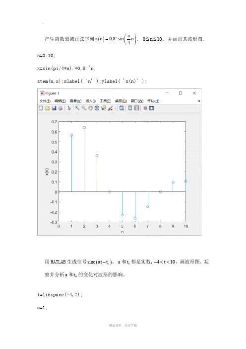
产生离散衰减正弦序列()π0.8sin 4n x n n ⎛⎫= ⎪⎝⎭, 010n ≤≤,并画出其波形图。
n=0:10;x=sin(pi/4*n).*0.8.^n;stem(n,x);xlabel( 'n' );ylabel( 'x(n)' );用MATLAB 生成信号()0sinc at t -, a 和0t 都是实数,410t -<<,画波形图。
观察并分析a 和0t 的变化对波形的影响。
t=linspace(-4,7); a=1;t0=2;y=sinc(a*t-t0); plot(t,y);t=linspace(-4,7); a=2;t0=2;y=sinc(a*t-t0); plot(t,y);t=linspace(-4,7); a=1;t0=2;y=sinc(a*t-t0); plot(t,y);三组对比可得a 越大最大值越小,t0越大图像对称轴越往右移某频率为f 的正弦波可表示为()()cos 2πa x t ft =,对其进行等间隔抽样,得到的离散样值序列可表示为()()a t nT x n x t ==,其中T 称为抽样间隔,代表相邻样值间的时间间隔,1s f T=表示抽样频率,即单位时间内抽取样值的个数。
抽样频率取40 Hz s f =,信号频率f 分别取5Hz, 10Hz, 20Hz 和30Hz 。
请在同一张图中同时画出连续信号()a x t t 和序列()x n nT 的波形图,并观察和对比分析样值序列的变化。
可能用到的函数为plot, stem, hold on 。
fs = 40;t = 0 : 1/fs : 1 ;% ƵÂÊ·Ö±ðΪ5Hz,10Hz,20Hz,30Hz f1=5;xa = cos(2*pi*f1*t) ; subplot(1, 2, 1) ;plot(t, xa) ;axis([0, max(t), min(xa), max(xa)]) ;xlabel('t(s)') ;ylabel('Xa(t)') ;line([0, max(t)],[0,0]) ; subplot(1, 2, 2) ;stem(t, xa, '.') ;line([0, max(t)], [0, 0]) ;axis([0, max(t), min(xa), max(xa)]) ;xlabel('n') ;ylabel('X(n)') ;频率越高,图像更加密集。
信号与系统实验答案

信号与系统实验答案% Q1_2clear, % Clear all variablesclose all, % Close all figure windowsdt = 0.01; % Specify the step of time variable t = 0:dt:2; % Specify the interval of time x = exp(-2*t); % Generate the signalplot(t,x) % Open a figure window and draw the plot of x(t)title('Sinusoidal signal x(t)')xlabel('Time t (sec)')axis([0,2,0,5])grid on>> % Q1_3clear, % Clear all variablesclose all, % Close all figure windowsdt = 0.01; % Specify the step of time variablet = 0:dt:2; % Specify the interval of timex = input('请输⼊任意信号x(t)'); % Generate the signalgrid onplot(t,x) % Open a figure window and draw the plot of x(t)title('Sinusoidal signal x(t)')xlabel('Time t (sec)')请输⼊任意信号x(t)exp(-2*t)Q1-4抄写函数⽂件delta如下:function y = delta(t)dt = 0.01;y = (u(t)-u(t-dt))/dt;抄写函数⽂件u如下:% Unit step functionfunction y = u(t)y = (t>=0); % y = 1 for t > 0, else y = 0%Q1_5clear, % Clear all variablesclose all, % Close all figure windowsn = -5:5; % Specify the interval of timex = [zeros(1,4), 0.1, 1.1, -1.2, 0, 1.3, zeros(1,2)]; % Generate the sequencestem (n,x,'.') % Open a figure window and draw the plot of x[n] grid on,axis([-2,5,-1.5,1.5])%Q1_6clear, % Clear all variablesclose all, % Close all figure windowsn = -5:5; % Specify the interval of timex =0.5.^abs(n); % Generate the sequencet=-2:0.01:5;y=cos(2*pi*t).*[u(t)-u(t-3)];subplot(2,1,1),stem (n,x,'.') ; % Open a figure window and draw the plot of x[n] grid on; title ('A discrete-time sequence x[n]')xlabel ('Time index n')subplot(2,1,2),plot (t,y) ;% Q1_7clear, % Clear all variablesclose all, % Close all figure windowsdt = 0.01; % Specify the step of time variablet = -5:dt:5; % Specify the interval of timex = exp(-0.5*t).*u(t); % Generate the signaly=exp(-0.75*t-1.5).*u(1.5*t+3);subplot(2,1,1),plot(t,x); % Open a figure window and draw the plot of x(t) grid on;title('Sinusoidal signal x(t)');xlabel('Time t (sec)');subplot(2,1,2),plot(t,y);grid on;title('Sinusoidal signal y(t)');xlabel('Time t (sec)');% Q1_8clear,close all,n = -20:20;x = u(n)-u(n-8); % Generate the original signal x(t)x1 = u(n+6)-u(n-2); % Shift x(t) to the left by 2 second to get x1(t)x2 = u(n-6)-u(n-14); % Shift x(t) to the right by 2 second to get x2(t)subplot(311),stem(n,x); % Plot x(t)grid on;title ('Original signal x(n)');subplot (312),stem (n,x1); % Plot x1(t)grid on;title ('Left shifted version of x(n)');subplot (313),stem (n,x2); % Plot x2(t)grid on;title ('Right shifted version of x(n)');xlabel ('Index n ');% Q1_9clear, close all;dt=0.01;t = -5:0.01:5;x = input('Type in the expression of the input signal x(t):');h = input('Type in the expression of the input signal h(t):');r=dt*conv(x,h);subplot(221), plot(t,x),title('x(t)');subplot(223), plot(t,h),title('h(t)');subplot(122),t = -10:0.01:10;plot(t,r); title('r(t)');% Q1_10clear;close all;n0 = -2; n1 = 10;n = n0:n1;x = 0.5.^n.*[u(n)-u(n-8)];h = u(n)-u(n-8);y = conv(x,h); % Compute the convolution of x(t) and h(t) subplot(311)stem(n,x), grid on, title('Signal x(n)'), axis([n0,n1,-0.2,1.2]) subplot(312)stem(n,h), grid on, title('Signal h(n)'), axis([n0,n1,-0.2,1.2]) subplot(313)n = 2*n0:2*n1; % Again specify the time range to be suitable to the % convolution of x and h.stem(n,y), grid on, title('The convolution of x(n) and h(n)'),xlabel('Index n')编写的程序Q1_11如下:clear, close all;n = -20:20;x=n.*[u(n)-u(n-4)];N = 8; y = 0;for k = -2:2;y =y+(n-k*N).*[u(n-k*N)-u(n-k*N-4)];endsubplot(211),stem(n,x); grid on, title('Signal x(n)'),subplot(212),stem(n,y); grid on, title('Signal y(n)'),% Q3_1b = input('请输⼊右边向量系数'); % The coefficient vector of the right side of the differential equationa = input('请输⼊左边向量系数'); % The coefficient vector of the left side of the differential equation[H,w] = freqs(b,a); % Compute the frequency response HHm = abs(H); % Compute the magnitude response Hmphai = angle(H); % Compute the phase response phaiHr = real(H); % Compute the real part of the frequency response Hi = imag(H); % Compute the imaginary part of the frequency responsesubplot(221)plot(w,Hm), grid on, title('Magnitude response'), xlabel('Frequency in rad/sec')subplot(223)plot(w,phai), grid on, title('Phase response'), xlabel('Frequency in rad/sec')subplot(222)plot(w,Hr), grid on, title('Real part of frequency response'),xlabel('Frequency in rad/sec')subplot(224)plot(w,Hi), grid on, title('Imaginary part of frequency response'), xlabel('Frequency in rad/sec')% Q3_2b = input('Type in the right coefficient vector of differential equation:'); % The coefficient vector of the right side of the differential equationa = input('Type in the left coefficient vector of differential equation:'); % The coefficient vector of the left side of the differential equationw=-10:0.01:10;H= freqs(b,a,w); % Compute the frequency response HHm = abs(H); % Compute the magnitude response Hmphai = angle(H); % Compute the phase response phaiHr = real(H); % Compute the real part of the frequency responseHi = imag(H); % Compute the imaginary part of the frequency responsesubplot(221);plot(w,Hm); grid on, title('Magnitude response'), xlabel('Frequency in rad/sec');subplot(223);plot(w,phai); grid on, title('Phase response'), xlabel('Frequency in rad/sec');subplot(222);plot(w,Hr); grid on, title('Real part of frequency response');xlabel('Frequency in rad/sec');subplot(224);plot(w,Hi); grid on, title('Imaginary part of frequency response');xlabel('Frequency in rad/sec');% Q3_3b1 = input('Type in the right coefficient vector of differential equation:'); % The coefficient vector of the right side of the differential equationa1= input('Type in the left coefficient vector of differential equation:'); % The coefficient vector of the left side of the differential equationb2 = input('Type in the right coefficient vector of differential equation:'); % The coefficient vector of the right side of the differential equationa2= input('Type in the left coefficient vector of differential equation:'); % The coefficient vector of the left side of the differential equationb3 = input('Type in the right coefficient vector of differential equation:'); % The coefficient vector of the right side of the differential equationa3= input('Type in the left coefficient vector of differential equation:'); % The coefficient vector of the left side of the differential equationw=-10:0.01:10;H1 = freqs(b1,a1,w); % Compute the frequency response Hphi1 = angle(H1);H2 = freqs(b2,a2,w); % Compute the frequency response Hphi2 = angle(H2);H3 = freqs(b3,a3,w); % Compute the frequency response Hphi3 = angle(H3);tao1= grpdelay(b1,a1,w);tao2= grpdelay(b2,a2,w);tao3= grpdelay(b3,a3,w);subplot(321);plot(w,phi1); grid on, title('Phase response of num1');subplot(323);plot(w,phi2); grid on, title('Phase response of num2');subplot(325);plot(w,phi3); grid on, title('Phase response of num3'), xlabel('Frequency in rad/sec'); subplot(322);plot(w,tao1); grid on, title('Group delay of num1');subplot(324);plot(w,tao2); grid on, title('Group delay of num2');subplot(326);plot(w,tao3); grid on, title('Group delay of num3'); xlabel('Frequency in rad/sec');。
信号与系统MATLAB仿真题目参考答案
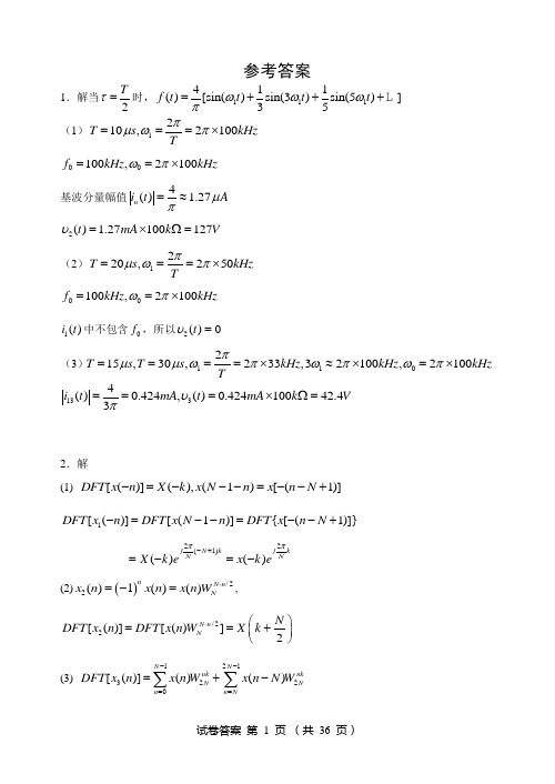
参考答案1.解当2T τ=时,111411()[sin()sin(3)sin(5)]35f t t t t ωωωπ=+++ (1)1210,2100T s kHz Tπμωπ===⨯ 00100,2100f kHz kHz ωπ==⨯基波分量幅值4() 1.27n i t A μπ=≈2() 1.27100127t mA k V υ=⨯Ω=(2)1220,250T s kHz Tπμωπ===⨯ 00100,2100f kHz kHz ωπ==⨯ 1()i t 中不包含0f ,所以2()0t υ=(3)110215,30,233,32100,2100T s T s kHz kHz kHz Tπμμωπωπωπ====⨯≈⨯=⨯ 1334()0.424,()0.42410042.43i t mA t mA k V υπ===⨯Ω= 2.解(1) [()](),(1)[(1)]DFT x n X k x N n x n N -=---=--+1[()][(1)]{[(1)]}DFT x n DFT x N n DFT x n N -=--=--+22(1)()()jN k jk NNX k ex k eππ-+=-=-(2)()/22()1()()nN n N x n x n x n W ⋅=-=,/22[()][()]2N n N N DFT x n DFT x n W X k ⋅⎛⎫==+ ⎪⎝⎭(3) 1213220[()]()()N N nknk NNn n NDFT x n x n Wx n N W--===+-∑∑1122200()()N N nk Nk nk NNNn n x n WWx n W--===+∑∑11/2/20()(1)N N nk knk nNn n x n WW--===+-∑∑2(/2)[1(1)]20k X k k k X k ⎧⎛⎫=+-=⎨⎪⎝⎭⎩为偶数为奇数(4) /214/2[()][()(/2)]N nk N n DFT x n x n x n N W-==++∑112(/2)/2/2/2()()N N nk n N kN N n n N x n Wx n W ---===+∑∑112/200()()(2)N N nknk N N n n x n Wx n W X k --⋅=====∑∑ (5) 2111/25220[()]()()()()2N N N nk nk nk s NNN n n n k DFT x n x n Wx n Wx n W X ---=======∑∑∑(6)DFT 216620[()]()N nk N n x n x n W -==∑216202N nk N n n n xW -=⎛⎫=⎪⎝⎭∑为偶21260()()2N N k k n n x W X k -===∑(7) 1/21277/2/20[()]()(2)N N nk nkN N n n DFT x n x n Wx n W --====∑∑,令2,2mn m n ==1127/200[()]()()m N N k mk N Nm m m m DFT x n x m Wx m W--====∑∑为偶为偶101[()(1)()]2N m mkNm x m x m W -==+-∑110011()(1)()22N N mk m mkN Nm m x m W x m W --===+-∑∑ 1[()()]22N x k x k =++3.解 210()c o s ()2f t f t t τω⎛⎫=- ⎪⎝⎭由频域卷积定理,有{}221()()2f t F ωπ==12f t τ⎧⎫⎛⎫-*⎨⎬ ⎪⎝⎭⎩⎭{}0cos()t ω由于 21()24E F Sa τωτω⎛⎫= ⎪⎝⎭由时移性质可得221224j E f t Sa eωτττωτ-⎧⎫⎛⎫⎛⎫-=⎨⎬ ⎪ ⎪⎝⎭⎝⎭⎩⎭ 而{}[]000cos()()()t ωπδωωδωω=++-所以0000()()22002222200222()()()444()()444j j j j j E F Sa e Sa e E e Sa e Sa e ωωτωωτωτωτωτωωτωωττωωωτωωττ+-----⎧⎫+-⎡⎤⎡⎤=+⎨⎬⎢⎥⎢⎥⎣⎦⎣⎦⎩⎭⎧⎫+-⎪⎪⎡⎤⎡⎤=+⎨⎬⎢⎥⎢⎥⎣⎦⎣⎦⎪⎪⎩⎭4.解 由题图可知,()f t 为偶函数,因而240240112()cos n T TT T b E a f t dt E t dt T T T ππ--=⎛⎫===⎪⎝⎭⎰⎰212410402()cos()4222cos cos ,222cos (1)cos (1)TT n T T a f t n dtT E t n t dt T T T T E n t n t dt T T T ωπππωππ-=⎛⎫⎛⎫=⋅= ⎪ ⎪⎝⎭⎝⎭⎧⎫⎡⎤⎡⎤=++-⎨⎬⎢⎥⎢⎥⎣⎦⎣⎦⎩⎭⎰⎰⎰211sin sin 2211,120,3,5,1,2cos ,2,4,6,(1)2n n E n n E n n E n n n πππππ⎡+-⎤⎛⎫⎛⎫ ⎪ ⎪⎢⎥⎝⎭⎝⎭⎢⎥=++-⎢⎥⎢⎥⎣⎦⎧=⎪⎪⎪==⋅⋅⋅⎨⎪⎪=⋅⋅⋅-⎪⎩从而11111111112222()cos()cos(2)cos(4)cos(6)(8)231535634442cos()cos(2)cos(4)cos(6),231535EE E E E Ef t t t t t t E E t t t t T ωωωωωππππππωωωωωππππ=++-+-+⋅⋅⋅⎡⎤=++-++⋅⋅⋅=⎢⎥⎣⎦若E=10V ,f=10kHz ,则幅度谱如下图所示。
长江大学信号与系统matlab实验答案
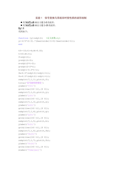
实验1 信号变换与系统非时变性质的波形绘制●用MA TLAB画出习题1-8的波形。
●用MA TLAB画出习题1-10的波形。
Eg 1.8代码如下:function [y]=zdyt(t) %定义函数zdyty=-2/3*(t-3).*(heaviside(-t+3)-heaviside(-t));endt0=-10;t1=4;dt=0.02;t=t0:dt:t1;f=zdyt(t);y=zdyt(t+3);x=zdyt(2*t-2);g=zdyt(2-2*t);h=zdyt(-0.5*t-1);fe=0.5*(zdyt(t)+zdyt(-t));fo=0.5*(zdyt(t)-zdyt(-t));subplot(7,1,1),plot(t,f);title('信号波形的变化')ylabel('f(t)')grid;line([t0 t1],[0 0]);subplot(7,1,2),plot(t,y);ylabel('y(t)')grid;line([t0 t1],[0 0]);subplot(7,1,3),plot(t,x);ylabel('x(t)')grid;line([t0 t1],[0 0]);subplot(7,1,4),plot(t,g);ylabel('g(t)')grid;line([t0 t1],[0 0]);subplot(7,1,5),plot(t,h);ylabel('h(t)')grid;line([t0 t1],[0 0]);subplot(7,1,6),plot(t,fe);ylabel('fe(t)')grid;line([t0 t1],[0 0]);subplot(7,1,7),plot(t,fo);ylabel('fo(t)')grid;line([t0 t1],[0 0]);xlabel('Time(sec)')结果:Eg1.10代码如下:function [u]=f(t) %定义函数f(t) u= heaviside(t)-heaviside(t-2); endfunction [u] =y(t) %定义函数y(t)u=2*(t.*heaviside(t)-2*(t-1).*heaviside(t-1)+(t-2).*heaviside(t-2)); endt0=-2;t1=5;dt=0.01; t=t0:dt:t1; f1=f(t); y1=y(t); f2=f(t)-f(t-2); y2=y(t)-y(t-2); f3=f(t)-f(t+1); y3=y(t)-y(t+1);subplot(3,2,1),plot(t,f1); title('激励——响应波形图') ylabel('f1(t)')grid;line([t0 t1],[0 0]);-10-8-6-4-2024012信号波形的变化f (t)-10-8-6-4-2024012y (t)-10-8-6-4-2024012x (t)-10-8-6-4-2024012g (t)-10-8-6-4-2024012h (t)-10-8-6-4-202400.51f e (t)-10-8-6-4-2024-101f o (t)Time(sec)subplot(3,2,2),plot(t,y1); ylabel('y1(t)')grid;line([t0 t1],[0 0]); subplot(3,2,3),plot(t,f2); ylabel('f2(t)')grid;line([t0 t1],[0 0]); subplot(3,2,4),plot(t,y2); ylabel('y2(t)')grid;line([t0 t1],[0 0]); subplot(3,2,5),plot(t,f3); ylabel('f3(t)')grid;line([t0 t1],[0 0]); subplot(3,2,6),plot(t,y3); ylabel('y3(t)')grid;line([t0 t1],[0 0]); xlabel('Time(sec)')结果:实验2 微分方程的符号计算和波形绘制上机内容用MA TLAB 计算习题2-1,并画出系统响应的波形。
基于MATLAB的信号与系统实验教程

基于MATLAB的信号与系统实验教程第一部分 MATLAB基础第1章 MATLAB环境1.1 MATLAB界面图1.1 MATLAB主界面图1.2 Workspace图1.3 MATLAB.m文件编辑窗口界面1.2 文件类型图1.4 设置路径图1.5 例1-1运行结果1.3 系统和程序控制指令1.4 练习第2章 数据类型与数学运算2.1 数值、变量和表达式2.1.1 数值的记述2.1.2 变量命名规则2.1.3 运算符和表达式2.2 数组、矩阵及其运算2.2.1 复数和复数矩阵2.2.2 数组和矩阵的运算2.2.3 特殊矩阵(Specialized matrices)2.3 关系和逻辑运算2.4 练习第3章 数值计算与符号计算3.1 线性代数与矩阵分析3.1.1 线性代数3.1.2 特征值分解3.1.3 奇异值分解3.1.4 矩阵函数3.2 线性方程组求解3.2.1 确定性线性方程组求解3.2.2 线性最小二乘问题的方程求解3.3 数据分析函数图3.1 例3-4运行结果3.4 符号计算图3.2 数值型与符号型数据转换关系3.5 练习第4章 绘图4.1 基本绘图指令4.1.1 plot的基本调用格式图4.1 例4-1运行结果4.1.2 stem: 离散数据绘制(火柴杆图)图4.2 例4-2运行结果4.1.3 polar: 极坐标图图4.3 例4-3运行结果4.2 各种图形标记、控制指令图4.4 例4-4运行结果4.2.1 图的创建与控制4.2.2 轴的产生与控制4.2.3 分格线(grid)、坐标框(box)、图保持(hold)4.2.4 图形标志4.3 其他常用绘图指令4.3.1 其他类型图的绘制图4.5 例4-5运行结果图4.6 例4-6运行结果简易绘图指令图4.7 例4-7运行结果4.4 练习第5章 SIMULINK5.1 SIMULINK的基本使用方法图5.1 Simulink Library Browser窗口图5.2 Pulse Generator模块的参数设置5.2 SIMULINK模型概念及基本模块介绍图5.4 SIMULINK模型的一般结构5.2.1 常用的sources——信号源模块5.2.2 常用的sinks——信号显示与输出模块图5.5 示波器纵坐标设置对话框图5.6 示波器属性对话框5.2.3 math operations——数学运算单元模块5.2.4 continuous——连续系统模块5.2.5 discrete——离散系统模块5.3 SIMULINK模型的仿真5.3.1 仿真参数设置图5.7 仿真设置对话框5.3.2 建立子系统图5.8 例5-2的SIMULINK模型图5.9 例5-2的子系统模型图5.10 例5-2仿真输出波形5.4 练习第6章 M函数和工具箱6.1 M函数6.2 工具箱图6.1 演示程序中的工具箱(Toolbox)使用帮助6.3 练习第7章 MATLAB实用技术遴选7.1 图形用户界面设计7.1.1 设计原则与设计步骤7.1.2 界面与控件介绍图7.1 标准菜单样式7.1.3 GUI实例分析。
信号与系统matlab课后作业-北京交通大学
信号与系统MATLAB平时作业学院:电子信息工程学院班级::学号:教师:钱满义MATLAB 习题M3-1 一个连续时间LTI系统满足的微分方程为y ’’(t)+3y ’(t)+2y(t)=2x ’(t)+x(t)(1)已知x(t)=e -3t u(t),试求该系统的零状态响应y zs (t); (2)用lism 求出该系统的零状态响应的数值解。
利用(1)所求得的结果,比较不同的抽样间隔对数值解精度的影响。
解:(1) 由于''()3'()2()2'()(),0h t h t h t t t t δδ++=+≥则2()()()t t h t Ae Be u t --=+ 将()h t 带入原方程式化简得(2)()()'()2'()()A B t A B t t t δδδδ+++=+所以1,3A B =-=2()(3)()t t h t e e u t --=-+又因为3t ()()x t e u t -= 则该系统的零状态响应3t 23t 2t ()()()()(3)()0.5(6+5)()zs t t t y t x t h t e u t e e u t e e e u t ----=*=*-+=-- (2)程序代码 1、ts=0;te=5;dt=0.1;sys=tf([2 1],[1 3 2]);t=ts:dt:te;x=exp(-3*t).*(t>=0);y=lsim(sys,x,t)2、ts=0;te=5;dt=1;sys=tf([2 1],[1 3 2]);t=ts:dt:te;x=exp(-3*t).*(t>=0);y1=-0.5*exp(-3*t).*(exp(2*t)-6*exp(t)+5).*[t>=0];y2=lsim(sys,x,t)plot(t,y1,'r-',t,y2,'b--')xlabel('Time(sec)')legend('实际值','数值解')用lism求出的该系统的零状态响应的数值解在不同的抽样间隔时与(1)中求出的实际值进行比较将两种结果画在同一幅图中有图表 1 抽样间隔为1图表 2 抽样间隔为0.1图表 3 抽样间隔为0.01当抽样间隔dt减小时,数值解的精度越来越高,从图像上也可以看出数值解曲线越来越逼近实际值曲线,直至几乎重合。
信号与系统第七章课后答案
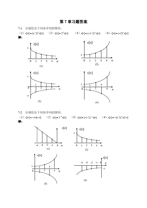
7-1 分别绘出下列各序列的图形。 (2)x[n] 2n u[n] (3)x[n] (1/ 2)n u[n] (4)x[n] (2) n u[ n] (1)x[n] (1/ 2)n u[n] 解:
x[ n ]
1
x[n]
1
0 1 2 (1) 3 4
n
0
1
2 3 (2)
x[n]
1
x[n]
-4
-3
-2 (1)
-1
0
n
0
1
2 (2)
3
4
n
x[n]
-4 1 0 1 2 3 4 -3 -2 -1 0
x[n] n
-1
n
(4)
(3)
7-3
分别绘出下列各序列的图形。 (2) x[n] cos
n 10 5
n (1) x[n] sin 5
1 z2 X (z) ( 1 1 2 z 1 )( 1 2 z 1 ) ( z 1 2 )( z 2 ) X (z) z 1 4 z ( z 1 2 )( z 2 ) 3( z 1 2 ) 3( z 2 )
X (z)
z 4z 3( z 1 2 ) 3 ( z 2 )
N
)
由于 x[n] 、 h[n] 均为因果序列,因此 y[n] 亦为因果序列,根据移位性质可求得
y [ n ] Z 1 [Y ( z )]
1 1 (1 a n 1 ) u [ n ] (1 a n 1 N ) u [ n N ] 1 a 1 a
7-24 计算下列序列的傅里叶变换。
(2)