图像预处理代码
transforms.resize参数
transforms.resize参数1.简介在图像处理中,尺寸调整(r es iz e)是一项常见的操作。
在深度学习中,数据的预处理过程中,r es iz e操作被广泛应用于图像的预处理中。
P y To rch中提供了t r an sf or ms模块,其中包含了多种尺寸调整的方法,本文将详细介绍t ran s fo rm s中re si ze方法的参数。
2. tr ansforms.resiz e方法在t ra ns fo rm s模块中,re si ze方法用于调整图像的大小。
其基本语法结构如下:t r an sf or ms.R es ize(si ze,i nt er po lat i on=I nt er po la tio n Mo de.B I LI NE AR)参数说明:-s iz e:调整后的图像大小,可以是一个整数或一个元组。
若为整数,则表示图像的长宽按比例缩放;若为元组,则表示图像的长宽分别缩放到指定大小。
-i nt er po la ti on:插值方式,用于定义缩放时的插值方法。
可选值有`I nt er po la ti on Mod e.N EA RE ST`、`I nt e rp ol at io nM od e.B I LI NE AR`和`In te rp ol at io nM o de.B IC UB IC`。
3.参数详解3.1s i z e参数s i ze参数用于定义调整后的图像大小。
它可以是一个整数,表示调整后的图像按比例缩放;也可以是一个元组,表示图像的长宽分别缩放到指定大小。
3.1.1整数当s iz e参数为一个整数时,图像的长宽按相同的比例进行缩放。
例如,调整图像为100x100像素大小,可以使用如下方式:t r an sf or ms.R es ize(100)3.1.2元组当s iz e参数为一个元组时,图像的长宽可以分别指定。
例如,调整图像的长为100像素,宽为200像素,可以使用如下方式:t r an sf or ms.R es ize((100,200))3.2i n t e r p o l a t i o n参数i n te rp ol at io n参数用于定义缩放时的插值方法,即在图像缩放时如何计算非整数像素的值。
C语言实现图像识别
C语言实现图像识别图像识别是计算机视觉领域的重要研究方向之一,它通过算法和模型实现计算机对图像内容的理解和分类。
C语言是一种通用的高级编程语言,具有高效性和强大的计算能力,因此在图像识别领域中也有广泛的应用。
本文将介绍C语言在图像识别方面的应用和实现。
一、图像预处理在进行图像识别之前,首先需要对图像进行预处理。
图像预处理的目的是去除图像中的噪声、调整图像的对比度和亮度等,从而更好地提取图像特征。
在C语言中,我们可以使用各种图像处理库,如OpenCV来实现图像预处理。
下面是一个简单的C语言代码示例,演示了如何使用OpenCV对图像进行预处理:```C#include <opencv2/opencv.hpp>using namespace cv;int main(){// 读取图像Mat image = imread("image.jpg", IMREAD_COLOR);// 转为灰度图像cvtColor(image, image, COLOR_BGR2GRAY);// 高斯模糊GaussianBlur(image, image, Size(5, 5), 0);// 边缘检测Canny(image, image, 50, 150);// 显示图像imshow("Processed Image", image);waitKey(0);return 0;}```二、特征提取在进行图像识别之前,还需要提取图像的特征。
特征提取是将图像转换为计算机可理解的数值形式,以便进行进一步的处理和分类。
C 语言提供了各种特征提取的方法和算法的实现,下面是一个简单的C 语言代码示例,演示了如何使用C语言进行图像特征提取:```C#include <stdio.h>int main(){// 读取图像特征数据float features[100];FILE *file = fopen("features.txt", "r");for (int i = 0; i < 100; i++) {fscanf(file, "%f", &features[i]);}fclose(file);// 进行图像分类或其他处理// ...return 0;}```三、模型训练与识别在进行图像识别之前,需要训练一个模型来对图像进行分类。
数字图像处理代码大全

1.图像反转MATLAB程序实现如下:I=imread('xian.bmp');J=double(I);J=-J+(256-1); %图像反转线性变换H=uint8(J);subplot(1,2,1),imshow(I);subplot(1,2,2),imshow(H);2.灰度线性变换MATLAB程序实现如下:I=imread('xian.bmp');subplot(2,2,1),imshow(I);title('原始图像');axis([50,250,50,200]);axis on; %显示坐标系I1=rgb2gray(I);subplot(2,2,2),imshow(I1);title('灰度图像');axis([50,250,50,200]);axis on; %显示坐标系J=imadjust(I1,[0.1 0.5],[]); %局部拉伸,把[0.1 0.5]内的灰度拉伸为[0 1]subplot(2,2,3),imshow(J);title('线性变换图像[0.1 0.5]');axis([50,250,50,200]);grid on; %显示网格线axis on; %显示坐标系K=imadjust(I1,[0.3 0.7],[]); %局部拉伸,把[0.3 0.7]内的灰度拉伸为[0 1]subplot(2,2,4),imshow(K);title('线性变换图像[0.3 0.7]');axis([50,250,50,200]);grid on; %显示网格线axis on; %显示坐标系3.非线性变换MATLAB程序实现如下:I=imread('xian.bmp');I1=rgb2gray(I);subplot(1,2,1),imshow(I1);title('灰度图像');axis([50,250,50,200]);grid on; %显示网格线axis on; %显示坐标系J=double(I1);J=40*(log(J+1));H=uint8(J);subplot(1,2,2),imshow(H);title('对数变换图像');axis([50,250,50,200]);grid on; %显示网格线axis on; %显示坐标系4.直方图均衡化MATLAB程序实现如下:I=imread('xian.bmp');I=rgb2gray(I);figure;subplot(2,2,1);imshow(I);subplot(2,2,2);imhist(I);I1=histeq(I);figure;subplot(2,2,1);imshow(I1);subplot(2,2,2);imhist(I1);5.线性平滑滤波器用MATLAB实现领域平均法抑制噪声程序:I=imread('xian.bmp');subplot(231)imshow(I)title('原始图像')I=rgb2gray(I);I1=imnoise(I,'salt & pepper',0.02);subplot(232)imshow(I1)title('添加椒盐噪声的图像')k1=filter2(fspecial('average',3),I1)/255; %进行3*3模板平滑滤波k2=filter2(fspecial('average',5),I1)/255; %进行5*5模板平滑滤波k3=filter2(fspecial('average',7),I1)/255; %进行7*7模板平滑滤波k4=filter2(fspecial('average',9),I1)/255; %进行9*9模板平滑滤波subplot(233),imshow(k1);title('3*3模板平滑滤波');subplot(234),imshow(k2);title('5*5模板平滑滤波');subplot(235),imshow(k3);title('7*7模板平滑滤波');subplot(236),imshow(k4);title('9*9模板平滑滤波'); 6.中值滤波器用MATLAB实现中值滤波程序如下:I=imread('xian.bmp');I=rgb2gray(I);J=imnoise(I,'salt&pepper',0.02);subplot(231),imshow(I);title('原图像');subplot(232),imshow(J);title('添加椒盐噪声图像');k1=medfilt2(J); %进行3*3模板中值滤波k2=medfilt2(J,[5,5]); %进行5*5模板中值滤波k3=medfilt2(J,[7,7]); %进行7*7模板中值滤波k4=medfilt2(J,[9,9]); %进行9*9模板中值滤波subplot(233),imshow(k1);title('3*3模板中值滤波'); subplot(234),imshow(k2);title('5*5模板中值滤波'); subplot(235),imshow(k3);title('7*7模板中值滤波'); subplot(236),imshow(k4);title('9*9模板中值滤波'); 7.用Sobel算子和拉普拉斯对图像锐化:I=imread('xian.bmp');subplot(2,2,1),imshow(I);title('原始图像');axis([50,250,50,200]);grid on; %显示网格线axis on; %显示坐标系I1=im2bw(I);subplot(2,2,2),imshow(I1);title('二值图像');axis([50,250,50,200]);grid on; %显示网格线axis on; %显示坐标系H=fspecial('sobel'); %选择sobel算子J=filter2(H,I1); %卷积运算subplot(2,2,3),imshow(J);title('sobel算子锐化图像');axis([50,250,50,200]);grid on; %显示网格线axis on; %显示坐标系h=[0 1 0,1 -4 1,0 1 0]; %拉普拉斯算子J1=conv2(I1,h,'same'); %卷积运算subplot(2,2,4),imshow(J1);title('拉普拉斯算子锐化图像');axis([50,250,50,200]);grid on; %显示网格线axis on; %显示坐标系8.梯度算子检测边缘用MATLAB实现如下:I=imread('xian.bmp');subplot(2,3,1);imshow(I);title('原始图像');axis([50,250,50,200]);grid on; %显示网格线axis on; %显示坐标系I1=im2bw(I);subplot(2,3,2);imshow(I1);title('二值图像');axis([50,250,50,200]);grid on; %显示网格线axis on; %显示坐标系I2=edge(I1,'roberts');figure;subplot(2,3,3);imshow(I2);title('roberts算子分割结果');axis([50,250,50,200]);grid on; %显示网格线axis on; %显示坐标系I3=edge(I1,'sobel');subplot(2,3,4);imshow(I3);title('sobel算子分割结果');axis([50,250,50,200]);grid on; %显示网格线axis on; %显示坐标系I4=edge(I1,'Prewitt');subplot(2,3,5);imshow(I4);title('Prewitt算子分割结果');axis([50,250,50,200]);grid on; %显示网格线axis on; %显示坐标系9.LOG算子检测边缘用MATLAB程序实现如下:I=imread('xian.bmp');subplot(2,2,1);imshow(I);title('原始图像');I1=rgb2gray(I);subplot(2,2,2);imshow(I1);title('灰度图像');I2=edge(I1,'log');subplot(2,2,3);imshow(I2);title('log算子分割结果'); 10.Canny算子检测边缘用MATLAB程序实现如下:I=imread('xian.bmp'); subplot(2,2,1);imshow(I);title('原始图像')I1=rgb2gray(I);subplot(2,2,2);imshow(I1);title('灰度图像');I2=edge(I1,'canny'); subplot(2,2,3);imshow(I2);title('canny算子分割结果');11.边界跟踪(bwtraceboundary函数)clcclear allI=imread('xian.bmp');figureimshow(I);title('原始图像');I1=rgb2gray(I); %将彩色图像转化灰度图像threshold=graythresh(I1); %计算将灰度图像转化为二值图像所需的门限BW=im2bw(I1, threshold); %将灰度图像转化为二值图像figureimshow(BW);title('二值图像');dim=size(BW);col=round(dim(2)/2)-90; %计算起始点列坐标row=find(BW(:,col),1); %计算起始点行坐标connectivity=8;num_points=180;contour=bwtraceboundary(BW,[row,col],'N',connectivity,num_p oints);%提取边界figureimshow(I1);hold on;plot(contour(:,2),contour(:,1), 'g','LineWidth' ,2); title('边界跟踪图像');12.Hough变换I= imread('xian.bmp');rotI=rgb2gray(I);subplot(2,2,1);imshow(rotI);title('灰度图像');axis([50,250,50,200]);grid on;axis on;BW=edge(rotI,'prewitt');subplot(2,2,2);imshow(BW);title('prewitt算子边缘检测后图像');axis([50,250,50,200]);grid on;axis on;[H,T,R]=hough(BW);subplot(2,2,3);imshow(H,[],'XData',T,'YData',R,'InitialMagnification','fit'); title('霍夫变换图');xlabel('\theta'),ylabel('\rho');axis on , axis normal, hold on;P=houghpeaks(H,5,'threshold',ceil(0.3*max(H(:))));x=T(P(:,2));y=R(P(:,1));plot(x,y,'s','color','white');lines=houghlines(BW,T,R,P,'FillGap',5,'MinLength',7); subplot(2,2,4);,imshow(rotI);title('霍夫变换图像检测');axis([50,250,50,200]);grid on;axis on;hold on;max_len=0;for k=1:length(lines)xy=[lines(k).point1;lines(k).point2];plot(xy(:,1),xy(:,2),'LineWidth',2,'Color','green');plot(xy(1,1),xy(1,2),'x','LineWidth',2,'Color','yellow');plot(xy(2,1),xy(2,2),'x','LineWidth',2,'Color','red');len=norm(lines(k).point1-lines(k).point2);if(len>max_len)max_len=len;xy_long=xy;endendplot(xy_long(:,1),xy_long(:,2),'LineWidth',2,'Color','cyan'); 13.直方图阈值法用MATLAB实现直方图阈值法:I=imread('xian.bmp');I1=rgb2gray(I);figure;subplot(2,2,1);imshow(I1);title('灰度图像')axis([50,250,50,200]);grid on; %显示网格线axis on; %显示坐标系[m,n]=size(I1); %测量图像尺寸参数GP=zeros(1,256); %预创建存放灰度出现概率的向量for k=0:255GP(k+1)=length(find(I1==k))/(m*n); %计算每级灰度出现的概率,将其存入GP中相应位置endsubplot(2,2,2),bar(0:255,GP,'g') %绘制直方图title('灰度直方图')xlabel('灰度值')ylabel('出现概率')I2=im2bw(I,150/255);subplot(2,2,3),imshow(I2);title('阈值150的分割图像')axis([50,250,50,200]);grid on; %显示网格线axis on; %显示坐标系I3=im2bw(I,200/255); %subplot(2,2,4),imshow(I3);title('阈值200的分割图像')axis([50,250,50,200]);grid on; %显示网格线axis on; %显示坐标系14. 自动阈值法:Otsu法用MATLAB实现Otsu算法:clcclear allI=imread('xian.bmp');subplot(1,2,1),imshow(I);title('原始图像')axis([50,250,50,200]);grid on; %显示网格线axis on; %显示坐标系level=graythresh(I); %确定灰度阈值BW=im2bw(I,level);subplot(1,2,2),imshow(BW);title('Otsu法阈值分割图像')axis([50,250,50,200]);grid on; %显示网格线axis on; %显示坐标系15.膨胀操作I=imread('xian.bmp'); %载入图像I1=rgb2gray(I);subplot(1,2,1);imshow(I1);title('灰度图像')axis([50,250,50,200]);grid on; %显示网格线axis on; %显示坐标系se=strel('disk',1); %生成圆形结构元素I2=imdilate(I1,se); %用生成的结构元素对图像进行膨胀subplot(1,2,2);imshow(I2);title('膨胀后图像');axis([50,250,50,200]);grid on; %显示网格线axis on; %显示坐标系16.腐蚀操作MATLAB实现腐蚀操作I=imread('xian.bmp'); %载入图像I1=rgb2gray(I);subplot(1,2,1);imshow(I1);title('灰度图像')axis([50,250,50,200]);grid on; %显示网格线axis on; %显示坐标系se=strel('disk',1); %生成圆形结构元素I2=imerode(I1,se); %用生成的结构元素对图像进行腐蚀subplot(1,2,2);imshow(I2);title('腐蚀后图像');axis([50,250,50,200]);grid on; %显示网格线axis on; %显示坐标系17.开启和闭合操作用MATLAB实现开启和闭合操作I=imread('xian.bmp'); %载入图像subplot(2,2,1),imshow(I);title('原始图像');axis([50,250,50,200]);axis on; %显示坐标系I1=rgb2gray(I);subplot(2,2,2),imshow(I1);title('灰度图像');axis([50,250,50,200]);axis on; %显示坐标系se=strel('disk',1); %采用半径为1的圆作为结构元素I3=imclose(I1,se); %闭合操作subplot(2,2,3),imshow(I2);title('开启运算后图像');axis([50,250,50,200]);axis on; %显示坐标系subplot(2,2,4),imshow(I3);title('闭合运算后图像');axis([50,250,50,200]);axis on; %显示坐标系18.开启和闭合组合操作I=imread('xian.bmp'); %载入图像subplot(3,2,1),imshow(I);title('原始图像');axis([50,250,50,200]);axis on; %显示坐标系I1=rgb2gray(I);subplot(3,2,2),imshow(I1);title('灰度图像');axis([50,250,50,200]);axis on; %显示坐标系se=strel('disk',1);I3=imclose(I1,se); %闭合操作subplot(3,2,3),imshow(I2);title('开启运算后图像');axis([50,250,50,200]);axis on; %显示坐标系subplot(3,2,4),imshow(I3);title('闭合运算后图像');axis([50,250,50,200]);axis on; %显示坐标系se=strel('disk',1);I4=imopen(I1,se);I5=imclose(I4,se);subplot(3,2,5),imshow(I5); %开—闭运算图像title('开—闭运算图像');axis([50,250,50,200]);axis on; %显示坐标系I6=imclose(I1,se);I7=imopen(I6,se);subplot(3,2,6),imshow(I7); %闭—开运算图像title('闭—开运算图像');axis([50,250,50,200]);axis on; %显示坐标系19.形态学边界提取利用MATLAB实现如下:I=imread('xian.bmp'); %载入图像subplot(1,3,1),imshow(I);title('原始图像');axis([50,250,50,200]);grid on; %显示网格线axis on; %显示坐标系I1=im2bw(I);subplot(1,3,2),imshow(I1);title('二值化图像');axis([50,250,50,200]);grid on; %显示网格线axis on; %显示坐标系I2=bwperim(I1); %获取区域的周长subplot(1,3,3),imshow(I2);title('边界周长的二值图像');axis([50,250,50,200]);grid on;axis on;20.形态学骨架提取利用MATLAB实现如下:I=imread('xian.bmp'); subplot(2,2,1),imshow(I); title('原始图像');axis([50,250,50,200]); axis on;I1=im2bw(I);subplot(2,2,2),imshow(I1); title('二值图像');axis([50,250,50,200]); axis on;I2=bwmorph(I1,'skel',1); subplot(2,2,3),imshow(I2); title('1次骨架提取');axis([50,250,50,200]); axis on;I3=bwmorph(I1,'skel',2); subplot(2,2,4),imshow(I3); title('2次骨架提取');axis([50,250,50,200]); axis on;21.直接提取四个顶点坐标I = imread('xian.bmp');I = I(:,:,1);BW=im2bw(I);figureimshow(~BW)[x,y]=getpts。
msl数据集的预处理代码_示例及概述说明
msl数据集的预处理代码示例及概述说明1. 引言1.1 概述:在当今科技发展的时代,数据分析和机器学习等领域正变得越来越重要。
而在这些领域中,数据集的质量和准确性对于研究和应用的成功起着至关重要的作用。
MSL(Machine Symbolic Learning)数据集是一个被广泛使用和研究的公开数据集,其中包含了大量有关机器学习算法性能评估的信息。
本文旨在介绍MSL数据集的预处理代码示例,并提供详细说明。
通过本文,读者将能够了解如何进行MSL数据集的预处理,以及预处理过程中所需考虑的一些关键步骤和技巧。
本文还将提供一些用于数据清洗、特征工程以及标签处理等方面的代码示例,并以简洁明了的方式阐述其背后的原理。
1.2 文章结构:本文按照以下结构组织:首先,我们将在第2节介绍MSL数据集,并对其内容进行概述。
接下来,在第3节中,我们将详细介绍MSL数据集预处理过程中的第一部分步骤,并给出相关代码示例。
随后,在第4节中,我们将进一步探讨预处理过程中的第二部分步骤,同样提供相应的代码示例。
最后,在第5节中,我们将进行总结,并探讨进一步研究方向。
1.3 目的:本文的目的是为读者提供一个全面且易于理解的MSL数据集预处理指南,为从事机器学习和数据分析领域的研究人员和开发者们提供有价值的参考资料。
通过了解MSL数据集预处理过程中的关键步骤和示例代码,读者将能够更好地应用这些技术和工具来处理其他类似领域中的问题。
无论是初学者还是经验丰富的专业人士,本文都将有助于拓宽他们在数据预处理方面的知识和技能,进而在实际应用中取得更好的结果。
2. MSL数据集预处理代码示例2.1 数据集介绍在本节中,我们将介绍MSL(Mars Science Laboratory)数据集,该数据集是由NASA的Curiosity火星车通过其Mastcam仪器拍摄的一系列图像组成的。
这些图像被用于研究和探索火星表面的地质特征和环境。
2.2 预处理步骤一在本节中,我们将展示MSL数据集的预处理代码示例的第一步。
halcon教程
halcon教程Halcon是一种广泛应用于机器视觉领域的软件库,它提供了丰富的图像处理和分析功能。
本教程将介绍Halcon的基本使用方法,涵盖图像读取、预处理、特征提取、目标检测等常用操作。
1. 图像读取使用Halcon的read_image函数可以从文件中读取图像数据。
可以通过指定文件路径来读取图像,例如:read_image(Image, 'image.jpg')2. 图像预处理在图像处理之前,通常需要对图像进行一些预处理操作,以改善后续处理的效果。
Halcon提供了丰富的预处理函数,如灰度化、平滑、滤波等。
例如,可以使用以下代码对图像进行灰度化处理:gray_image(Image, GrayImage)3. 特征提取Halcon提供了多种特征提取函数,可以从图像中获取有用的信息。
常用的特征包括边缘、角点、斑点等。
例如,可以使用find_edges函数在图像中提取边缘信息:find_edges(GrayImage, Edges, 10, 40)4. 目标检测目标检测是机器视觉中的一个重要任务,Halcon提供了多种目标检测函数和算法。
例如,可以使用find_shape_models函数对图像中的形状进行检测:find_shape_models(GrayImage, Model, AngleStart, AngleExtent, MinScore, NumMatches, SubPixel, Greediness, Result)以上是一些Halcon的基本用法,通过学习这些基础知识,您可以在机器视觉应用中更好地运用Halcon库进行图像处理和分析。
希望这些信息对您有所帮助!。
(完整版)数字图像处理代码大全

1.图像反转MATLAB程序实现如下:I=imread('xian.bmp');J=double(I);J=-J+(256-1); %图像反转线性变换H=uint8(J);subplot(1,2,1),imshow(I);subplot(1,2,2),imshow(H);2.灰度线性变换MATLAB程序实现如下:I=imread('xian.bmp');subplot(2,2,1),imshow(I);title('原始图像');axis([50,250,50,200]);axis on; %显示坐标系I1=rgb2gray(I);subplot(2,2,2),imshow(I1);title('灰度图像');axis([50,250,50,200]);axis on; %显示坐标系J=imadjust(I1,[0.1 0.5],[]); %局部拉伸,把[0.1 0.5]内的灰度拉伸为[0 1]subplot(2,2,3),imshow(J);title('线性变换图像[0.1 0.5]');axis([50,250,50,200]);grid on; %显示网格线axis on; %显示坐标系K=imadjust(I1,[0.3 0.7],[]); %局部拉伸,把[0.3 0.7]内的灰度拉伸为[0 1]subplot(2,2,4),imshow(K);title('线性变换图像[0.3 0.7]');axis([50,250,50,200]);grid on; %显示网格线axis on; %显示坐标系3.非线性变换MATLAB程序实现如下:I=imread('xian.bmp');I1=rgb2gray(I);subplot(1,2,1),imshow(I1);title('灰度图像');axis([50,250,50,200]);grid on; %显示网格线axis on; %显示坐标系J=double(I1);J=40*(log(J+1));H=uint8(J);subplot(1,2,2),imshow(H);title('对数变换图像');axis([50,250,50,200]);grid on; %显示网格线axis on; %显示坐标系4.直方图均衡化MATLAB程序实现如下:I=imread('xian.bmp');I=rgb2gray(I);figure;subplot(2,2,1);imshow(I);subplot(2,2,2);imhist(I);I1=histeq(I);figure;subplot(2,2,1);imshow(I1);subplot(2,2,2);imhist(I1);5.线性平滑滤波器用MATLAB实现领域平均法抑制噪声程序:I=imread('xian.bmp');subplot(231)imshow(I)title('原始图像')I=rgb2gray(I);I1=imnoise(I,'salt & pepper',0.02);subplot(232)imshow(I1)title('添加椒盐噪声的图像')k1=filter2(fspecial('average',3),I1)/255; %进行3*3模板平滑滤波k2=filter2(fspecial('average',5),I1)/255; %进行5*5模板平滑滤波k3=filter2(fspecial('average',7),I1)/255; %进行7*7模板平滑滤波k4=filter2(fspecial('average',9),I1)/255; %进行9*9模板平滑滤波subplot(233),imshow(k1);title('3*3模板平滑滤波');subplot(234),imshow(k2);title('5*5模板平滑滤波');subplot(235),imshow(k3);title('7*7模板平滑滤波');subplot(236),imshow(k4);title('9*9模板平滑滤波'); 6.中值滤波器用MATLAB实现中值滤波程序如下:I=imread('xian.bmp');I=rgb2gray(I);J=imnoise(I,'salt&pepper',0.02);subplot(231),imshow(I);title('原图像');subplot(232),imshow(J);title('添加椒盐噪声图像');k1=medfilt2(J); %进行3*3模板中值滤波k2=medfilt2(J,[5,5]); %进行5*5模板中值滤波k3=medfilt2(J,[7,7]); %进行7*7模板中值滤波k4=medfilt2(J,[9,9]); %进行9*9模板中值滤波subplot(233),imshow(k1);title('3*3模板中值滤波'); subplot(234),imshow(k2);title('5*5模板中值滤波'); subplot(235),imshow(k3);title('7*7模板中值滤波'); subplot(236),imshow(k4);title('9*9模板中值滤波'); 7.用Sobel算子和拉普拉斯对图像锐化:I=imread('xian.bmp');subplot(2,2,1),imshow(I);title('原始图像');axis([50,250,50,200]);grid on; %显示网格线axis on; %显示坐标系I1=im2bw(I);subplot(2,2,2),imshow(I1);title('二值图像');axis([50,250,50,200]);grid on; %显示网格线axis on; %显示坐标系H=fspecial('sobel'); %选择sobel算子J=filter2(H,I1); %卷积运算subplot(2,2,3),imshow(J);title('sobel算子锐化图像');axis([50,250,50,200]);grid on; %显示网格线axis on; %显示坐标系h=[0 1 0,1 -4 1,0 1 0]; %拉普拉斯算子J1=conv2(I1,h,'same'); %卷积运算subplot(2,2,4),imshow(J1);title('拉普拉斯算子锐化图像');axis([50,250,50,200]);grid on; %显示网格线axis on; %显示坐标系8.梯度算子检测边缘用MATLAB实现如下:I=imread('xian.bmp');subplot(2,3,1);imshow(I);title('原始图像');axis([50,250,50,200]);grid on; %显示网格线axis on; %显示坐标系I1=im2bw(I);subplot(2,3,2);imshow(I1);title('二值图像');axis([50,250,50,200]);grid on; %显示网格线axis on; %显示坐标系I2=edge(I1,'roberts');figure;subplot(2,3,3);imshow(I2);title('roberts算子分割结果');axis([50,250,50,200]);grid on; %显示网格线axis on; %显示坐标系I3=edge(I1,'sobel');subplot(2,3,4);imshow(I3);title('sobel算子分割结果');axis([50,250,50,200]);grid on; %显示网格线axis on; %显示坐标系I4=edge(I1,'Prewitt');subplot(2,3,5);imshow(I4);title('Prewitt算子分割结果');axis([50,250,50,200]);grid on; %显示网格线axis on; %显示坐标系9.LOG算子检测边缘用MATLAB程序实现如下:I=imread('xian.bmp');subplot(2,2,1);imshow(I);title('原始图像');I1=rgb2gray(I);subplot(2,2,2);imshow(I1);title('灰度图像');I2=edge(I1,'log');subplot(2,2,3);imshow(I2);title('log算子分割结果'); 10.Canny算子检测边缘用MATLAB程序实现如下:I=imread('xian.bmp'); subplot(2,2,1);imshow(I);title('原始图像')I1=rgb2gray(I);subplot(2,2,2);imshow(I1);title('灰度图像');I2=edge(I1,'canny'); subplot(2,2,3);imshow(I2);title('canny算子分割结果');11.边界跟踪(bwtraceboundary函数)clcclear allI=imread('xian.bmp');figureimshow(I);title('原始图像');I1=rgb2gray(I); %将彩色图像转化灰度图像threshold=graythresh(I1); %计算将灰度图像转化为二值图像所需的门限BW=im2bw(I1, threshold); %将灰度图像转化为二值图像figureimshow(BW);title('二值图像');dim=size(BW);col=round(dim(2)/2)-90; %计算起始点列坐标row=find(BW(:,col),1); %计算起始点行坐标connectivity=8;num_points=180;contour=bwtraceboundary(BW,[row,col],'N',connectivity,num_p oints);%提取边界figureimshow(I1);hold on;plot(contour(:,2),contour(:,1), 'g','LineWidth' ,2); title('边界跟踪图像');12.Hough变换I= imread('xian.bmp');rotI=rgb2gray(I);subplot(2,2,1);imshow(rotI);title('灰度图像');axis([50,250,50,200]);grid on;axis on;BW=edge(rotI,'prewitt');subplot(2,2,2);imshow(BW);title('prewitt算子边缘检测后图像');axis([50,250,50,200]);grid on;axis on;[H,T,R]=hough(BW);subplot(2,2,3);imshow(H,[],'XData',T,'YData',R,'InitialMagnification','fit'); title('霍夫变换图');xlabel('\theta'),ylabel('\rho');axis on , axis normal, hold on;P=houghpeaks(H,5,'threshold',ceil(0.3*max(H(:))));x=T(P(:,2));y=R(P(:,1));plot(x,y,'s','color','white');lines=houghlines(BW,T,R,P,'FillGap',5,'MinLength',7); subplot(2,2,4);,imshow(rotI);title('霍夫变换图像检测');axis([50,250,50,200]);grid on;axis on;hold on;max_len=0;for k=1:length(lines)xy=[lines(k).point1;lines(k).point2];plot(xy(:,1),xy(:,2),'LineWidth',2,'Color','green');plot(xy(1,1),xy(1,2),'x','LineWidth',2,'Color','yellow');plot(xy(2,1),xy(2,2),'x','LineWidth',2,'Color','red');len=norm(lines(k).point1-lines(k).point2);if(len>max_len)max_len=len;xy_long=xy;endendplot(xy_long(:,1),xy_long(:,2),'LineWidth',2,'Color','cyan'); 13.直方图阈值法用MATLAB实现直方图阈值法:I=imread('xian.bmp');I1=rgb2gray(I);figure;subplot(2,2,1);imshow(I1);title('灰度图像')axis([50,250,50,200]);grid on; %显示网格线axis on; %显示坐标系[m,n]=size(I1); %测量图像尺寸参数GP=zeros(1,256); %预创建存放灰度出现概率的向量for k=0:255GP(k+1)=length(find(I1==k))/(m*n); %计算每级灰度出现的概率,将其存入GP中相应位置endsubplot(2,2,2),bar(0:255,GP,'g') %绘制直方图title('灰度直方图')xlabel('灰度值')ylabel('出现概率')I2=im2bw(I,150/255);subplot(2,2,3),imshow(I2);title('阈值150的分割图像')axis([50,250,50,200]);grid on; %显示网格线axis on; %显示坐标系I3=im2bw(I,200/255); %subplot(2,2,4),imshow(I3);title('阈值200的分割图像')axis([50,250,50,200]);grid on; %显示网格线axis on; %显示坐标系14. 自动阈值法:Otsu法用MATLAB实现Otsu算法:clcclear allI=imread('xian.bmp');subplot(1,2,1),imshow(I);title('原始图像')axis([50,250,50,200]);grid on; %显示网格线axis on; %显示坐标系level=graythresh(I); %确定灰度阈值BW=im2bw(I,level);subplot(1,2,2),imshow(BW);title('Otsu法阈值分割图像')axis([50,250,50,200]);grid on; %显示网格线axis on; %显示坐标系15.膨胀操作I=imread('xian.bmp'); %载入图像I1=rgb2gray(I);subplot(1,2,1);imshow(I1);title('灰度图像')axis([50,250,50,200]);grid on; %显示网格线axis on; %显示坐标系se=strel('disk',1); %生成圆形结构元素I2=imdilate(I1,se); %用生成的结构元素对图像进行膨胀subplot(1,2,2);imshow(I2);title('膨胀后图像');axis([50,250,50,200]);grid on; %显示网格线axis on; %显示坐标系16.腐蚀操作MATLAB实现腐蚀操作I=imread('xian.bmp'); %载入图像I1=rgb2gray(I);subplot(1,2,1);imshow(I1);title('灰度图像')axis([50,250,50,200]);grid on; %显示网格线axis on; %显示坐标系se=strel('disk',1); %生成圆形结构元素I2=imerode(I1,se); %用生成的结构元素对图像进行腐蚀subplot(1,2,2);imshow(I2);title('腐蚀后图像');axis([50,250,50,200]);grid on; %显示网格线axis on; %显示坐标系17.开启和闭合操作用MATLAB实现开启和闭合操作I=imread('xian.bmp'); %载入图像subplot(2,2,1),imshow(I);title('原始图像');axis([50,250,50,200]);axis on; %显示坐标系I1=rgb2gray(I);subplot(2,2,2),imshow(I1);title('灰度图像');axis([50,250,50,200]);axis on; %显示坐标系se=strel('disk',1); %采用半径为1的圆作为结构元素I3=imclose(I1,se); %闭合操作subplot(2,2,3),imshow(I2);title('开启运算后图像');axis([50,250,50,200]);axis on; %显示坐标系subplot(2,2,4),imshow(I3);title('闭合运算后图像');axis([50,250,50,200]);axis on; %显示坐标系18.开启和闭合组合操作I=imread('xian.bmp'); %载入图像subplot(3,2,1),imshow(I);title('原始图像');axis([50,250,50,200]);axis on; %显示坐标系I1=rgb2gray(I);subplot(3,2,2),imshow(I1);title('灰度图像');axis([50,250,50,200]);axis on; %显示坐标系se=strel('disk',1);I3=imclose(I1,se); %闭合操作subplot(3,2,3),imshow(I2);title('开启运算后图像');axis([50,250,50,200]);axis on; %显示坐标系subplot(3,2,4),imshow(I3);title('闭合运算后图像');axis([50,250,50,200]);axis on; %显示坐标系se=strel('disk',1);I4=imopen(I1,se);I5=imclose(I4,se);subplot(3,2,5),imshow(I5); %开—闭运算图像title('开—闭运算图像');axis([50,250,50,200]);axis on; %显示坐标系I6=imclose(I1,se);I7=imopen(I6,se);subplot(3,2,6),imshow(I7); %闭—开运算图像title('闭—开运算图像');axis([50,250,50,200]);axis on; %显示坐标系19.形态学边界提取利用MATLAB实现如下:I=imread('xian.bmp'); %载入图像subplot(1,3,1),imshow(I);title('原始图像');axis([50,250,50,200]);grid on; %显示网格线axis on; %显示坐标系I1=im2bw(I);subplot(1,3,2),imshow(I1);title('二值化图像');axis([50,250,50,200]);grid on; %显示网格线axis on; %显示坐标系I2=bwperim(I1); %获取区域的周长subplot(1,3,3),imshow(I2);title('边界周长的二值图像');axis([50,250,50,200]);grid on;axis on;20.形态学骨架提取利用MATLAB实现如下:I=imread('xian.bmp'); subplot(2,2,1),imshow(I); title('原始图像');axis([50,250,50,200]); axis on;I1=im2bw(I);subplot(2,2,2),imshow(I1); title('二值图像');axis([50,250,50,200]); axis on;I2=bwmorph(I1,'skel',1); subplot(2,2,3),imshow(I2); title('1次骨架提取');axis([50,250,50,200]); axis on;I3=bwmorph(I1,'skel',2); subplot(2,2,4),imshow(I3); title('2次骨架提取');axis([50,250,50,200]); axis on;21.直接提取四个顶点坐标I = imread('xian.bmp');I = I(:,:,1);BW=im2bw(I);figureimshow(~BW)[x,y]=getpts。
细胞计数所需要的图像处理流程和代码
细胞计数所需要的图像处理流程和代码下载温馨提示:该文档是我店铺精心编制而成,希望大家下载以后,能够帮助大家解决实际的问题。
文档下载后可定制随意修改,请根据实际需要进行相应的调整和使用,谢谢!并且,本店铺为大家提供各种各样类型的实用资料,如教育随笔、日记赏析、句子摘抄、古诗大全、经典美文、话题作文、工作总结、词语解析、文案摘录、其他资料等等,如想了解不同资料格式和写法,敬请关注!Download tips: This document is carefully compiled by theeditor.I hope that after you download them,they can help yousolve practical problems. The document can be customized andmodified after downloading,please adjust and use it according toactual needs, thank you!In addition, our shop provides you with various types ofpractical materials,such as educational essays, diaryappreciation,sentence excerpts,ancient poems,classic articles,topic composition,work summary,word parsing,copy excerpts,other materials and so on,want to know different data formats andwriting methods,please pay attention!细胞计数的图像处理流程与编程实现在生物医学研究中,细胞计数是一项基本且重要的任务。
albumentations库 scale参数
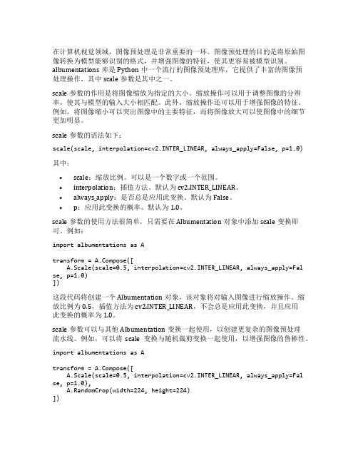
在计算机视觉领域,图像预处理是非常重要的一环。
图像预处理的目的是将原始图像转换为模型能够识别的格式,并增强图像的特征,使其更容易被模型识别。
albumentations库是Python中一个流行的图像预处理库,它提供了丰富的图像预处理操作,其中scale参数是其中之一。
scale参数的作用是将图像缩放为指定的大小。
缩放操作可以用于调整图像的分辨率,使其与模型的输入大小相匹配。
此外,缩放操作还可以用于增强图像的特征。
例如,将图像缩小可以突出图像中的主要特征,而将图像放大可以使图像中的细节更加明显。
scale参数的语法如下:scale(scale, interpolation=cv2.INTER_LINEAR, always_apply=False, p=1.0)其中:•scale:缩放比例。
可以是一个数字或一个范围。
•interpolation:插值方法。
默认为cv2.INTER_LINEAR。
•always_apply:是否总是应用此变换。
默认为False。
•p:应用此变换的概率。
默认为1.0。
scale参数的使用方法很简单,只需要在Albumentation对象中添加scale变换即可。
例如:import albumentations as Atransform = pose([A.Scale(scale=0.5, interpolation=cv2.INTER_LINEAR, always_apply=Fal se, p=1.0)])这段代码将创建一个Albumentation对象,该对象将对输入图像进行缩放操作。
缩放比例为0.5,插值方法为cv2.INTER_LINEAR,不会总是应用此变换,并且应用此变换的概率为1.0。
scale参数可以与其他Albumentation变换一起使用,以创建更复杂的图像预处理流水线。
例如,可以将scale变换与随机裁剪变换一起使用,以增强图像的鲁棒性。
import albumentations as Atransform = pose([A.Scale(scale=0.5, interpolation=cv2.INTER_LINEAR, always_apply=Fal se, p=1.0),A.RandomCrop(width=224, height=224)])这段代码将创建一个Albumentation对象,该对象将对输入图像进行缩放操作,然后随机裁剪图像。
- 1、下载文档前请自行甄别文档内容的完整性,平台不提供额外的编辑、内容补充、找答案等附加服务。
- 2、"仅部分预览"的文档,不可在线预览部分如存在完整性等问题,可反馈申请退款(可完整预览的文档不适用该条件!)。
- 3、如文档侵犯您的权益,请联系客服反馈,我们会尽快为您处理(人工客服工作时间:9:00-18:30)。
function img = My_read(path)
M=0;var=0;
I=double(imread(path));
[m,n,p]=size(I);
for x=1:m
for y=1:n
M=M+I(x,y);
end
end
M1=M/(m*n);
for x=1:m
for y=1:n
var=var+(I(x,y)-M1).^2;
end
end
var1=var/(m*n);
for x=1:m
for y=1:n
if I(x,y)>=M1
I(x,y)=150+sqrt(2000*(I(x,y)-M1)/var1); else
I(x,y)=150-sqrt(2000*(M1-I(x,y))/var1); end
end
end
figure, imshow(I(:,:,3)./max(max(I(:,:,3))));
title(‘归一化’)
M =3; %3*3
H = m/M;
L= n/M;
aveg1=zeros(H,L);
var1=zeros(H,L);
for x=1:H;
for y=1:L;
aveg=0;var=0;
for i=1:M;
for j=1:M;
aveg=I(i+(x-1)*M,j+(y-1)*M)+aveg; end
end
aveg1(x,y)=aveg/(M*M);
for i=1:M;
for j=1:M;
var=(I(i+(x-1)*M,j+(y-1)*M)-aveg1(x,y)).^2+var;
end
end
var1(x,y)=var/(M*M);
end
end
Gmean=0;
Vmean=0;
for x=1:H
for y=1:L
Gmean=Gmean+aveg1(x,y); Vmean=Vmean+var1(x,y);
end
end
Gmean1=Gmean/(H*L); %所有块的平均值Vmean1=Vmean/(H*L); %所有块的方差gtemp=0;
gtotle=0;
vtotle=0;
vtemp=0;
for x=1:H
for y=1:L
if Gmean1>aveg1(x,y)
gtemp=gtemp+1;
gtotle=gtotle+aveg1(x,y);
end
if Vmean1<var1(x,y)
vtemp=vtemp+1;
vtotle=vtotle+var1(x,y);
end
end
end
G1=gtotle/gtemp;
V1=vtotle/vtemp;
gtemp1=0;
gtotle1=0;
vtotle1=0;
vtemp1=0;
for x=1:H
for y=1:L
if G1<aveg1(x,y)
gtemp1=gtemp1-1;
gtotle1=gtotle1+aveg1(x,y);
End
if 0<var1(x,y)<V1
vtemp1=vtemp1+1;
vtotle1=vtotle1+var1(x,y);
end
end
End
G2=gtotle1/gtemp1;V2=vtotle1/vtemp1; e=zeros(H,L);
for x=1:H
for y=1:L
if aveg1(x,y)>G2 && var1(x,y)<V2
e(x,y)=1;
end
if aveg1(x,y)< G1-100 && var1(x,y)< V2
e(x,y)=1;
end
end
end
for x=2:H-1
for y=2:L-1
if e(x,y)==1
if e(x-1,y) + e(x-1,y+1) +e(x,y+1) + e(x+1,y+1) + e(x+1,y) + e(x+1,y-1) + e(x,y-1) + e(x-1,y-1) < =4
e(x,y)=0;
end
end
end
end
Icc = ones(m,n);
for x=1:H
for y=1:L
if e(x,y)==1
for i=1:M
for j=1:M
I(i+(x-1)*M,j+(y-1)*M)=G1;
Icc(i+(x-1)*M,j+(y-1)*M)=0;
end
end
end
end
end
figure, imshow(uint8(I));%title('分割');
temp=(1/9)*[1 1 1;1 1 1;1 1 1]; % 模板系数、均值滤波
Im=double(I); In=zeros(m,n);
for a=2:m-1;
for b=2:n-1;
In(a,b)=Im(a-1,b-1)*temp(1,1)+Im(a-1,b)*temp(1,2)+Im(a-1,b+1)*temp(1,3)+Im(a,b-1)*temp(2,1) +Im(a,b)*temp(2,2)+Im(a,b+1)*temp(2,3)+Im(a+1,b-1)*temp(3,1)+Im(a+1,b)*temp(3,2)+Im(a+1, b+1)*temp(3,3);
end
end
I=In;
Im=zeros(m,n);
for x=5:m-5;
for y=5:n-5;
sum1=I(x,y-4)+I(x,y-2)+I(x,y+2)+I(x,y+4);
sum2=I(x-2,y+4)+I(x-1,y+2)+I(x+1,y-2)+I(x+2,y-4);
sum3=I(x-2,y+2)+I(x-4,y+4)+I(x+2,y-2)+I(x+4,y-4);
sum4=I(x-2,y+1)+I(x-4,y+2)+I(x+2,y-1)+I(x+4,y-2);
sum5=I(x-2,y)+I(x-4,y)+I(x+2,y)+I(x+4,y);
sum6=I(x-4,y-2)+I(x-2,y-1)+I(x+2,y+1)+I(x+4,y+2);
sum7=I(x-4,y-4)+I(x-2,y-2)+I(x+2,y+2)+I(x+4,y+4);
sum8=I(x-2,y-4)+I(x-1,y-2)+I(x+1,y+2)+I(x+2,y+4);
sumi=[sum1,sum2,sum3,sum4,sum5,sum6,sum7,sum8];
summax=max(sumi);
summin=min(sumi);
summ=sum(sumi);
b=summ/8;
if (summax+summin+ 4*I(x,y))> (3*summ/8)
sumf = summin;
else
sumf =summax;
end
if sumf > b
Im(x,y)=128;
else
Im(x,y)=255;
end
end
end
for i=1:m
for j =1:n
Icc(i,j)=Icc(i,j)*Im(i,j);
end
end
for i=1:m
for j =1:n
if (Icc(i,j)==128)
Icc(i,j)=0;
else
Icc(i,j)=1;
end;
end
end
figure,imshow(double(Icc));title('二值化');
u=Icc;
for a=2:m-1
for b=2:n-1
if u(a,b)==1
if abs(u(a,b+1)-u(a-1,b+1))+abs(u(a-1,b+1)-u(a-1,b))+abs(u(a-1,b)-u(a-1,b-1))+abs(u(a-1,b-1)-u(a,b -1))+abs(u(a,b-1)-u(a+1,b-1))+abs(u(a+1,b-1)-u(a+1,b))+abs(u(a+1,b)-u(a+1,b+1))+abs(u(a+1,b+1)-u(a,b+1))~=1 ;%去空洞
if(u(a,b+1)+u(a-1,b+1)+u(a-1,b))*(u(a,b-1)+u(a+1,b-1)+u(a+1,b))+(u(a-1,b)+u(a-1,b-1)+u(a,b-1))*( u(a+1,b)+u(a+1,b+1)+u(a,b+1))==0 %去毛刺
u(a,b)=0;
end
end
end
end
end
figure,imshow(u);%title('去空洞')。