Bootstrap Approach for Estimating Seemingly Unrelated Regressions with Varying Degrees

合集下载

关于bootstrap的思想的讨论

关于bootstrap的思想的讨论1楼rtist看了/view.php?tid=48&id=86之后想留言，可是那里不让留了，就贴在这儿了。

bootstrap的思想并不是再抽样，而是plug-in principle；再抽样仅仅是实现这个思想的一种手段。

所以bootstrap也并不一定非要抽样B次，只要可以plug-in，有时候一次也不用抽就可以得到精确结果。

但是不可否认，样本的重复利用的确是一个incredibly amazing的方法，而且经常counter-intuitive。

最难理解的（对我来说）就是，信息都蕴含在样本中，再抽样究竟能提不提供样本之外的新的信息；如果不能，怎么抽得到的都是原来样本里面的信息；如果能，新信息从哪儿来？2楼keynesI think the information contained in a sample is not always fully exploited by a particular statistic. That is, a statistic typically only uses part of information in the data and the principle of data-reduction is one of such examples. To use bootstrap (maybe other resampling methods as well), we have to impose some extra assumptions, such like the sample (the data at hand, so to speak) is representative and informative of the population so that we can treat the former as the latter.Not quite clear what do you mean by the statement that the bootstrap is mainly a plug-in method. Would you make it more clear and detailed? Thanks.3楼rtistI don't think so, as bootstrap often works on complete sufficient statistics too. So it's not that the original statistic always loses information that allows bootstrap to exploit further.It's still counter-intuitive to me. My current understanding (subject to change in the future) is that we often make reasonable assumptions that give us the extra-information, so that bootstrap often works by using the information in the assumptions.For the plug-in principle, see Efron's review: /view/08834237/sp040007/04x0072t/04楼keynesWell, "sufficient" just means that the statistic contain enough information for the purpose of point estimation of the parameter of interest. It does not say that all information is used up. Neither it prevents from exploiting other information contained in the sample.5楼rtistThis is also point that I was thinking of when I was writing the last post.It sounds reasonable, but it didn't completely persuade me to believe it at the timeas I could not figure out just what is the "other" information. Are we treating the sd ofsome statistic as a new parameter to estimate? Probably.6楼statax我也一直觉得这个问题很玄乎。

No1【方法学导读】SPSS和SAS在简单中介模型中间接效应估计中的应用(中文译校)

推荐序中介分析的初衷在于揭示变量间作用的“机制”，最简单的完全中介模型就是包含一个中介变量的模型，即X→M→Y。

在中国知网平台《心理学报》发表论文的初步内容分析发现，2000年以来涉及“中介”分析的论文发表数量呈缓慢增长趋势，特别是，2016年以来每年约10篇左右的论文涉及到“中介”分析。

在众多探讨中介方法的中文文献中，尤其以温忠麟、侯杰泰、张雷老师合作发表的《中介效应检验程序及其应用》、《调节效应与中介效应的比较和应用》两篇文章最为引人注目，引用率高达8000余次，对于推动国内心理学界更多、更正式地使用中介分析做出了有目共睹的贡献。

这种趋势还是继续。

国内有限的几本发表实证研究的期刊，再也很难看到没有中介调节分析而能发表的非实验类、非综述类的文章了。

据初步估计，本校心理学本科生的论文中70%左右有用到中介分析，而心理学硕士学位论文使用中介分析的比例几乎高达90%，但用错、报告错、得出奇怪结论的情况总是难免，但研究者有时不自知、他人也不容易发现。

这当中，所引用的外文文献都比较一致地指向2004年发表于的一篇文章：《SPSS and SAS procedures for estimating indirect effects in simple mediation models》，引用率已突破6000次，这其中可能还不包括规模庞大的中文期刊论文以及中国学士以上学位论文引用的人数。

个人推测，这篇文章最受欢迎之处在于它提供了傻瓜式的宏。

然而，真正阅读英文原文的本科生和研究生人数可能并不乐观，老师们也未必能有雅兴拜读这篇原文。

本次推介的目的，反而并不是要介绍“宏”，而是尽量准确地翻译作者开发宏背后的“理”；误差也是难免的，请大家指正，是为序。

SPSS和SAS宏程序在简单中介模型的间接效应估计中的应用KRISTOPHER J. PREACHER北卡罗来纳大学ANDREW F . HAYES俄亥俄州立大学摘要：中介分析（mediation analysis）常用来间接评估假设的某个原因是否通过中介变量（mediator）对结果产生影响。

健康预期寿命的测量指标与测算方法的应用及比较

健康预期寿命的测量指标与测算方法的应用及比较厦门大学公共卫生学院(361002)展元元韩耀风方亚*【中图分类号】R3 【文献标识码】A DOI 10. 3969/j.issn. 1002 -3674. 2020.06.002健康预期寿命(health expectancy , HE )是一项结合预期寿命与健康状态以反映人群生命质量的综合性指标。

面对快速老龄化、疾病模式的转变等带来的一系列负担与挑战,2016年10月25日，国务院公布的《“健康中国2030”规划纲要》提出“到2030年预期寿命达到79.0岁,健康预期寿命显著提高”。

美国和欧盟等国家早已将HE 作为政策目标［1］，可见提高人类HE 已成为国际关注的焦点。

然而，由于HE 测量指标与测算方法的复杂性与多样性，《“健康中国2030”规划纲要》并没有明确具体的健康预期寿命政策目标值。

虽然国内有学者已对HE 的概念、理论框架、测算方法等作了较为详细的论述［1-3］,但对HE测量指标和测算方法在实际应用中的适用性仍缺乏明确、详细的指导与说明。

因此,本文从适用性角度对HE 的测量指标和测算方法进行综述，旨在为HE 的测量指标和测算方法在实际应用中的恰当选择提供参考。

△通信作者:方亚,E-mail : fangya@ xum. edu. cn健康预期寿命的测量指标自1964年Sanders 首次将伤残的概念引入预期寿命后,HE 指标日趋多样化。

2002年，国际健康预期寿命研究网络的核心成员Robine 根据是否按权重调整将健康预期寿命分为健康调整预期寿命(health adjusted life expectancy ,HALE )和健康状态预期寿命(health state expectancy , HSE )［1］ o1.健康调整预期寿命HALE 主要包括伤残调整预期寿命(disability adj u sted life expectancy ,DALE )和质量调整预期寿命(quality-adjusted life expectancy , QALE ) 2 类。

[转载]k-折交叉验证（K-fold

[转载]k-折交叉验证（K-fold cross-validation）原⽂地址：k-折交叉验证（K-fold cross-validation）作者：清风⼩荷塘k-折交叉验证（K-fold cross-validation）是指将样本集分为k份，其中k-1份作为训练数据集，⽽另外的1份作为验证数据集。

⽤验证集来验证所得分类器或者回归的错误码率。

⼀般需要循环k次，直到所有k份数据全部被选择⼀遍为⽌。

Cross validation is a model evaluation method that is better than residuals. The problem with residual evaluations is that they do not give an indication of how well the learner will do when it is asked to make new predictions for data it has not already seen. One way to overcome this problem is to not use the entire data set when training a learner. Some of the data is removed before training begins. Then when training is done, the data that was removed can be used to test the performance of the learned model on ``new'' data. This is the basic idea for a whole class of model evaluation methods called cross validation.The holdout method is the simplest kind of cross validation. The data set is separated into two sets, called the training set and the testing set. The function approximator fits a function using the training set only. Then the function approximator is asked to predict the output values for the data in the testing set (it has never seen these output values before). The errors it makes are accumulated as before to give the mean absolute test set error, which is used to evaluate the model. The advantage of this method is that it is usually preferable to the residual method and takes no longer to compute. However, its evaluation can have a high variance. The evaluation may depend heavily on which data points end up in the training set and which end up in the test set, and thus the evaluation may be significantly different depending on how the division is made.K-fold cross validation is one way to improve over the holdout method. The data set is divided into k subsets, and the holdout method is repeated k times. Each time, one of the k subsets is used as the test set and the other k-1 subsets are put together to form a training set. Then the average error across all k trials is computed. The advantage of this method is that it matters less how the data gets divided. Every data point gets to be in a test set exactly once, and gets to be in a training set k-1 times. The variance of the resulting estimate is reduced as k is increased. The disadvantage of this method is that the training algorithm has to be rerun from scratch k times, which means it takes k times as much computation to make an evaluation. A variant of this method is to randomly divide the data into a test and training set k different times. The advantage of doing this is that you can independently choose how large each test set is and how many trials you average over.Leave-one-out cross validation is K-fold cross validation taken to its logical extreme, with K equal to N, the number of da ta points in the set. That means that N separate times, the function approximator is trained on all the data except for one point and a prediction is made for that point. As before the average error is computed and used to evaluate the model. The evaluation given by leave-one-out cross validation error (LOO-XVE) is good, but at first pass it seems very expensive to compute. Fortunately, locally weighted learners can make LOO predictions just as easily as they make regular predictions. That means computing the LOO-XVE takes no more time than computing the residual error and it is a much better way to evaluate models. We will see shortly that Vizier relies heavily on LOO-XVE to choose its metacodes.Figure 26: Cross validation checks how well a model generalizes to new dataFig. 26 shows an example of cross validation performing better than residual error. The data set in the top two graphs is a simple underlying function with significant noise. Cross validation tells us that broad smoothing is best. The data set in the bottom two graphs is a complex underlying function with no noise. Cross validation tells us that very little smoothing is best for this data set.Now we return to the question of choosing a good metacode for data set a1.mbl:File -> Open -> a1.mblEdit -> Metacode -> A90:9Model -> LOOPredictEdit -> Metacode -> L90:9Model -> LOOPredictEdit -> Metacode -> L10:9Model -> LOOPredictLOOPredict goes through the entire data set and makes LOO predictions for each point. At the bottom of the page itshows the summary statistics including Mean LOO error, RMS LOO error, and information about the data point with the largest error. The mean absolute LOO-XVEs for the three metacodes given above (the same three used to generate the graphs in fig. 25), are 2.98, 1.23, and 1.80. Those values show that global linear regression is the best metacode of those three, which agrees with our intuitive feeling from looking at the plots in fig. 25. If you repeat the above operation on data set b1.mbl you'll get the values 4.83, 4.45, and 0.39, which also agrees with our observations.What are cross-validation and bootstrapping?--------------------------------------------------------------------------------Cross-validation and bootstrapping are both methods for estimatinggeneralization error based on "resampling" (Weiss and Kulikowski 1991; Efronand Tibshirani 1993; Hjorth 1994; Plutowski, Sakata, and White 1994; Shaoand Tu 1995). The resulting estimates of generalization error are often usedfor choosing among various models, such as different network architectures.Cross-validation++++++++++++++++In k-fold cross-validation, you divide the data into k subsets of(approximately) equal size. You train the net k times, each time leavingout one of the subsets from training, but using only the omitted subset tocompute whatever error criterion interests you. If k equals the samplesize, this is called "leave-one-out" cross-validation. "Leave-v-out" is amore elaborate and expensive version of cross-validation that involvesleaving out all possible subsets of v cases.Note that cross-validation is quite different from the "split-sample" or"hold-out" method that is commonly used for early stopping in NNs. In thesplit-sample method, only a single subset (the validation set) is used toestimate the generalization error, instead of k different subsets; i.e.,there is no "crossing". While various people have suggested thatcross-validation be applied to early stopping, the proper way of doing so isnot obvious.The distinction between cross-validation and split-sample validation isextremely important because cross-validation is markedly superior for smalldata sets; this fact is demonstrated dramatically by Goutte (1997) in areply to Zhu and Rohwer (1996). For an insightful discussion of thelimitations of cross-validatory choice among several learning methods, seeStone (1977).Jackknifing+++++++++++Leave-one-out cross-validation is also easily confused with jackknifing.Both involve omitting each training case in turn and retraining the networkon the remaining subset. But cross-validation is used to estimategeneralization error, while the jackknife is used to estimate the bias of astatistic. In the jackknife, you compute some statistic of interest in eachsubset of the data. The average of these subset statistics is compared withthe corresponding statistic computed from the entire sample in order toestimate the bias of the latter. You can also get a jackknife estimate ofthe standard error of a statistic. Jackknifing can be used to estimate thebias of the training error and hence to estimate the generalization error,but this process is more complicated than leave-one-out cross-validation(Efron, 1982; Ripley, 1996, p. 73).Choice of cross-validation method+++++++++++++++++++++++++++++++++Cross-validation can be used simply to estimate the generalization error of a given model, or it can be used for model selection by choosing one of several models that has the smallest estimated generalization error. For example, you might use cross-validation to choose the number of hidden units, or you could use cross-alidation to choose a subset of the inputs (subset selection). A subset that contains all relevant inputs will be called a "good" subsets, while the subset that contains all relevant inputs but no others will be called the "best" subset. Note that subsets are "good" and "best" in an asymptotic sense (as the number of training cases goes to infinity). With a small training set, it is possible that a subset that is smaller than the "best" subset may provide better generalization error.Leave-one-out cross-validation often works well for estimating generalization error for continuous error functions such as the mean squared error, but it may perform poorly for discontinuous error functions such as the number of misclassified cases. In the latter case, k-fold cross-validation is preferred. But if k gets too small, the error estimate is pessimistically biased because of the difference in training-set size between the full-sample analysis and the cross-validation analyses. (For model-selection purposes, this bias can actually help; see the discussion below of Shao, 1993.) A value of 10 for k is popular for estimating generalization error.Leave-one-out cross-validation can also run into trouble with variousmodel-selection methods. Again, one problem is lack of continuity--a smallchange in the data can cause a large change in the model selected (Breiman,1996). For choosing subsets of inputs in linear regression, Breiman andSpector (1992) found 10-fold and 5-fold cross-validation to work better thanleave-one-out. Kohavi (1995) also obtained good results for 10-foldcross-validation with empirical decision trees (C4.5). Values of k as smallas 5 or even 2 may work even better if you analyze several different randomk-way splits of the data to reduce the variability of the cross-validationestimate.Leave-one-out cross-validation also has more subtle deficiencies for modelselection. Shao (1995) showed that in linear models, leave-one-outcross-validation is asymptotically equivalent to AIC (and Mallows' C_p), butleave-v-out cross-validation is asymptotically equivalent to Schwarz's Bayesian criterion (called SBC or BIC) when v =n[1-1/(log(n)-1)], where n is the number of training cases. SBCprovides consistent subset-selection, while AIC does not. That is, SBC will choose the "best" subset with probability approaching one as the size of the training set goes to infinity. AIC has an asymptotic probability of one of choosing a "good" subset, but less than one of choosing the "best" subset (Stone, 1979). Many simulation studies have also found that AIC overfits badly in small samples, and that SBC works well (e.g., Hurvich and Tsai, 1989; Shao and Tu, 1995). Hence, these results suggest that leave-one-out cross-validation should overfit in small samples, but leave-v-outcross-validation with appropriate v should do better. However, when true models have an infinite number of parameters, SBC is not efficient, and other criteria that are asymptotically efficient but not consistent formodel selection may produce better generalization (Hurvich and Tsai, 1989). Shao (1993) obtained the surprising result that for selecting subsets of inputs in a linear regression, the probability of selecting the "best" doesnot converge to 1 (as the sample size n goes to infinity) for leave-v-out cross-validation unless the proportion v/n approaches 1. At first glance, Shao's result seems inconsistent with the analysis by Kearns (1997) ofsplit-sample validation, which shows that the best generalization is obtained with v/n strictly between 0 and 1, with little sensitivity to the precise value of v/n for large data sets. But the apparent conflict is dueto the fundamentally different properties of cross-validation andsplit-sample validation.To obtain an intuitive understanding of Shao (1993), let's review some background material on generalization error. Generalization error can be broken down into three additive parts, noise variance + estimation variance + squared estimation bias. Noise variance is the same for all subsets of inputs. Bias is nonzero for subsets that are not "good", but it's zero forall "good" subsets, since we are assuming that the function to be learned is linear. Hence the generalization error of "good" subsets will differ only in the estimation variance. The estimation variance is (2p/t)s^2 where pis the number of inputs in the subset, t is the training set size, and s^2is the noise variance. The "best" subset is better than other "good" subsetsonly because the "best" subset has (by definition) the smallest value of p. But the t in the denominator means that differences in generalization error among the "good" subsets will all go to zero as t goes to infinity.Therefore it is difficult to guess which subset is "best" based on the generalization error even when t is very large. It is well known that unbiased estimates of the generalization error, such as those based on AIC, FPE, and C_p, do not produce consistent estimates of the "best" subset (e.g., see Stone, 1979).In leave-v-out cross-validation, t=n-v. The differences of thecross-validation estimates of generalization error among the "good" subsets contain a factor 1/t, not 1/n. Therefore by making t small enough (and thereby making each regression based on t cases bad enough), we can make the differences of the cross-validation estimates large enough to detect. It turns out that to make t small enough to guess the "best" subset consistently, we have to have t/n go to 0 as n goes to infinity.The crucial distinction between cross-validation and split-sample validation is that with cross-validation, after guessing the "best" subset, we trainthe linear regression model for that subset using all n cases, but withsplit-sample validation, only t cases are ever used for training. If ourmain purpose were really to choose the "best" subset, I suspect we would still have to have t/n go to 0 even for split-sample validation. Butchoosing the "best" subset is not the same thing as getting the best generalization. If we are more interested in getting good generalizationthan in choosing the "best" subset, we do not want to make our regression estimate based on only t cases as bad as we do in cross-validation, because in split-sample validation that bad regression estimate is what we're stuck with. So there is no conflict between Shao and Kearns, but there is a conflict between the two goals of choosing the "best" subset and getting the best generalization in split-sample validation.Bootstrapping+++++++++++++Bootstrapping seems to work better than cross-validation in many cases (Efron, 1983). In the simplest form of bootstrapping, instead of repeatedly analyzing subsets of the data, you repeatedly analyze subsamples of the data. Each subsample is a random sample with replacement from the fullsample. Depending on what you want to do, anywhere from 50 to 2000 subsamples might be used. There are many more sophisticated bootstrap methods that can be used not only for estimating generalization error butalso for estimating confidence bounds for network outputs (Efron and Tibshirani 1993). For estimating generalization error in classification problems, the .632+ bootstrap (an improvement on the popular .632 bootstrap) is one of the currently favored methods that has the advantage of performing well even when there is severe overfitting. Use of bootstrapping for NNs is described in Baxt and White (1995), Tibshirani (1996), and Masters (1995). However, the results obtained so far are not very thorough, and it is known that bootstrapping does not work well for some other methodologies such as empirical decision trees (Breiman, Friedman, Olshen, and Stone, 1984; Kohavi, 1995), for which it can be excessively optimistic.For further information+++++++++++++++++++++++Cross-validation and bootstrapping become considerably more complicated for time series data; see Hjorth (1994) and Snijders (1988).More information on jackknife and bootstrap confidence intervals is available at ftp:///pub/neural/jackboot.sas (this is a plain-text file).References:Baxt, W.G. and White, H. (1995) "Bootstrapping confidence intervals forclinical input variable effects in a network trained to identify thepresence of acute myocardial infarction", Neural Computation, 7, 624-638. Breiman, L., and Spector, P. (1992), "Submodel selection and evaluationin regression: The X-random case," International Statistical Review, 60,291-319.Dijkstra, T.K., ed. (1988), On Model Uncertainty and Its StatisticalImplications, Proceedings of a workshop held in Groningen, TheNetherlands, September 25-26, 1986, Berlin: Springer-Verlag.Efron, B. (1982) The Jackknife, the Bootstrap and Other ResamplingPlans, Philadelphia: SIAM.Efron, B. (1983), "Estimating the error rate of a prediction rule:Improvement on cross-validation," J. of the American StatisticalAssociation, 78, 316-331.Efron, B. and Tibshirani, R.J. (1993), An Introduction to the Bootstrap,London: Chapman & Hall.Efron, B. and Tibshirani, R.J. (1997), "Improvements on cross-validation: The .632+ bootstrap method," J. of the American Statistical Association, 92, 548-560.Goutte, C. (1997), "Note on free lunches and cross-validation," NeuralComputation, 9, 1211-1215,ftp://eivind.imm.dtu.dk/dist/1997/goutte.nflcv.ps.gz.Hjorth, J.S.U. (1994), Computer Intensive Statistical Methods Validation, Model Selection, and Bootstrap, London: Chapman & Hall.Hurvich, C.M., and Tsai, C.-L. (1989), "Regression and time series model selection in small samples," Biometrika, 76, 297-307.Kearns, M. (1997), "A bound on the error of cross validation using theapproximation and estimation rates, with consequences for thetraining-test split," Neural Computation, 9, 1143-1161.Kohavi, R. (1995), "A study of cross-validation and bootstrap foraccuracy estimation and model selection," International Joint Conference on Artificial Intelligence (IJCAI), pp. ?,/users/ronnyk/Masters, T. (1995) Advanced Algorithms for Neural Networks: A C++Sourcebook, NY: John Wiley and Sons, ISBN 0-471-10588-0Plutowski, M., Sakata, S., and White, H. (1994), "Cross-validationestimates IMSE," in Cowan, J.D., Tesauro, G., and Alspector, J. (eds.)Advances in Neural Information Processing Systems 6, San Mateo, CA: Morgan Kaufman, pp. 391-398.Ripley, B.D. (1996) Pattern Recognition and Neural Networks, Cambridge: Cambridge University Press.Shao, J. (1993), "Linear model selection by cross-validation," J. of theAmerican Statistical Association, 88, 486-494.Shao, J. (1995), "An asymptotic theory for linear model selection,"Statistica Sinica ?.Shao, J. and Tu, D. (1995), The Jackknife and Bootstrap, New York:Springer-Verlag.Snijders, T.A.B. (1988), "On cross-validation for predictor evaluation intime series," in Dijkstra (1988), pp. 56-69.Stone, M. (1977), "Asymptotics for and against cross-validation,"Biometrika, 64, 29-35.Stone, M. (1979), "Comments on model selection criteria of Akaike and Schwarz," J. of the Royal Statistical Society, Series B, 41, 276-278.Tibshirani, R. (1996), "A comparison of some error estimates for neural network models," Neural Computation, 8, 152-163.Weiss, S.M. and Kulikowski, C.A. (1991), Computer Systems That Learn, Morgan Kaufmann.Zhu, H., and Rohwer, R. (1996), "No free lunch for cross-validation,"Neural Computation, 8, 1421-1426.。

bootstrap置信区间公式

bootstrap置信区间公式## Confidence Intervals for Means Using Bootstrapping.Introduction.Bootstrapping is a technique used to estimatestatistical parameters, such as confidence intervals, by resampling a given dataset with replacement. For example, to calculate a confidence interval for the mean of a population, bootstrapping involves repeatedly sampling from the original dataset, calculating the mean of each sample, and then using the distribution of these sample means to estimate the population mean and the associated confidence interval.Formula.The basic formula for a bootstrap confidence interval for the mean using the percentile method is:CI = (L, U)。

where:L is the lower bound of the confidence interval, which is the _p_th percentile of the sample means, where _p_ is the desired level of confidence.U is the upper bound of the confidence interval, which is the _q_th percentile of the sample means, where _q_ is 1 _p_.For example, if we want a 95% confidence interval, then _p_ = 0.025 and _q_ = 0.975.Steps.The steps for calculating a bootstrap confidence interval for the mean are as follows:1. Resample: Draw B bootstrap samples of size n from the original dataset with replacement.2. Calculate: Compute the mean for each bootstrap sample.3. Percentile: Determine the lower and upper bounds of the confidence interval by finding the _p_th and _q_th percentiles of the sample means.4. Confidence Interval: The interval (L, U) is the bootstrap confidence interval for the mean.Advantages.Bootstrapping has several advantages over traditional methods for estimating confidence intervals, such as:It is non-parametric, so it does not require assumptions about the distribution of the data.It can be used with small sample sizes.It is computationally efficient and easy to implement.Limitations.However, bootstrapping also has some limitations:It can be biased for certain types of data or if the sample size is too small.It can be computationally intensive for large datasets.It may not be accurate if the data is notrepresentative of the population.## 置信区间公式。

基于Bootstrap方法数据包络分析的回归分析_全林(1)

1、U 2、U 3、U 4和 U 5) SC AL E 和 N AV (其系数分别为 U 2 2
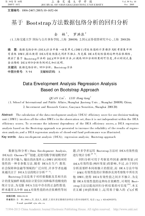
θ j = U 0+ U 1 F1j + U 2 F2j + … + U q Fqj Fs 的回归系数 ; j = 1, 2, … , n .
( 2)
式中 : U 0 为回归截距 ; U s ( s = 1, 2, … , q )为解释变量 ( 2) 利用配对 Boot strap 方法 , 有放回地从原样本 ( z 1 , z 2 ,… , z n )中随机抽取 c (常数 )个 n 维样本 , 产生所谓的 Bo ot st rap 样本 Sk : Sk = ( z k 1 , zk 2 , … , z kn ) k = 1, 2, … , c zk j = ( ukj , v kj ) ( 3) 对每一 Boo tst rap 样本 Sk , 运行 C GS 模型 , 重新计算所有 n 个 DM U 的有效性值 θ k1 , θ k2 , … ,θ kn . ( 4) 在每一 Boo tst rap 样本 Sk 内 , 拟合模型 :
2 ห้องสมุดไป่ตู้实例
以 2000 年前上市的 20 只封闭式基金 2000 年 ( 1) 业绩为考察对象 (即 n = 20) , 所采用的输入指标为管理费用 ( M FP U)、交易成本 ( T CPU ) 和标准差 ( SD ) , 输出指标则为基金收益率 . 其中 , M F PU (不包括基金经理业绩报酬 )、 T CPU (用年佣金总计代替 , 即显性交易成本 )均折算为每单位基金的数值 (单位为元 ) , SD指的是评价期内基金周收益率的标准差 , 基金周收益率计算公式为 Rit = ln N AVit + Dit N AVi , t - 1 ( 5)

bootstrap法

bootstrap法Bootstrap法是一种常用的统计学方法，它可以用来评估统计学中的参数估计和假设检验的准确性。

Bootstrap法最初由布拉德利·埃夫隆和皮特·哈尔在1979年提出，并在之后的几十年里得到了广泛的应用。

本文将介绍Bootstrap法的基本原理、应用场景以及实现方法。

一、Bootstrap法的原理Bootstrap法的基本思想是通过从样本中重复抽取数据来估计统计量的分布。

具体而言，Bootstrap法包括以下步骤：1. 从原始数据样本中随机抽取一个固定数量的样本（通常与原始样本大小相同），并将其作为一个新的样本。

2. 重复步骤1多次，通常是1000次或更多次。

3. 对每个新样本计算统计量（如均值、方差、中位数等）。

4. 将所有计算出的统计量按升序排列。

5. 根据需要计算出置信区间和标准误等统计量。

Bootstrap法的核心在于重复抽样。

通过从原始数据样本中重复随机抽样，我们可以获得更准确的统计量估计和假设检验结果。

在某些情况下，原始数据可能不符合正态分布或其他假设检验的前提条件。

Bootstrap法可以通过生成新的样本来解决这些问题。

二、Bootstrap法的应用场景Bootstrap法可以用于各种统计学应用中，包括参数估计、假设检验、回归分析、时间序列分析等。

以下是Bootstrap法的一些常见应用场景：1. 参数估计：Bootstrap法可以用来估计统计量的标准误和置信区间，如均值、中位数、方差、相关系数等。

2. 假设检验：Bootstrap法可以用来检验假设检验的显著性，如两个总体均值是否相等、回归系数是否显著等。

3. 回归分析：Bootstrap法可以用来估计回归系数的标准误和置信区间，以及模型的预测误差等。

4. 时间序列分析：Bootstrap法可以用来估计时间序列模型的参数和预测误差，以及分析时间序列的置信区间和假设检验结果等。

三、Bootstrap法的实现方法Bootstrap法的实现方法相对简单，可以使用各种编程语言和软件包来实现。

用MATLAB的时重要MATLAB tools

用MATLAB的时重要MATLAB toolsADCPtools - acoustic doppler current profiler data processingAFDesign - designing analog and digital filtersAIRES - automatic integration of reusable embedded softwareAir-Sea - air-sea flux estimates in oceanographyAnimation - developing scientific animationsARfit - estimation of parameters and eigenmodes of multivariate autoregressive methodsARMASA - power spectrum estimationAR-Toolkit - computer vision trackingAuditory - auditory modelsb4m - interval arithmeticBayes Net - inference and learning for directed graphical modelsBinaural Modeling - calculating binaural cross-correlograms of soundBode Step - design of control systems with maximized feedbackBootstrap - for resampling, hypothesis testing and confidence interval estimationBrainStorm - MEG and EEG data visualization and processingBSTEX - equation viewerCALFEM - interactive program for teaching the finite element methodCalibr - for calibrating CCD camerasCamera CalibrationCaptain - non-stationary time series analysis and forecastingCHMMBOX - for coupled hidden Markov modeling using maximum likelihood EM Classification - supervised and unsupervised classification algorithmsCLOSIDCluster - for analysis of Gaussian mixture models for data set clusteringClustering - cluster analysisClusterPack - cluster analysisCOLEA - speech analysisCompEcon - solving problems in economics and financeComplex - for estimating temporal and spatial signal complexitiesComputational StatisticsCoral - seismic waveform analysisDACE - kriging approximations to computer modelsDAIHM - data assimilation in hydrological and hydrodynamic modelsData VisualizationDBT - radar array processingDDE-BIFTOOL - bifurcation analysis of delay differential equationsDenoise - for removing noise from signalsDiffMan - solving differential equations on manifoldsDimensional Analysis -DIPimage - scientific image processingDirect - Laplace transform inversion via the direct integration methodDirectSD - analysis and design of computer controlled systems with process-oriented modelsDMsuite - differentiation matrix suiteDMTTEQ - design and test time domain equalizer design methodsDrawFilt - drawing digital and analog filtersDSFWAV - spline interpolation with Dean wave solutionsDWT - discrete wavelet transformsEasyKrigEconometricsEEGLABEigTool - graphical tool for nonsymmetric eigenproblemsEMSC - separating light scattering and absorbance by extended multiplicative signal correctionEngineering VibrationFastICA - fixed-point algorithm for ICA and projection pursuitFDC - flight dynamics and controlFDtools - fractional delay filter designFlexICA - for independent components analysisFMBPC - fuzzy model-based predictive controlForWaRD - Fourier-wavelet regularized deconvolutionFracLab - fractal analysis for signal processingFSBOX - stepwise forward and backward selection of features using linear regressionGABLE - geometric algebra tutorialGAOT - genetic algorithm optimizationGarch - estimating and diagnosing heteroskedasticity in time series modelsGCE Data - managing, analyzing and displaying data and metadata stored using the GCE data structure specificationGCSV - growing cell structure visualizationGEMANOVA - fitting multilinear ANOVA modelsGenetic AlgorithmGeodetic - geodetic calculationsGHSOM - growing hierarchical self-organizing mapglmlab - general linear modelsGPIB - wrapper for GPIB library from National InstrumentGTM - generative topographic mapping, a model for density modeling and data visualizationGVF - gradient vector flow for finding 3-D object boundariesHFRadarmap - converts HF radar data from radial current vectors to total vectorsHFRC - importing, processing and manipulating HF radar dataHilbert - Hilbert transform by the rational eigenfunction expansion methodHMM - hidden Markov modelsHMMBOX - for hidden Markov modeling using maximum likelihood EMHUTear - auditory modelingICALAB - signal and image processing using ICA and higher order statisticsImputation - analysis of incomplete datasetsIPEM - perception based musical analysisJMatLink - Matlab Java classesKalman - Bayesian Kalman filterKalman Filter - filtering, smoothing and parameter estimation (using EM) for linear dynamical systemsKALMTOOL - state estimation of nonlinear systemsKautz - Kautz filter designKrigingLDestimate - estimation of scaling exponentsLDPC - low density parity check codesLISQ - wavelet lifting scheme on quincunx gridsLKER - Laguerre kernel estimation toolLMAM-OLMAM - Levenberg Marquardt with Adaptive Momentum algorithm for training feedforward neural networksLow-Field NMR - for exponential fitting, phase correction of quadrature data and slicingLPSVM - Newton method for LP support vector machine for machine learning problemsLSDPTOOL - robust control system design using the loop shaping design procedure LS-SVMlabLSVM - Lagrangian support vector machine for machine learning problemsLyngby - functional neuroimagingMARBOX - for multivariate autogressive modeling and cross-spectral estimationMatArray - analysis of microarray dataMatrix Computation - constructing test matrices, computing matrix factorizations, visualizing matrices, and direct search optimizationMCAT - Monte Carlo analysisMDP - Markov decision processesMESHPART - graph and mesh partioning methodsMILES - maximum likelihood fitting using ordinary least squares algorithmsMIMO - multidimensional code synthesisMissing - functions for handling missing data valuesM_Map - geographic mapping toolsMODCONS - multi-objective control system designMOEA - multi-objective evolutionary algorithmsMS - estimation of multiscaling exponentsMultiblock - analysis and regression on several data blocks simultaneouslyMultiscale Shape AnalysisMusic Analysis - feature extraction from raw audio signals for content-based music retrievalMWM - multifractal wavelet modelNetCDFNetlab - neural network algorithmsNiDAQ - data acquisition using the NiDAQ libraryNEDM - nonlinear economic dynamic modelsNMM - numerical methods in Matlab textNNCTRL - design and simulation of control systems based on neural networksNNSYSID - neural net based identification of nonlinear dynamic systemsNSVM - newton support vector machine for solving machine learning problemsNURBS - non-uniform rational B-splinesN-way - analysis of multiway data with multilinear modelsOpenFEM - finite element developmentPCNN - pulse coupled neural networksPeruna - signal processing and analysisPhiVis - probabilistic hierarchical interactive visualization, i.e. functions for visual analysis of multivariate continuous dataPlanar Manipulator - simulation of n-DOF planar manipulatorsPRTools - pattern recognitionpsignifit - testing hyptheses about psychometric functionsPSVM - proximal support vector machine for solving machine learning problemsPsychophysics - vision researchPyrTools - multi-scale image processingRBF - radial basis function neural networksRBN - simulation of synchronous and asynchronous random boolean networksReBEL - sigma-point Kalman filtersRegression - basic multivariate data analysis and regressionRegularization ToolsRegularization Tools XPRestore ToolsRobot - robotics functions, e.g. kinematics, dynamics and trajectory generationRobust Calibration - robust calibration in statsRRMT - rainfall-runoff modellingSAM - structure and motionSchwarz-Christoffel - computation of conformal maps to polygonally bounded regions SDH - smoothed data histogramSeaGrid - orthogonal grid makerSEA-MAT - oceanographic analysisSLS - sparse least squaresSolvOpt - solver for local optimization problemsSOM - self-organizing mapSOSTOOLS - solving sums of squares (SOS) optimization problemsSpatial and Geometric AnalysisSpatial RegressionSpatial StatisticsSpectral MethodsSPM - statistical parametric mappingSSVM - smooth support vector machine for solving machine learning problemsSTATBAG - for linear regression, feature selection, generation of data, and significance testingStatBox - statistical routinesStatistical Pattern Recognition - pattern recognition methodsStixbox - statisticsSVM - implements support vector machinesSVM ClassifierSymbolic Robot DynamicsTEMPLAR - wavelet-based template learning and pattern classificationTextClust - model-based document clusteringTextureSynth - analyzing and synthesizing visual texturesTfMin - continous 3-D minimum time orbit transfer around EarthTime-Frequency - analyzing non-stationary signals using time-frequency distributions Tree-Ring - tasks in tree-ring analysisTSA - uni- and multivariate, stationary and non-stationary time series analysisTSTOOL - nonlinear time series analysisT_Tide - harmonic analysis of tidesUTVtools - computing and modifying rank-revealing URV and UTV decompositions Uvi_Wave - wavelet analysisvarimax - orthogonal rotation of EOFsVBHMM - variation Bayesian hidden Markov modelsVBMFA - variational Bayesian mixtures of factor analyzersVMT - VRML Molecule Toolbox, for animating results from molecular dynamics experimentsVOICEBOXVRMLplot - generates interactive VRML 2.0 graphs and animationsVSVtools - computing and modifying symmetric rank-revealing decompositionsWAFO - wave analysis for fatique and oceanographyWarpTB - frequency-warped signal processingWAVEKIT - wavelet analysisWaveLab - wavelet analysisWeeks - Laplace transform inversion via the Weeks methodWetCDF - NetCDF interfaceWHMT - wavelet-domain hidden Markov tree modelsWInHD - Wavelet-based inverse halftoning via deconvolutionWSCT - weighted sequences clustering toolkitXMLTree - XML parserYAADA - analyze single particle mass spectrum dataZMAP - quantitative seismicity analysis。

1、下载文档前请自行甄别文档内容的完整性，平台不提供额外的编辑、内容补充、找答案等附加服务。
2、"仅部分预览"的文档,不可在线预览部分如存在完整性等问题,可反馈申请退款(可完整预览的文档不适用该条件!)。
3、如文档侵犯您的权益，请联系客服反馈,我们会尽快为您处理(人工客服工作时间：9:00-18:30)。

[ห้องสมุดไป่ตู้]
Department of Statistics, University of Ibadan, Ibadan, Nigeria.
* Corresponding author. Address: Department of Statistics, University of Ibadan, Ibadan, Nigeria; E-Mail: eiolamide@ Received: December 26, 2012/ Accepted: April 16, 2013/ Published: April 30, 2013
Progress in Applied Mathematics Vol. 5, No. 2, 2013, pp. [55–63] DOI: 10.3968/j.pam.1925252820130502.1942
ISSN 1925-251X [Print] ISSN 1925-2528 [Online]
Abstract: The Seemingly Unrelated Regressions (SUR) model proposed in 1962 by Arnold Zellner has gained a wide acceptability and its practical use is enormous. In this research, two methods of estimation techniques were examined in the presence of varying degrees of ﬁrst order Autoregressive [AR(1)] coeﬃcients in the error terms of the model. Data was simulated using bootstrapping approach for sample sizes of 20, 50, 100, 500 and 1000. Performances of Ordinary Least Squares (OLS) and Generalized Least Squares (GLS) estimators were examined under a deﬁnite form of the variance-covariance matrix used for estimation in all the sample sizes considered. The results revealed that the GLS estimator was eﬃcient both in small and large sample sizes. Comparative performances of the estimators were studied with 0.3 and 0.5 as assumed coeﬃcients of AR(1) in the ﬁrst and second regressions and these coeﬃcients were further interchanged for each regression equation, it was deduced that standard errors of the parameters decreased with increase in the coeﬃcients of AR(1) for both estimators with the SUR estimator performing better as sample size increased. Examining the performances of the SUR estimator with varying degrees of AR(1) using Mean Square Error (MSE), the SUR estimator performed better with autocorrelation coeﬃcient of 0.3 than that of 0.5 in both regression equations with best MSE obtained to be 0.8185 using ρ = 0.3 in the second regression equation for sample size of 50. Key words: Autocorrelation; Bootstrapping; Generalized least squares; Ordinary least squares; Seemingly unrelated regressions
55
Bootstrap Approach for Estimating Seemingly Unrelated Regressions with Varying Degrees of Autocorrelated Disturbances
Ebukuyo, O. B., Adepoju, A. A., & Olamide, E. I. (2013). Bootstrap Approach for Estimating Seemingly Unrelated Regressions with Varying Degrees of Autocorrelated Disturbances. Progress in Applied Mathematics, 5 (2), 55–63. Available from http://www. /index.php/pam/article/view/j.pam.1925252820130502.1942 DOI: 10.3968/j. pam.1925252820130502.1942
1. INTRODUCTION
Seemingly Unrelated Regression (SUR) is a system of regression equations which consists of a set of M regression equations, each of which contains diﬀerent explanatory variables and satisﬁes the assumptions of the Classical Linear Regression Model (CLRM). The SUR estimation technique which allows for an eﬃcient joint estimation of all the regression parameters was ﬁrst reported by Zellner [21] which involves the application of Aitken’s Generalised Least Squares (AGLS) [2] to the whole system of equations. Several scholars have also developed other estimators for diverse SUR models to address diﬀerent situations being examined. Dwivedi and Srivastava [6], Zellner [21] cited in William [18] have shown that the estimation procedure of SUR model was based on Generalized Least Squares (GLS) approach. In answering how much eﬃciency is gained by using GLS instead of OLS, Zellner [21] has shown in his two-stage approach the gain in eﬃciency of SUR model over separate equation by equation, that eﬃciency would be attained when contemporaneous correlation between the disturbances is high and explanatory variables in diﬀerent equations are uncorrelated. Youssef [19,20] studied the properties of seemingly unrelated regression equation estimators. In an additional paper, he considered a general distribution function for the coeﬃcients of seemingly unrelated regression equations (SURE) model when we unrestricted regression (SUUR) equations. Viraswami [17] presented a working paper on some eﬃciency results on SURE model. In his work, he considered a two equation seemingly unrelated regressions model in which the equations have some common independent variables and obtained the asymptotic eﬃciency of the OLS estimator of a parameter of interest relative to its FGLS estimator. He also provided the small-sample relative eﬃciency of the ordinary least squares estimator and the seemingly unrelated residuals estimator. Alaba et al. [3] recently examined the eﬃciency gain of the GLS estimator over the Ordinary Least Squares (OLS) estimator. This paper thus examines the performances of OLS and GLS estimators when the disturbances are both autoregressively and contemporaneously correlated. The remainder of the paper is organized as follows. In section 2, the parametric SUR framework is presented while the simulation studies carried out in the work is discussed in Section 3. Results and detailed discussions are presented in Section 4 while Section 5 gives some concluding remarks.