simulation-5
电力电子技术第3版仿真实验模型第5章3

ExtModeSkipDownloadWhenConnect off
ExtModeLogAll on
ExtModeAutoUpdateStatusClock on
BufferReuse on
ShowModelReferenceBlockVersion off
ZeroCrossAlgorithm "Non-adaptive"
AlgebraicLoopSolver "TrustRegion"
SolverResetMethod "Fast"
PositivePriorityOrder off
AutoInsertRateTranBlk off
MinMaxOverflowLogging "UseLocalSettings"
MinMaxOverflowArchiveMode "Overwrite"
BlockNameDataTip off
BlockParametersDataTip off
BlockDescriptionStringDataTip off
CovModelRefEnable "Off"
ExtModeBatchMode off
ExtModeEnableFloating on
ExtModeTrigType "manual"
ExtModeTrigMode "normal"
ExtModeTrigPort "1"
Profile off
ParamWorkspaceSource "MATLABWorkspace"
WASP-5系统及其述评
WASP-5系统及其述评
廖振良;林卫青;徐祖信
【期刊名称】《上海环境科学》
【年(卷),期】2001(020)001
【摘要】WASP5 (The water quality analysis simulation program-5,水质分析模拟程序5),是EPA推荐使用的水质模型软件。
该文介绍了WASP5的组成、功能、原理、应用步骤、适用范围、输入输出,并对其优缺点进行了评论,最后还介绍了WASP5在浦西河网水质模拟中的应用。
【总页数】4页(P3-6)
【作者】廖振良;林卫青;徐祖信
【作者单位】同济大学;上海市环境科学研究院,;同济大学环境工程学院,
【正文语种】中文
【中图分类】X5
【相关文献】
1.面向生态文明的生态系统服务——2017年第九届国际生态系统服务大会述评[J], 孟莹;刘俊国;王佳;冒甘泉;王凯;王子丰;王萌
2.景观格局—生态过程—生态系统服务的系统耦合——傅伯杰景观生态学思想述评 [J], 王书明;张志华
3.共有系统论与翻译的社会学研究\r——安东尼·皮姆的共有系统论述评 [J], 王富
4.面向可持续未来的生态系统服务——第十届生态系统服务伙伴关系全球大会述评
[J], 王辰星; 朱捷缘; 郑天晨; 严岩; 徐舒
5.从系统辩证论到系统和谐论——乌杰系统哲学思想述评 [J], 张明国
因版权原因,仅展示原文概要,查看原文内容请购买。
iGrafx流程模拟5步法_Simulation Quick Reference Guide
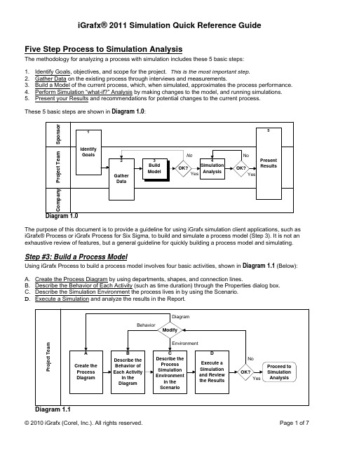
iGrafx® 2011 Simulation Quick Reference GuideFive Step Process to Simulation AnalysisThe methodology for analyzing a process with simulation includes these 5 basic steps:1. Identify Goals, objectives, and scope for the project. This is the most important step.2. Gather Data on the existing process through interviews and measurements.3. Build a Model of the current process, which, when simulated, approximates the process performance.4. Perform Simulation “what-if?” Analysis by making changes to the model, and running simulations.5. Present your Results and recommendations for potential changes to the current process.These 5 basic steps are shown in Diagram 1.0:The purpose of this document is to provide a guideline for using iGrafx simulation client applications, such as iGrafx® Process or iGrafx Process for Six Sigma, to build and simulate a process model (Step 3). It is not an exhaustive review of features, but a general guideline for quickly building a process model and simulating. Step #3: Build a Process ModelUsing iGrafx Process to build a process model involves four basic activities, shown in Diagram 1.1 (Below):A. Create the Process Diagram by using departments, shapes, and connection lines.B. Describe the Behavior of Each Activity (such as time duration) through the Properties dialog box.C. Describe the Simulation Environment the process lives in by using the Scenario.Execute a Simulation and analyze the results in the Report.D.A. Create a Process Diagram (Map or Flowchart)The Process diagram type supports all the features and functionality discussed in this guide. When the tool presents the Welcome dialog box, click the New Document button and choose Process.The Selector cursor: Click the left mouse button to select an object.Placement cursor: Click the left mouse button to place a shape/symbol.Departments:•Click the “Departments” icon in the Toolbox toolbar (the vertical toolbar on the left side of the window) •Choose Insert Department, which opens the Insert Department dialog box.•Enter a name for the department, and Click OK. You may also click the Apply button and add more departments.Add a Shape/Symbol:•Click on a Shape icon in the Toolbox toolbar.•Move the cursor into the process window. The cursor changes to the placement cursor (a pencil and shape). •Press, drag, and release the left mouse button to place the shape on the diagram.•Start typing to enter text. The text will be placed in the shape automatically.Connect Shapes/Symbols:•Move the Selector tool’s arrow cursor (or connector line tool’s line cursor) inside the source, or origin, shape.•Press and hold the left mouse button.•Drag the cursor to destination shape. The cursor automatically changes to the line cursor (pencil and line). •Position the cursor inside the destination shape, & release the mouse button; the line is automatically routed.Enter or Modify Text in a Shape, or on the Process Diagram:•Select the shape, if it isn’t already selected. Or click the “A” on the toolbox toolbar, and click in the diagram.•Type the text. Press the Esc (Escape) key when you are done typing.Display Shape/Activity Numbers:When a shape is placed on the diagram, a number is automatically assigned to the shape. By default the activity numbers are not displayed. To display activity numbers on the shapes:•Click on the Shape Numbering button in the Toolbox toolbar, and choose Show All Shape Numbers.To automatically renumber the shapes:•Click on the Shape Numbering button in the Toolbox toolbar, and choose Auto Renumber, then click OK. Please see the FlowCharter Quick Reference Guide for more information about diagramming with iGrafx.B. Describe the Behavior of Each Shape/ActivityMost shapes represent activities, and will contain behavioral information. As a general rule, during simulation a transaction enters the activity and visits each page of the Modeling category in the Properties dialog box starting with Inputs, and proceeding down through the Last Simulation page. The Process Guide (the Process page in the Guide category) allows quick entry of common data. Commonly used Modeling category pages are Inputs, Resources, Task, and Outputs.Display the Properties Dialog boxDouble-click the left mouse button on a shape, or click the right mouse button and choose Properties.Diagram 2.0: Inputs Diagram 2.1: Resources Diagram 2.2: Task Diagram 2.3: Outputs Inputs page: The Inputs page allows for the collection of transactions (see Diagram 2.0, above). The default is no collection. The most common forms of collection that are used in modeling:Batch: Collect multiple transactions in a basket and carry them through the process. The On Completion tab of the Task page contains a command to Unbatch the transactions, emptying the basket.Join: Merge multiple transactions together into a single transaction. Some data is merged, including attributes. Gate: Hold transactions at the gate until a condition is met and the gate is opened.Group:Transactions can enter an activity individually, and they are tagged with a group name.Introduce Transactions: Defines a point in the process where transactions are introduced. Choose None to specify that no transactions are generated here. Choose Using a Start Point to name the start point and then set up generators to introduce transactions into the activity. Choose Generate Here to specify that the simulator will generate a transaction when a condition occurs; such as an event happens, a period of time elapses.Resources page: The Resources page identifies the resources required to do work in the activity (see Diagram 2.1, above). iGrafx has a built-in resource named Worker. The Worker resource belongs to each department. When a department is added to the Process diagram, a worker is automatically created and allocated to the department. Creating other Labor or Equipment (non-worker) resources is done in the Scenario (see C. Describe the Process Environment in the Scenario).Many options may be specified for a resource; however, the following are the most important:•Choose the resource by type using the scroll down menu (The Default is Worker unless you change this). •Specify the count (number) of resources required to work on each transaction processed. The default is 1. •Specify how the resource is acquired. Usually the resource works for the activity, which is the default.To specify that more than one type of resource is required for an activity, click the Add button in the Resource page. To remove a specified resource from participating in an activity, choose the Delete button.Task page: The Task page defines the type of task the activity performs (see Diagram 2.2, above). The Step tab is used on most activities. The Task page defines the type of task, duration, special handling, etc.Types of Tasks: There are three types of tasks.Work: This task will use a resource to work on a transaction for the duration of the Task. Reported as Work. Process: This task is linked to a subprocess. During simulation, the transaction will move from this activity to a start activity on another diagram (subprocess). The transaction returns to this activity when it completes the subprocess. To create a subprocess:1. Choose Process from the drop-down menu for task type (subprocess is chosen automatically).2. Click on the New Process button.3. Enter a name for the process, and click OK.To view a subprocess, hold down the Shift key and double-click. You may also right-click and choosethe name of the subprocess to follow the link. The times in the subprocess will be collected in the report. Delay: This task blocks the transaction for the duration of the Task. Delay tasks do not usually use a resource. Duration: If the activity is Work or Delay, then task will have duration; default is zero (0). The duration may be:Constant: The same (constant) duration value for all transactions.Distributed: The duration value will range between a minimum and maximum value. The duration may be uniformly or normally distributed between the two numbers:•Uniform specifies every number between the two numbers has an equal probability of being used.•Normal specifies a normal (bell curve) distribution, which is centered between the two numbers. Expression: Equations may be defined to describe the duration of the activity. For details on building expressions, search the software Help system (Help menu) using keyword “duration expressions”.Value Class: Is an opportunity to classify the activity. The implied meanings are:VA: Value-Added. The customer is willing to pay us for this work; it adds value to the end product.NVA: No Value-Added. This work adds no value. Lean methodology refers to this as muda.BVA: Business Value-Added. This work is necessary for the business, but does not add value for the customer.Task Capacity, Schedule, and Overtime Behavior: Defines limits to the number of transactions processed and the processing timeframe. Also defines activity behavior with regard to the defined schedule.Limited Capacity:Limits the number of transactions that can be processed at one time.Limited Schedule:Specifies whether the task duration of the activity is limited to a schedule. Resourceschedules still apply for any resources required for the activity.Overtime Behavior:Specifies how the activity behaves if resources go out of schedule.On Completion: This tab of the Task page has functionality to complete transaction handling. Common choices: None: No special task ‘on completion’ behavior is defined. This is the default.Duplicate: Copies a transaction into multiple (count) identical transactions.Discard: Terminates the transaction. The transaction will not be counted in the simulation report. Unbatch: This undoes the “Batch” collection (see the Inputs page for information on Batch). Outputs page: The Outputs page describes how transactions leave the activity (see Diagram 2.3, above). A transaction will follow directed a connection line or lines to the Input of an activity. The Normal tab is used on most activities. The Normal tab defines how transactions follow lines, and Exceptions specifies any special outputs.Normal Tab: Specifies which of the lines the transaction will follow to an activity. The common choices are:All: This sends the transaction down all paths that leave the activity. This is the default. Ifthere is more than one path, an implicit duplication occurs, creating identical transactionsto be sent down each path.Decision: This sends the transaction into one of the paths specified, based on percentages orexpressions.Exceptions Tab: Define conditions where the activity terminates early, and the path to take. Common choices: None: This is the default choice; no special exception will occur.Timer:Sets a time limit on performing the activity; follow the exception path if the limit is reached.The Timer may be disabled at various points in the execution of the activity.Attributes page: Allows access to attributes, which are similar to programming variables and are used to communicate information and manage the flow of transactions through a process. For details on attributes, search the Help system using the keyword “attributes”.Last Simulation page: The Last Simulation page summarizes statistics for the activity from the last simulation.C. Describe the Process Environment in the ScenarioA Scenario describes the simulation environment for the process. A single file may contain multiple Scenarios.View the Scenario: You may view information in the Scenario “at a glance” in the Scenario window. To open the Scenario window, click the View Scenario button in the Modeling toolbar. Alternately, use the File menu and choose Components, and in the Components dialog, double-click the Scenario or right-click and choose View. The first four topics in the Scenario are the most important in getting started. Those topics are Run Setup, Generators, Resources, and the Schedules sub-topic under the Calendars topic.Diagram 4.0: Diagram 4.1:Run Setup GeneratorsDiagram 4.2: Diagram 4.3:Resources SchedulesRun Setup: The Run Setup topic sets simulation timing and how the results of simulation are placed in a report. Double-click on the Run Setup information in the Scenario to invoke the Run Setup Dialog (see Diagram 4.0, above). Of the many options you can specify, the most important are:Simulation Time tab:•Simulation Start: Specify when the simulation starts (default is a Weekday vs. by a specific Date). •Simulation End: The default is Transactions Complete. Most often you’ll want to specify a specific duration for simulation (Custom). To specify a custom end for simulation:o Choose Custom from the Simulation End scroll down menu.o Choose a duration time unit (Hours, Days, Months, etc.)o Enter a duration (simulation end) value.Initialization/Reports tab: Specify how the simulation results are to be saved to the report (default is Create).Generators: During simulation, generators introduce transactions into the process. Of the many options you can specify, the most important is Generator Type. The generator type determines other data to specify. Common types of Generators are:Completion: The Completion generator introduces transaction(s) into the process when the previous transaction(s) has completed processing. It will place one transaction at a time, or a group of transactions, in theprocess until it (they) reaches the Maximum count. The default is a Max count of 1.Demand: The Demand generator introduces a transaction whenever the named resource (for example, Worker) is available, in the department that has the Start activity for this generator.Interarrival: The Interarrival generator specifies the duration of time between transactions arriving in the process.There are many options; you may want to start with a simple Constant or Distributed interarrival time.•Constant: The same (constant) time between transactions entering the process.•Distributed: The time between transactions entering the process will range between two values.•Expression: The expression can use math functions, such as ExponDist() for exponential arrivals. Timetable: The Timetable generator introduces transactions at specified intervals, over a span of time. The table may be repeated. To modify the timetable generator, click the Modify Timetable button, and a barchart appears. The X-axis shows the time intervals and the overall time span, and the Y-axis showsthe number of transactions introduced during each interval. The values of interest are:•Total Span. The total span of time covered by the timetable pattern given. For example, 1d (1day) indicates that every day the given pattern should repeat.•Time Resolution. The smallest interval of time in the bar chart.Resources: The Resource topic is where resources used by the process are created, modified, and managed.Double-click the left mouse button on the Resources topic/data in the Scenario to obtain the Resources dialog box(see Diagram 4.2, above).To add a resource, click the Add button, which adds a new type of resource (other than Worker).•Enter a name under Resource Name. You cannot use spaces in the name.•Choose a Resource Classification; we recommend Labor or Equipment, as Other has limited use.To modify a resource, select the resource in Existing Resources list.•Resource Count: Enter the number of that resource available to the process.•Schedule: Choose the schedule that indicates when the resources are available and inactive (see below).•Resource Cost: Specify the hourly pay rate, and/or hourly rate in overtime, for the resource.Schedules: Schedules are spans of time. The time will be either active or inactive. You can use any ofseveral built-in schedules (see Diagram 4.3, above). The default schedule is the Standard schedule, which isMonday through Friday, 8 AM to 5 PM, with 1 inactive hour for lunch. For details on creating and modifyingschedules, search the software Help system using the keyword “schedules”.D. Execute Simulation and Analyze Results in the Reportor Run a Simulation: To run a simulation,from the Model menu, choose Run and then Start. You can“trace” simulation by first entering Trace mode, and then running simulation. The Control menu’s Trace Colorscommand shows the colors’ meanings. When simulation is complete, a Report is presented for review.Report Structure: The first four of the Report tabs contain sets of commonly used statistics captured duringsimulation: Time, Cost, Resource, and Queue (Waiting in Line) information. The fifth tab, Custom, is blank; youmay add a report element (table or graph) to the Custom tab by copying and pasting an existing report element, orcreating a new report element from the Report menu.Report Results: Basic statistics are gathered about process times, costs, resources, and waiting lines or queues.You may also create your own custom statistics. The basic statistics are categorized depending on whether theyapply to transactions, resources, or activities (see Table 5.0, below).Transaction Resource ActivityProcess Performance From the Transaction’s Perspective Process Performance From theResource’s PerspectiveDetailed Information About WhatOccurred At Each ActivityCompletion Count Number of Workers (Count) Cycle Time (Avg.)Cycle Time (Avg.) Utilization (Util. %) Work Time (Avg.)Work Time (Avg.) Busy Time (Avg.) Wait Time (Avg.)Wait Time (Avg.) Idle Time (Avg.) Costs (VA, NVA, BVA) Resource Wait Time (Avg.) Out Of Service Time (OOS) # Trans. Wait (Tavg, Tot., Max) Blocked Time (Avg.) Inactive Time (Avg.) # Trans. at Activity (Tavg, Max) Inactive Time (Avg.) Overtime (OT) # TransactionsService Time (Avg.) Costs (Tot., Std., OT, Busy)Costs (VA, NVA, Labor, Equip.)Table 5.0 Some Common Default Report StatisticsNote that placing your cursor over a statistic heading in the report will produce a yellow tooltip that explains the statistic in more detail. The tooltip will not, however, explain summarizations like Min, Max, Average, Total, etc. Basic Transaction & Activity Time Statistics: The 4 basic time statistics are:•Work Time:The time accumulated doing work (Task page Duration).•Resource Wait Time:The time accumulated waiting to obtain a resource (Resources page).•Blocked Time:The time accumulated waiting in collection (Inputs page) and in delay (Task page). •Inactive Time: The time accumulated waiting for a resource that is inactive or out of schedule. Composite Transaction & Activity Time Statistics: The 4 statistics constructed from the basic statistics are: •Cycle Time:Blocked Time + Resource Wait Time + Inactive Time + Work Time•Service Time:Blocked Time + Resource Wait Time + Work Time•Wait Time:Blocked Time + Resource Wait Time + Inactive Time•Service Wait Time:Blocked Time + Resource Wait TimeBasic Resource Time Statistics: The 4 basic resource time statistics are:•Busy Time:The time the resource is acquired; e.g. active & working (Task page Duration). Paid. •Idle Time:The time the resource is active & in schedule, but not busy. Also paid time.•Out Of Service (OOS): The time the resource is scheduled to be active & also unavailable. Paid or unpaid. •Inactive Time:The remaining time when the resource is not scheduled to be available or OOS. Add a New Report Element:•From the Report menu, choose Add Element.•Follow the Wizard to Define the Statistic category, Structure, Filtering, and Format of the Report Element. Turn a Tabular Report Element Into a Graph:•Double-click on the Report Element to obtain the Edit Report Element dialog box.•Choose the Format tab.•From the “Display As” scroll down menu, choose Graph.•Choose the style of graph you wish to display; for example, a 2D bar chart.• Click OK.Time-Weighted Average Resource UtilizationWorker As-Is70.24Hire a Worker35.12Name a Simulation Run:1. From the Report menu, choose Simulation Data.2. Double-click the simulation run you want to name.3. Type in the new name and click OK.Copying (Exporting) Report Data to Other Applications:1. Click on the report element to select it. You may select more than one element by using your shift key.2. Press Ctrl+C to copy, right-click and choose copy. Make the other application active, and paste withCtrl+V; or from the Edit menu, choose Paste, or Paste Special if available.For more information on iGrafx Training and Consulting services, please use the following contact information: Email:info@ Phone: 503-404-6050 Fax: 503-691-2451Mail:7585 SW Mohawk Street; Tualatin, Oregon 97062。
Matlab第五章 Simulink模拟电路仿真
第五章Simulink模拟电路仿真武汉大学物理科学与技术学院微电子系常胜§5.1 电路仿真概要5.1.1 MATLAB仿真V.S. Simulink仿真利用MATLAB编写M文件和利用Simulink搭建仿真模型均可实现对电路的仿真,在实现电路仿真的过程中和仿真结果输出中,它们分别具有各自的优缺点。
武汉大学物理科学与技术学院微电子系常胜ex5_1.mclear;V=40;R=5;Ra=25;Rb=100;Rc=125;Rd=40;Re=37.5;R1=(Rb*Rc)/(Ra+Rb+Rc);R2=(Rc*Ra)/(Ra+Rb+Rc);R3=(Ra*Rb)/(Ra+Rb+Rc);Req=R+R1+1/(1/(R2+Re)+1/(R3+Rd));I=V/Req武汉大学物理科学与技术学院微电子系常胜ex5_1武汉大学物理科学与技术学院微电子系常胜武汉大学物理科学与技术学院微电子系常胜注意Simulink仿真中imeasurement模块/vmeasurement模块和Display模块/Scope模块的联合使用Series RLC Branch模块中R、C、L的确定方式R:Resistance设置为真实值Capacitance设置为inf(无穷大)Inductance设置为0C:Resistance设置为0 Capacitance设置为真实值Inductance设置为0L:Resistance设置为0Capacitance设置为inf Inductance设置为真实值武汉大学物理科学与技术学院微电子系常胜MATLAB方式:步骤:建立等效模型→模型数学化→编写M文件计算→得到运算结果优点:理论性强,易于构建算法、模型缺点:较复杂,对电路观测量更改时需更改M文件适用范围:大系统抽象和原理性建模Simulink方式:步骤:选取模块→组成电路→运行仿真→观测仿真结果 优点:直观性强,易于与实际电路对应,易于观察结果 缺点:理论性不强,对电路原理不能得到解析适用范围:具体电路仿真武汉大学物理科学与技术学院微电子系常胜5.1.2 Power System Blockset模块集及powerlib窗口Power System Blockset模块集是MATLAB中专用的电路仿真模块集,其中内含有Electrical Source、Elements等子模块库,而电路仿真常用的DC Voltage Source、Series RLC Branch、Current Measurement等模块都被包含在这个模块集中。
MODTRANTP5文件参数设置说明
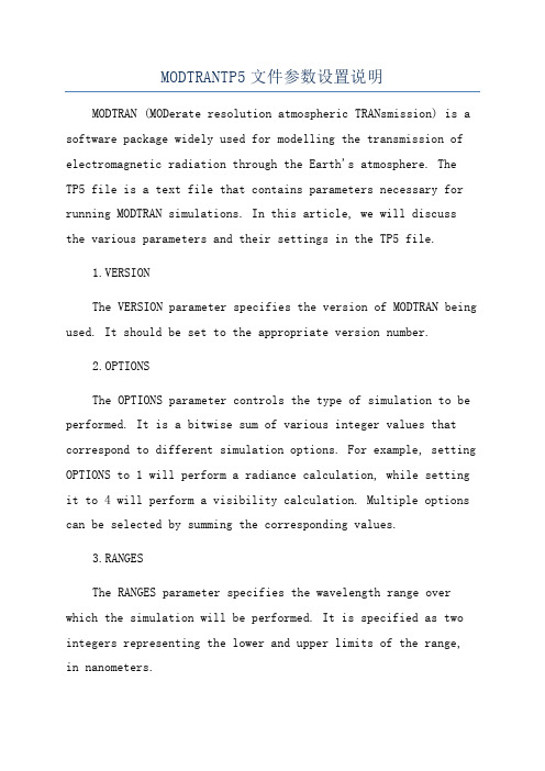
MODTRANTP5文件参数设置说明MODTRAN (MODerate resolution atmospheric TRANsmission) is a software package widely used for modelling the transmission of electromagnetic radiation through the Earth's atmosphere. TheTP5 file is a text file that contains parameters necessary for running MODTRAN simulations. In this article, we will discuss the various parameters and their settings in the TP5 file.1.VERSIONThe VERSION parameter specifies the version of MODTRAN being used. It should be set to the appropriate version number.2.OPTIONSThe OPTIONS parameter controls the type of simulation to be performed. It is a bitwise sum of various integer values that correspond to different simulation options. For example, setting OPTIONS to 1 will perform a radiance calculation, while setting it to 4 will perform a visibility calculation. Multiple options can be selected by summing the corresponding values.3.RANGESThe RANGES parameter specifies the wavelength range over which the simulation will be performed. It is specified as two integers representing the lower and upper limits of the range,in nanometers.4.REFRACTIVITYThe REFR activity parameter controls the modeling of refractivity in the atmosphere. It can be set to either 0 (no refraction), 1 (ignore dispersion), or 2 (include dispersion).5.WATER6.OZONEThe OZONE parameter specifies the total columnar amount of ozone in the atmosphere, in Dobson Units (DU). It affects the calculation of transmittance in the ultraviolet region.7.AEROSOLSThe AEROSOLS parameter controls the modeling of aerosols in the atmosphere. It can be set to either 0 (no aerosols), 1 (urban aerosols), or 2 (continental aerosols).8.ALTITUDESThe ALTITUDES parameter specifies the altitude levels at which calculations will be performed. It is specified as a list of integers representing the altitude levels, in kilometers.9.SOLARThe SOLAR parameter specifies the solar spectrum to be used in the simulation. It can be set to either 0 (extraterrestrial spectrum), 1 (solar constant), or 2 (constant solar spectral irradiance).10.GROUNDThe GROUND parameter specifies the type of ground surface to be simulated. It can be set to either 0 (flat surface), 1 (Lambertian surface), or 2 (user-defined BRDF).11.VIEWINGThe VIEWING parameter specifies the atmospheric pathway for the observer. It can be set to either 0 (vertical path), 1 (slant path), or 2 (user-defined).12.ANGLESThe ANGLES parameter specifies the viewing and solar angles to be used in the simulation. It is specified as a list of integers representing the azimuth and zenith angles of the observer and the sun, respectively.These are some of the key parameters and their settings in the MODTRAN TP5 file. Other parameters like aerosol models,solar zenith angles, and atmospheric profiles can also be modified as per the requirements of the simulation. Understanding and configuring these parameters accurately is crucial for obtaining accurate and meaningful results from the MODTRAN simulations.。
[电路与模拟电子电路PSpice仿真分析及设计 (5)[67页]
![[电路与模拟电子电路PSpice仿真分析及设计 (5)[67页]](https://img.taocdn.com/s3/m/3481919a2cc58bd63086bd4d.png)
图4-2 新建工程窗口
4.1.1 基尔霍夫定律应用与仿真分析
• 单击OK按钮,新工程建立后, 软件将自动打开空白的绘图窗 口。选择Place→Part功能菜单选 取 元 器 件 , 如 图 4-3 所 示 。 在 “Part:”栏输入所需元器件的名 称,或者在元器件下拉列表中
直接选取元器件,元器件的外
0.8us
1.0us
4.1.2 叠加定理应用与仿真分析
• 将上述仿真结果叠加可得,I(R2)=1+(-0.5)=0.5A, U(I1)=5+2.5=7.5V,验证了叠加定理的正确性。
4.1.3 戴维南定理仿真分析
• 【例4-3】 在窗口显示 的空白绘图区中,通 过添加元器件和连线 操作,实现图4-19所示 的电路图,求流过电 阻R的电流I,并验证戴 维南定理。
过添加元器件和连线 操作,实现图4-1所示 的电路图,分别用支
路电流法与节点电压
法求流过各支路的电
流,并通过仿真验证 。
图4-1 原始电路图
4.1.1 基尔霍夫定律应用与仿真分析
• 1.绘制电路图
• 首先打开Capture程序 ,在编辑窗口中选择 File→New功能菜单或 者单击按钮,出现新 建工程窗口,新建一 个空白工程文件,如 图4-2所示。
图4-19 原始电路图
第四章
电路基础仿真分析
杨维明,谌雨章
4.1 电路基本定理仿真分析
• 4.1.1 基尔霍夫定律应用与仿真分析 • 4.1.2 叠加定理应用与仿真分析 • 4.1.3 戴维南定理仿真分析 • 4.1.4 诺顿定理仿真分析
4.1.1 基尔霍夫定律应用与仿真分析
• 【例4-1】 在窗口显示 的空白绘图区中,通
VIBRO_5_Porous_materials-ACTRAN多孔材料模型介绍

Theory Poro-elastic Materials ACTRAN Training –VIBROPoro-elastic material in a carUsed for discretizing porous media, i.e.the fluid and solid phases in oneelement.Based on Biot Model: skeleton, fluid,solid/fluid interactionu-p formulation : u (solid displacement)and p (fluid pressure within the pores)Picture courtesy of Rieter AutomotivePorous materials are used by different porous models (rigid, UP, lumped, Delany-Bazley)Material properties are divided in: Fluid properties BEGIN MATERIAL IdPOROUSFLUID_DENSITY valueFLUID_BULK_MODULUS value VISCOSITY valueFluid-skeleton propertiesMicromodel parametersElastic parametersAll values can be complexTHERMAL_CONDUCTIVITY value CP valueCV valuePOROSITY valueFLOW_RESISTIVITY valueBIOT_FACTOR value TORTUOSITY valueVISCOUS_LENGTH value THERMAL_LENGTH value SOLID_DENSITY valueYOUNG_MODULUS value POISSON_RATIO valueEND MATERIAL IdSyntax in the ACTRAN input file:Definition in ACTRAN/VI:BEGIN MATERIAL Id POROUSFLUID_DENSITY valueFLUID_BULK_MODULUS value POROSITY valueFLOW_RESISTIVITY value BIOT_FACTOR value Fluid propertiesFluid-skeletonTORTUOSITY value VISCOSITY valueTHERMAL_CONDUCTIVITY value CP value CV valueVISCOUS_LENGTH value THERMAL_LENGTH value SOLID_DENSITY value YOUNG_MODULUS value POISSON_RATIO value END MATERIAL IdpropertiesMicromodel parametersElastic parametersThe RIGID_POROUS component is used fordiscretizing a porous medium when the material skeleton can be assumed as rigid.Points to a valid acoustic POROUS materialSupported topologies(no elastic properties needed)Unknowns: fluid pressure (1 dof/node)(skeleton displacement is assumed rigid, hence u=0)Based on a reduced Biot’s modelSyntax in the ACTRAN input file: Definition in ACTRAN/VI:BEGIN COMPONENT IdRIGID_POROUSMATERIAL valuePOWER_EVALUATION valueEND COMPONENT IdPorous Material Properties required:FLUID_DENSITYFLUID_BULK_MODULUSPOROSITYFLOW_RESISTIVITYBIOT_FACTORTORTUOSITYVISCOSITYTHERMAL_CONDUCTIVITY[VISCOUS_LENGTH][THERMAL_LENGTH]The LUMPED_POROUS component is usedfor discretizing porous medium when the material skeleton can be assumed as extremely soft (E=0)Supported topologiesPoints to a valid acoustic POROUS material(solid density is needed for inertia)Unknowns: fluid pressure (1 dof/node)(skeleton displacement is assumed soft, hence u=w)Based on a reduced Biot’s modelSyntax in the ACTRAN input file:Porous Material Properties required:Definition in ACTRAN/VI:BEGIN COMPONENT Id LUMPED_POROUS MATERIAL valuePOWER_EVALUATION value END COMPONENT IdFLUID_DENSITYFLUID_BULK_MODULUS POROSITYFLOW_RESISTIVITY BIOT_FACTOR TORTUOSITY VISCOSITYTHERMAL_CONDUCTIVITY [VISCOUS_LENGTH] [THERMAL_LENGTH]SOLID_DENSITYPorous UP Component (1)Related to porous material with an elastic skeleton while the rigid and lumpedformulations assume a perfectly rigid or a perfectly soft skeleton respectivelyPoints to a valid acoustic porous material (elastic properties needed)BEGIN COMPONENT Id POROUS_UPMATERIAL value POWER_EVALUATION value END COMPONENT IdSupportedUnknowns: fluid pressure and soliddisplacement(4 dof/node)Based on the Biot modeltopologiesDefinition in ACTRAN/VI:Porous UP Component (2)Syntax in the ACTRAN input file:Porous Material Properties required:BEGIN COMPONENT Id POROUS_UPMATERIAL valuePOWER_EVALUATION value END COMPONENT IdFLUID_DENSITYFLUID_BULK_MODULUS POROSITYFLOW_RESISTIVITY BIOT_FACTOR TORTUOSITY VISCOSITYTHERMAL_CONDUCTIVITY [VISCOUS_LENGTH] [THERMAL_LENGTH] SOLID_DENSITY YOUNG_MODULUSProperties involved in porous elementsList of the poro-elastic materials propertiesThe following properties are measured using an experimental set-up described in the following slides:Young modulus and loss factor of the foam skeleton >Porosity >Weight of the foam and in particular of the material constituting the foam > Flow resistivity >Tortuosity >Fluid bulk modulusThe bulk modulus Q measures the compressibility of the foam. It is therefore an average of the fluid and skeleton bulk moduli, or, if simplified, the compressibility of the fluid within the pores :fs f K K K Q 1111≈+=Young modulus E and loss factor of the foam skeleton Characterize the stiffness and damping of the porousskeletonThe transfer function between the displacement at the topand bottom of the sample give the Young and loss modules from which the loss factor can be foundDynamic ModulusPicture courtesy of Walter Lauriks auriks -KU LeuvenBack to the list >Porosity ΩPorosity is the percent open area within the material -it allows the sound waves to propagate into the materialFor a sample of total volume Vt of a porous material contains a volume Vf of fluid and Vs of solid. The porosity is defined as:Ω==V V V VVf fs +=−V V1Picture courtesy of Walter Lauriks -KU LeuvenSolid densityThe solid density to enter is the density of the material of the skeleton (not the density of the porous material). It can be related to the porous material density by:Weight of foam = weight of fluid phase + weight of solid phases s f f t p V V V ρρρ+=ff V V ρρStatic Resistivity RThe fluid flowing through a porous material encounters a resistance related to the viscous interaction forces between the fluid and the solid skeleton.Flow resistance is the result of porosity, tortuosity and cell structure of a material and is often a good measure of how absorptive a material will beSet-up: a pressure difference is imposed between the two sides of a sample (thickness=h) and the global air flux v is measured.Static resistivity: the flux is constant and not oscillatingPicture courtesy of Walter Lauriks -KU LeuvenBack to the list >Tortuosity α∝Tortuosity is the property thatprevents direct flow through thematerialIt measures the complexity of the pathan air particle must follow to proceedfrom one point to another point.Tortuosity α∝Two measurement techniques:the ultrasonic technique: a thin sample is placed between an ultrasound source (A) and a receiver (B). The propagation speed with and without thesample characterizes the tortuosity.the electrical technique: the test cell is filled by a conducting electrolyte and the conductivity of fluid alone is compared to the conductivity in presence ofa saturated samplePicture courtesy of Walter Lauriks -KU LeuvenBack to the list >Tortuosity α∝21Copyright Free Field TechnologiesBiot Parameter αThe Biot factor α is a coupling coefficient and is equal to 1 for most materials. Its origin has to be found in soil mechanics, for which the Biot theory has been developed The set of foam parameters can be validated by doing an impedance test (simulation/measurement comparison). A sample of the foam material is placed in a Kundt tubePicture courtesy of Walter Lauriks - KU LeuvenBack to the list >22Copyright Free Field TechnologiesMicro-Models (Allard and Johnson)Expression for R and Q as functions of frequency can be obtained (model of Allard and Johnson)λTwo parameters play an important role:Λv characteristic viscous length Λt characteristic thermal lengthBack to the list >23Copyright Free Field TechnologiesViscous and thermal lengthsParameters driving the micro-model Measured using the tortuosity experimental set-up. Two measurements: one with air the other with helium24Copyright Free Field TechnologiesImpedance tubeA foam sample of 2.9 cm is placed at the end of an impedance tube. The full list of foam properties is given (see table) The absorption coefficient is measured and compared to Actran as well as an analytical solution25Copyright Free Field TechnologiesPhysical behavior – ApplicationsCopyright Free Field TechnologiesInsulation, absorption, transmissionObjective of the trim:To improve the acoustic insulation of a specific component (transmission loss) To damp the structural vibrations To optimize the acoustic absorption of the vehicle compartmentAirborne transmission: Insulation / AttenuationStructure-borne transmission: DampingInternal sources: AbsorptionTrimmed component:Picture courtesy of Rieter AutomotiveCarpets: roof, floor, dash panels… Glass set: windshield, side windows,…27Copyright Free Field TechnologiesDamping of cavity modes using acoustic treatmentMeasurement2Effet amortissant des matériaux absorbants, Barrelet S., Zhang C., Diallo A. – Renault; Mahieux B. – Teuchos E., SIA 2002, Le Mans, France28Copyright Free Field TechnologiesDamping of cavity modes using acoustic treatmentMeasurement Actran simulations29Copyright Free Field TechnologiesMulti-layer composite: analysisFrame Heavy LayerPicture courtesy of Rieter AutomotivePorous Layer Damping Layer Metal LayerPicture courtesy of Rieter Automotive30Copyright Free Field TechnologiesDecoupled system: vibration insulationThe multi-layer acts as a double mass-spring system where the mass is made of the sheet metal and heavy layer and the spring stiffness isdetermined by the skeleton stiffness, the resistivity of the porousmaterial and the compressibility of the air inside the pores10Amplification ReductionBelow the cut-offRadiation efficiencyThenoise radiation by the panel without treatment is much higher than this ofthe treated panel becauseof:the lower radiation efficiency of the heavy septumlayer due to the shorterwavelength of bending wavesthe reduced vibrationlevel, the increased vibration damping (see next slides)steelDamping in the heavy layerBending wave celerity in the top and bottom layer are much different …… and damping in the heavy layer and the porous material further reduces the vibration amplitudes on the treated side.septumsteelDamping in the porous layer: flowresistancePicture courtesy of Rieter AutomotiveThe relative velocity between the fluid and the skeleton is responsible for intense resistive dissipation in the porous layer (flow resistance R)The relative acceleration also causes dissipation through the tortuosity termRTC-III (from French, Rayonnement des Tôles de Carrosserie)simplified representation of a floor panel of a passenger car body measure of the efficiency of damping materials and treatments The system comprises essentially three parts:•An upper cabin which servesas a reception chamber.•The excitation part: a verystiff frame excited by a shaker,•The lower cabin, on which the excitation assembly is placedREMARK:While testing: The boxis in contact with thepanelAfter the test: the boxis lifted to change thematerial treatmentTôle nue en vibratoire-20-10102030405050100150200250300350400450T r a n s m i s s i b i l i t é (/)Mesure tole nue Simulation ACTRANStructural response: steel, foam, septumMesures vs. ActranTrimmed panelMesures vs. ActranSteel onlyAcoustic response in the cavity: steel + foam + septumMesures vs. Actran Trimmed panel Mesures vs. Actran Steel only。
SolidWorks Simulation图解应用教程(五)
SolidWorks Simulation图解应用教程(五)
陈爱华; 方显明
【期刊名称】《《CAD/CAM与制造业信息化》》
【年(卷),期】2009(000)011
【摘要】一、横梁的力学分析在实际工程设计中,各种机器设备和工程结构都是由若干个构件组成的。
这些构件在工作中都要受到各种力的作用,应用静力学的知识,我们可以分析计算这些构件所受到的外力情况。
为保证机器设备和工程结构在外力作用下能安全可靠地工作,就必须要求组成它的每个构件均具有足够的承受载荷的能力。
【总页数】4页(P101-104)
【作者】陈爱华; 方显明
【作者单位】浙江金华技师学院
【正文语种】中文
【相关文献】
1.SolidWorks Simulation图解应用教程(七) [J], 方显明
2.SolidWorks Simulation图解应用教程(二) [J], 方显明
3.SolidWorks Simulation图解应用教程(三) [J], 方显明
4.SolidWorks Simulation图解应用教程(一) [J], 方显明
5.SolidWorks Simulation图解应用教程(六) [J], 陈爱华;方显明
因版权原因,仅展示原文概要,查看原文内容请购买。
- 1、下载文档前请自行甄别文档内容的完整性,平台不提供额外的编辑、内容补充、找答案等附加服务。
- 2、"仅部分预览"的文档,不可在线预览部分如存在完整性等问题,可反馈申请退款(可完整预览的文档不适用该条件!)。
- 3、如文档侵犯您的权益,请联系客服反馈,我们会尽快为您处理(人工客服工作时间:9:00-18:30)。
2102008,20(2):210-215A MULTI-BODY SPACE-COUPLED MOTION SIMULATION FOR A DEEP-SEA TETHERED REMOTELY OPERATED VEHICLE *ZHU Ke-qiang, ZHU Hai-yang, ZHANG Yu-song, GAO JieMaritime College, Ningbo University, Ningbo 315211, China, E-mail: zhukeqiang@ MIAO Guo-pingSchool of Naval Architecture, Ocean and Civil Engineering, Shanghai Jiaotong University, Shanghai 200030, China(Received May 8, 2006, Revised February 28, 2008)Abstract: A multi-body coupled dynamic model is developed to simulate the motion of a Tethered Remotely Operated Vehicle (TROV) system. A strong nonlinear coupling motion between umbilical tether and ROV is discussed .The movement of ROV is considered as six-degrees of freedom. The lumped mass model is applied and an averaged tangential vector technique is included in the three-dimensional dynamic response equations of the cable-segments. The model can simulate the three-dimensional transient coupled motion of the complex multi-body system in typical ship maneuvering conditions and can be used in either a towing problem or a tethered underwater vehicle problem. Simulation results are seen to fit well with the experiment. Key words: cables, ROV, hydrodynamics, coupled motion1. IntroductionDynamic analysis of marine cables has been of interest owing to their wide applications in ocean engineering [1-5]. Experimental study will be the most reliable method to predict the dynamic behavior of marine cable systems. Grosenbaugh [6] measured the motion and tension of a deeply moored buoy. Yoerger et al.[7] and Hover et al.[8] measured the motion of a deeply towed underwater vehicle system.However, the experimental study is time consuming and costly. There exist also some limitations and difficulties in the experiment [9, 10]. The depth limitations of the existing basin laboratories pose questions to the validity of the testing depth. Small scales introduce uncertainties related to viscous effects owing to the nature of the scaling laws. In system design, coupled*Project supported by the National Natural Science Foundation of China (Grant Nos. 10572063 and 50639020), the State Key Laboratory of Ocean Engineering (Shanghai Jiaotong University) (Grant No. 0502) and the Program for Changjiang Scholars and Innovative Research Team in University ( Grant No. IRT0734).Biography : Zhu Ke-qian g (1956-) , Male, Ph. D., Professornumerical analysis will still be an important and practical tool in combination with model tests.Two kinds of modeling techniques are available to predict the response of tethered systems: the continuous (closed-form, analytical) and the discrete models. Continuous models can provide quick estimates of several dynamic characteristics of tethered systems, including motion and tension spectra, transfer functions, the natural frequencies, and the onset of slack in the tether. Both Niedzwecki et al.[11]and Huang et al.[12] used a model of single-degree freedom to characterize the response of a vertically suspended system subject to sinusoidal forces. These simple models provide a first-order approximation to a vertically tethered system. Niedzwecki and Thampi [13]also derived a set of closed equations that represent a multi-segment drill string. Continuous models are effective tools but they also have several limitations. For example, equivalent linearization techniques have to be used to approximate the quadratic drag [14, 8], and the coupled motion equations of ROV are rarely included in these models. Moreover, these analytical models are invalid for a slack tether, which is the precursor of snap-loads.211Discrete models are not constrained by these limitations. They are valid for several non-linear properties like quadratic drag and spatially varying properties of cables. Various components such as ROV cages or in-line clumps can be easily added to the models. Niedzwecki and Thampi [11] developed a multi-segment lumped-parameter model of a drill string connecting a ship to a sub-sea package and used it to investigate snap load. Driscoll and Biggins [15]performed a preliminary study of a strictly vertical caged ROV system using a similar discrete method.The article presents a general multi-body model of space coupled motion for a deep-sea Tethered Remotely Operated Vehicle (TROV) system. A strong nonlinear coupling motion principle between the umbilical tether and the vehicle is discussed.The movement of ROV is considered as six-degrees of freedom. The lumped mass model is applied and an average tangential vector technique is included in the three dimensional equations of the cable-segment. Snap loads that can damage the armour and internal conductors of the tether can be predicted by computing the dynamic tension and the instant configuration. The investigation has an important meaning in avoiding resonance, surviving in resonance, extending the cable life, broadening the operational area of the ROV, or insuring docking and calling-back ROV safely, as well as saving the trial expense.2. Six-degrees freedom motion equations of TROV 2.1 Coordinate systemsTwo orthogonal coordinate systems are used to establish the present dynamic model. One is a global coordinate system ˄,,,E [K ]˅fixed at the ocean surface ship with origin at E ,]axis pointing vertically down to the water, and the K [, axes being in two mutually perpendicular horizontal directions. The other is a local coordinate system (o ,x , y , z ) fixed on the vehicle with origin at o ,x axis pointing to the nose of the vehicle, z axis pointing to the belly of the vehicle, and the y axis completing the right-hand system with the other two axes. The transformation of forces and motions from global to the local coordinate system can be fulfilled by the transformation matrix [T B ].»111213212223313233[]=B T T T T T T T T T T ªº«» ««» ¬¼(1)where11=cos cos T T \,12=cos sin T T \ˈ13=sin T T ˈ21=sin sin cos cos sin T M T \M \ ˈ22=sin sin sin cos cos T M T \M \ ˈ23=sin cos T M T ,31=cos sin cos sin sin T M T \M \ ˈ32=cos sin sin sin cos T M T \M \ ˈ33=cos cos T M Tand ,,\T \ are the Euler angles. The orientation of the vehicle in global coordinates can be specified bythe vector Eo r fromE to o .2.2 Inertia force on ROVSince all vehicles have a longitudinal symmetric plane xoz (), the added mass coefficients A =0G y ij with (I +j ) odd are all zeros. The mass matrix [M ]consisting of all the coefficients of inertia and added mass terms is defined as11223342445153556266000symmetric[]=000000m m m M m m m m m m m ªº«»«»«»«»«»«»«»«»¬¼(2)where1111=+m m A ˈˈ2222=+m m A 3333=+m m A ˈˈ4444=+xx m I A 5555=+yy m I A ˈˈ6666=+zz m I A 5115=+G m mz A ˈˈ4224=+G m mz A 6226=+G m mx A ˈ5335=+G m mz A212The remaining added inertial terms are^`^`T12345661=I I I I I I I F F F F F F F u where221[(+)+I G ]+G F m qw vr x q r z pr 632=1(jj j qArA V ¦)Rj +G )Rj ]+G (3a)2()I G F m ru wp z qr x pq(3b)613=1(jj j qApA V ¦223[(+)+I G F m pv uq z q r x pr621=1()jj Rj j pArA V ¦ 3(c)4()+[()I zz yy G F I I qr m z pw ru ]++) 22()+yx xx yx r q J J qp J pr66532=1(++jj Ry j Rz j R j qArA V A V A V ¦j (3d)5I F =()+[()xx zz G G I I rp m z qw rv x <+G 22()]+()zx xy qw rv p r J J rq 6461=1+(++xy jj Rz j j J qp rApA V A ¦ (3e)3)Rx j Rj V A V 6()+[I yy xx F I I pq m x <22()]+()xy yz ru pw p q J J pr +6542=1+(++xx jj Rx j j J rq qArA V A ¦1)Ry j Rj V A V (3f)where V Rj is the velocity of the vehicle relative to the fluid, and u,v,w,p,q,r are the motion parameters of ROV in the local coordinate system. 2.3 Weight, buoyancy and thruster forcesThe gravitational force and buoyant force are defined in the global coordinate system, and therefore, they must be transformed to the local coordinate systems:+=()G B B m g U <F F ^`Tsin cos sin cos cos TT MT M (4)(+)=(G G B B G B B g mz z )U u u <R F R F ^ (5)`T Tcos sin sin 0T MTThese forces can be combined into a dynamic vector {F CB }.The resultant force and moment of N thrusters can be expressed as=1=i Nr i ¦F F (6)=1=1=+i i N Nr T T i i u ¦¦M M R F (7)The magnitudes of thrust and moment owing to the i th thruster are2=i i T T i 4i F K n D U < (8) 2=i i T Q i 5i M K n D U < (9)where D i is the diameter of the i th thruster, n i is the rotate speed of the thruster shaft, and K Ti , K Qi are the coefficients of the thrust and the torque, respectively, expressed as functions of the advanced coefficient J=V n /(nD ). These two forces are then combined into a dynamic vector {F T }.2.4 Non -inertia hydrodynamic forcesAll the non-inertia hydrodynamic forces can be expressed as:^`,,223,,=2x y z F RR X Y ZF V F C U(10a)213^`,,523,,=22x y z F R R N K M N F V C R UU<^`T,,,,p q r N N N p p q q r r C < (10b)where(,)Fx C D E ,(,)Fy C E J ,(,)Fz C D J , , , Np C Nq C Nr C are six hydrodynamic coefficients of ROV and1=tan ()RzRxV V D (11a) 1=tan ()Ry RxV V E (11b)1=tan (RzRyV V J (11c) Hydrodynamic coefficients owing to the speed of transport motion such as drag coefficient, moment coefficient etc. can be obtained by model tests. The hydrodynamic coefficients owing to the accelerations and angular accelerations of the vehicle can be obtained by means of Planar Motion Mechanism. All these forces are then combined into a dynamics vector ̗F F ̙.2.5 Umbilical cable forceThe umbilical cable force is one of the most important nonlinear disturbance force on ROV when the current is strong and the cable length is long enough. The movement of a flexible cable moving in fluid can be described by the following lumped parameter equation [4]:212[]d ()=++d i i i i i i t tO r W D T T (12) where []i O is the cable mass per unit length, is the position vector of the i th lumped mass with respect to the fixed inertial reference, and is the gravitational force of i th lumped mass.i r i W The drag force lumped onto the i th node can be expressed as follows:11=(+)(+4i i i i i ti Rti Rti l d l d C SD U U )ni Rni Rni C U U where i ,C t C ni are the tangential and normal drag coefficients of the cable in the i th link, respectively,and Rti U ,Rni Uare the tangential and normal components of the relative speed at the i th node.d =[()]d iRti c i i t<r U U W W (13a) d =d iRni Rti tr U U 1) (13b) The unit tangential vector [4] at the i th node is defined as21=(=i i r r W (14a)1+1+11=(=2i i i i i i N ,1)r r r r W (14b)1=(=i N N i N ) r r W (14c)The tension force exerted in the i th link can be calculated by the position of the nodes+12+1=(14i ii i i i id E l S)ir r T r r (15) The cable force on ROV can be obtained by the transformation matrix [T B ] as>@^T=c B N c c c T X Y Z {F T ` (16a) ^`T=c c cz ccx c cz ccx c R Y R Z R X R Y u R F (16b)where ^`T=c cxcycz R R R R is the position vector oftethered point at the body coordinate system of ROV. Based on the above analysis, the motion equation of TROV can be written as^`^`^`^`^`6161616161[]+=++I GB T c M QF F F F u u u u u (17)T ()=()+[]N bo B c t t T r r R (18a)214T d ()d =[][+d N B c t T t d c tu r RU R :(18b)where^`^`61=,,,,,Qu v w p q r u ` 3.2 Co ˈˈ^`T=,,u v w U ^T=,,p q r : (19)3. Numerical results3.1 The numerical integration methodA set of coupled differential equations of the multi-body system can be solved simultaneously with dynamic equilibrium at each time step. A static equilibrium position of system can be used to provide the initia1 condition.All nonlinearities (material, geometric, explicit loads, and hydrodynamic loads) are treated in a consistent way. A computer program has been developed to integrate these governing equations by the Runge-Kutta method. The time step size for the numerical integration can be changed automatically. To save the CPU time, the Euler integration method can be used to surface ship and underwater ROV.Fig.1 Simulated configuration for anchor -last deployment testAn ROV is connected to the cage by a cable of 300 m length. There is a clump weight in the middle of the cable. The cable diameter is taken as 32 mm and the weight in water is 2.25 N/m. The Young’s modulus of the cable is taken as 2u 10Fig.2 Comparison of the present theory with the testmparison with the experimentAn anchor-last deployment experiment is chosen for comparison. The tether is fully immersed and allowed to reach an initial static configuration at the beginning (Fig.1). The results with changed drag coefficient are in fairly good agreement with the experiment (Fig.2). The comparisons also indicate that different choice of the drag coefficients can bring the simulated and measured results into better agreement. Some transient behavior is different from the measured values. For example, the oscillation in the measurements is not completely present in the simulation. This discrepancy may be due to the inaccurate drag coefficients or certain non-modeled effects such as bending stiffness of the cable.Fig.3 The configuration of a three-dimensional submersiblecable3.3 Numerical computations of a TROV11 N / m. The surface excitation end is taken to be fixed. The current speed is taken as 0.5 knots. The lower ROV moves in a circular path. Figure 3 shows how current affects theconfiguration obviously.Fig.4 Static equilibrium cable configurationThe motions of the upper cable nodes lag the motion of the lower ROV end clearly. The largest215tension appears when the ROV is just against the current. It is clear that the current plays a significant role to the cable tensions. Figure 4 shows the static equilibrium configuration of the cable at different current speed, which can be used as initial values in the dynamic simulation to save computation time. The cable tension forces are sensitive to the surging when the ship is located in the upstream of ROV and sensitive to heaving motion when the ship is located in the downstream of ROV.In a towing case, the tension will fluctuate in the upper and lower end owing to the pure heaving or / and the surging motions of the surface towing ship. The calculation is done for the severe oceanic conditions with the amplitudes of the ship heaving and surging taken as 5 m and the motion period taken as 6 s. The calculation shows that the surface ship excitation, which has minimum angle between the excitation and the tangent of the cable of upper end, will induce the peak tension of the cable. A further comparison of the model predictions with experimental data is intended for the future.4. Conclusions(1) The lumped-parameter model is still an effective and practical tool to simulate the nonlinear coupling movement of a multi-body system when various components such as ROV cages or other in-line clumps are included in the model.(2) Model test basins can make use of coupled analysis for calibration of models. The efficiency of coupled analysis proves that it can be applied even in early design stages and thereby reduces uncertainties in analyses, and a more optimal design can be achieved.(3) The current has great effect on the cable tension in a tethered underwater vehicle problem. The cable tension are sensitive to the surging and heaving motion of the surface ship when the ship is located in the upstream and downstream of ROV, respectively.(4) The surface ship excitation that has minimum angle between the exciting direction and the tangent of upper end will induce the peak tension value of the cable in a towing problem.(5) There is still considerable study to be done about drag coefficients or certain non-modeled effects such as bending stiffness of the cable. It will be very useful to give a more simple representation of bending force used in the lumped-parameter model. References[1] HOU Guo-xiang, LI Hong-bin and ZHANG Sheng-jun.Behavior of elastic towing cables in shear currents [J].Journa l of Hydrodyna mics, Ser. B, 2005, 17(5):590-595.[2] XIE Nan, GAO Huan-qiu. Two-dimensional timedomain dynamic analysis for the generalbuoy-cable-body system[J]. Journal of Hydrodyna mics, Ser. A, 2000, 15(2) : 202-213 (inChinese).[3] ZHU Ke-qiang. Comparison of hydrodynamic propertieseffects of bare and faired cable on towing system[J].Journal of East China Shipbuilding Institute , 1999,13(6) : 13-18 (in Chinese).[4] ZHU Ke-qiang. Lumped-parameter analysis method forTime-domain of ocean cable-body systems[J]. TheOcean Engineering, 2002, 20(2):100-102(in Chinese).[5] QI Xin-yuan, ZHU Zu-qi and YAN Shi-song et al.Model tests of towing system in irregular waves[J].Journa l of Hydrodyna mics , Ser. A, 1995, 10(1):1-8(in Chinese).[6] GROSENBAUGH M. A. On the dynamics ofoceanographic surface moorings[J]. Ocean Engineering,1996, 23(1): 7-25.[7] YOERGER, D. A., GROSENBAUGH M. A. andTRIANTAFYLLOU M. S. et al. Drag forces and flow-induced vibrations of a long vertical towcable-part1:steady-state towing conditions[C]. Journalof Offshore Mech nics nd Arctic Engineering,1991,19(3):117-127.[8] HOVER F. S., YOERGER D. R. dentification oflow-order dynamic models for deeply towed underwatervehicle systems[J]. Interna tiona l Journa l of Offshoreand Polar Engineering, 1992, 2: 38-45.[9] ZHU Ke-qiang, FENG Su. Simulation of underwatertowed cable system[J]. The ocea n Engineering, 2005,23(4): 56-63(in Chinese)[10] MELLEM T. Surface handling of diving bells andsubmersibles in rough sea[C]. Proceedings of theOffshore Technology Conference. Houston, Texas,USA, 1979,1571-1580.[11] NIEDZWECKIJ. M. , THAMPIS. K. Heave compensated response of long multi-segment drillstrings[J]. Applied Ocean Research, 1988,10:181-190. [12] HUANG S., VASSALOS D. Chaotic heave motion ofmarine cable-body systems[C]. Proceedings of theISOPE-Ocea n Mining Symposium. Tsukuba, Japan,1995, 83-90.[13] NI EDZWECKI J. M., THAMPI S. K. Snap loading ofmarine cable systems[J]. Applied Ocea n Resea rch,1991, 13: 210-218.[14] CAUGHEY T. K. Equivalent linearizationtechniques[J]. Journa l of the Acoustic Society ofAmerica, 1963, 35: 1706-1711.[15] DRI SCOLL F. R., BI GGI NS L. Passive damping toattenuate snap loading on umbilical cables of remotelyoperated vehicles[J]. IEEE Oceanic Engineering Society Newsletter, 1993, 28:17-22.。