The Derivation Algebra of Qn Filiform Lie Algebra
Differential Algebra Structures on Familes of Trees

functions. This was used in [1] and [2] to derive geometrically stable numerical integration algorithms, although the results are presented differently.
1
Introduction
Let k be a field, R be a commutative k -algebra, and Der(R) the Lie algebra of derivations of R. It is known that the vector space spanned by labeled rooted trees forms a Hopf algebra [4]. Let H denote the Hopf algebra of rooted trees whose non root nodes are labeled using derivations D ∈ Der(R) [4]. For such a Hopf algebra, we introduce a class of H -module algebras which we call Leibnitz, and give a construction which yields a variety of different Leibnitz H -module algebras (Theorem 3.11). We also show how Leibnitz H -module algebras are related to Nichols and Weisfeiler’s R/k -bialgebras [10], which arise in Hopf-algebra approaches to differential algebra (Theorem 4.7). In Section 5 we also give a method for describing quotients of Leibnitz H -module algebras (Theorem 5.8). Hopf algebras can be used to simplify computations of derivations [5]. In the same way, Leibnitz H -module algebras can be used to simplify the symbolic computation of derivations acting on polynomials and other algebras of 1
A Probabilistic Monte Carlo model
Original ArticleA Probabilistic Monte Carlo model for pricing discrete barrier and compound real optionsReceived(in revised form):20th May2014Pierre Rostanworked for more than12years in industry,having developed expertise in derivatives and risk management.He has been New Products Manager in the R&D Department of the Montreal Exchange,Canada;Risk Consultant at APT Consulting Paris and Analyst at Clearstream Luxembourg.He holds a PhD in Administration from the University of Quebec,Canada.His major areas of research are numerical methods applied to derivatives and yield curve forecasting.As Associate Professor at the American University in Cairo,Egypt,he teaches courses in the area offinancial markets.Alexandra Rostanhas international experience infinancial analysis and consulting(Derivatives Analyst at the Montreal Exchange, Consultant in Business Creation in Paris,France)as well as experience in teaching on four continents:at the University of Quebec,Canada;SRMS International Business School,Lucknow,India;Royal Melbourne Institute of Technology,Vietnam;Montpellier Business School,France and American University,Cairo,Egypt.She holds a Master2in Management from the University of Nantes,France.Her major topics of research focus on derivative products.François-Éric RacicotPhD,is Associate Professor of Finance at the Telfer School of Management,University of Ottawa.His research interests focus on the problems of measurement errors,specification errors and endogeneity infinancial models of returns.He is also interested in developing new methods for forecastingfinancial time series,especially with regard to hedge fund risk.He has published several books and many articles on quantitativefinance andfinancial econometrics.Correspondence:Pierre Rostan,Department of Management,American University in Cairo,AUC Avenue,P.O.Box74,New Cairo11835,EgyptE-mail:prostan@ABSTRACT We present an original Probabilistic Monte Carlo(PMC)model for pricing European discrete barrier options and compound real options.On the basis of Monte Carlo (MC)simulation,for barrier options the PMC model computes the probability of not crossing the barrier for knock-out options and crossing the barrier for knock-in options. This probability is then multiplied by an average sample discounted payoff of a plain vanilla option that has the same inputs as the barrier option but barrier-free,and to which we have applied afilter.We test the consistency of our model with an analytical solution(Merton, 1973;Reiner and Rubinstein,1991)adjusted for discretization by Broadie et al(1997)and a naïve numerical model using MC simulation presented by Clewlow and Strickland(2000). Our study shows that the PMC model accurately prices barrier options.Moreover,the idea behind the method is simple and can be applied to the pricing of complex derivatives,easing the valuation step significantly:we illustrate the versatility of the PMC model in pricing©2014Macmillan Publishers Ltd.1753-9641Journal of Derivatives&Hedge Funds Vol.20,2,113–126/jdhf/sequential compound real options.Market participants needing to select a reliable,versatile and simple numerical method for pricing options with embedded features willfind our article appealing.Journal of Derivatives&Hedge Funds(2014)20,113–126.doi:10.1057/jdhf.2014.13;published online19June2014Keywords:Monte Carlo simulation;option pricing;discrete barrier options;real optionsINTRODUCTIONBarrier options are cheaper than plain vanilla options but have a higher risk of loss due to their barrier(s).With a cheap premium,barrier options have been attractive and traded over the counter since1967(Haug,2006).Merton(1973) pioneered their pricing when they are monitored in continuous time.However,the most common traded barrier options are monitored in discrete time and their pricing is more challenging.A few solutions are analytical with a correction for continuity;the most popular solutions are numerical with lattices or Monte Carlo(MC) simulation.Nonetheless,Ahn et al(1999)pointed out that lattice-based solutions inaccurately value discretely monitored barrier options.Our article presents an original Probabilistic Monte Carlo (PMC)model for pricing European discrete barrier equity options.On the basis of MC simulation,the PMC model computes the probability of not crossing the barrier for knock-out options and crossing the barrier for knock-in options.This probability is then multiplied by an average sample discounted payoff of a plain vanilla option to which we applied afilter.We test the consistency of our model with the pricing of a European up-and-out discrete barrier equity option obtained with an analytical solution (Merton,1973;Reiner and Rubinstein,1991) adjusted for discretization by Broadie et al(1997) and a naïve MC simulation presented by Clewlow and Strickland(2000).We apply the PMC model to the computation of four different types of single-barrier options:up-and-out,up-and-in,down-and-in and down-and-out.In addition,to show the versatility and potential of the PMC model,we compute sequential compound real options.The next section will review the literature concerning the pricing of barrier options.The section after that will present the methodology in six steps.The penultimate section will present the results and thefinal section will wrap up ourfindings. LITERATURE REVIEWBarrier options have been very common on the over-the-counter market since the late1980s,the main reason being that holders pay lower premiums than for plain vanilla options.We may find barrier options traded on exchanges(Easton et al,2004)but they are not so common.They appearedfirst in1991in the United States on the CBOE(Chicago Board Options Exchange)and on AMEX(American Exchange)but with limited success.They were introduced on ASX (Australian Stock Exchange)in1998,with better success on the Australian market.The valuation of simple barrier options relies on closed-form solutions and numerical solutions.Merton(1973),Cox and Rubinstein (1985)and Rubinstein and Reiner(1991) proposed closed-form solutions.These analytical solutions assume that the barrier ismonitored Rostan et al114©2014Macmillan Publishers Ltd.1753-9641Journal of Derivatives&Hedge Funds Vol.20,2,113–126continuously but cannot be applied to barrier options where the crossing of the barrier is monitored discretely,for example the options traded on ASX.Numerical solutions use either lattice or MC simulation.Cox and Rubinstein(1985),Hudson (1992),Boyle and Lau(1994),Derman et al (1995),Kat and Verdonk(1995),Ritchken (1995)and Cheuk and Vorst(1996)promoted lattice solutions.Ahn et al(1999)pointed out that lattice-based solutions inaccurately value discretely monitored barrier options.‘The cause is often non-linearity or discontinuity in the option payoff that occurs only in a small region’. These authors propose an adaptive mesh model that‘constructs small sections offine high-resolution mesh in the critical areas and grafts them onto a base lattice with coarser time and price steps elsewhere.’Broadie et al(1997)showed‘that discrete barrier options can be priced with remarkable accuracy using continuous barrier formulas by applying a simple continuity correction to the barrier’.The approximation is remarkably accurate except in extreme cases with H very close to S o.While very convenient in practice, this analytical approximation is limited to single-barrier options and to the geometric Brownian motion process.Howison and Steinberg(2007) extended the applications of the‘continuity correction’presented by Broadie et al(1997)to a wide variety of cases,using a matched asymptotic expansions approach.In the2000s,authors promoted pure jump and jump-diffusion asset pricing models based onLévy processes.Boyarchenko and Levendorskii (2002)derived explicit formulas for European-type barrier options and touch-and-out options assuming that under a chosen equivalent martingale measure the stock returns follow a Lévy process.Petrella and Kou(2004)provided a comprehensive study of discrete single-barrier options in Merton’s and Kou’s jump-diffusion models in this framework based on Spitzer’s identity.Metwally and Atiya(2002)proposed an algorithm based on the Brownian Bridge to price barrier options in the frameworks of Merton (1976).They observed that between two jumps, the underlying asset follows a classic geometric Brownian motion.This method provides non-biased estimators and is faster than the naïve simulation.Joshi and Leung(2007)improved their method by adding a preferential sampling process that saves computation time for trajectories with a zero payoff when the barrier is knocked out.They noted that the simulation speed is increased for algorithms involving weak jump frequency.Ross and Ghamani(2010) proposed an alternative variance reduction technique to the method of Metwally and Atiya (2002).Feng and Linetsky(2008)presented aLévy process-based model solution to price discretely monitored single-and double-barrier options.‘The method involves a sequential evaluation of Hilbert transforms of the product of the Fourier transform of the value function at the previous barrier monitoring date and the characteristic function of the(Esscher transformed)Levy process’.In addition to the promoters of the Lévy process,other authors proposed the application of regime-switching models to investigate option valuation problems, especially barrier options.The basic idea of regime-switching models is to allow the model parameters to change over time according to a state process,which is usually modeled as a Markov chain.A key advantage of regime-switching models is the incorporation of the impact of structural changes in economic conditions on the price dynamics.Guo(2001)A Probabilistic Monte Carlo model for pricing some exoticoptions115©2014Macmillan Publishers Ltd.1753-9641Journal of Derivatives&Hedge Funds Vol.20,2,113–126applied a regime-switching model to the pricing of options.Elliott et al (2014)presented a solution for pricing ‘both European-style and American-style barrier options in a Markovian,regime-switching,Black –Scholes –Merton economy,where the price process of an underlying risky asset is governed by a Markovian,regime-switching,geometric Brownian motion ’.Finally,the trend of the 2010s has been to apply the SABR (Stochastic,Alpha,Beta,Rho)stochastic volatility model to the pricing of options,particularly barrier options.The SABR model attempts to capture the volatility smile.Tian et al (2012)priced barrier and American options by the least squares MC method under the SABR model.Shiraya et al (2012)provided a numerical model for pricing double-barrier call options with discrete monitoring under Heston and λ-SABR models.METHODOLOGYWe price a 6-month European up-and-out discrete barrier equity option with the PMC model.Our benchmarks are the analytical solution of Merton (1973)and Reiner and Rubinstein (1991)and a naïve numerical model using MC simulation presented by Clewlow and Strickland (2000).Our methodology presents six steps.Step 1By simulating the stock price using the following Brownian motion:S t +1¼S t e r -δ-0:5σ2ðÞdt +σffiffiffidt p εðÞ;(1)we price a plain vanilla European call option withthe exact same parameters as the barrier option but with no barrier.The algorithm is borrowed from Clewlow and Strickland (2000).For Ntrajectories of the stock prices simulated over the life of the option with a maturity of T years (in our example T =0.5year =125steps,assuming a year equal to 250business days),we count the number of times the stock price has reached maturity of the option without hitting thebarrier,that is,the probability P that the option is not knocked out during its life.Step 2We filter c Ti =(S Ti −X )+,the option value of a plain vanilla call option at maturity of the i th trajectory,S Ti being the stock price at maturity of the option and X the strike price:given H the up-and-out barrier,if (S Ti −X )+⩾(H −X )then c Ti =0,since c Ti cannot have a value equal to or higher than (H −X )otherwise the barrier is activated (S Ti ⩾H )and the option is knocked out.Step 3Simulating N trajectories of the stock price and applying the filter to the option value c Ti of a plain vanilla call option,we obtain a sample of N possible values of the option at its maturity c TiAF (AF =A fter F iltering).We randomly draw without replacement NP option values of c TiAF from the sample.Step 4The PMC model computes c uo the value of a T -year European equity up-and-out barrier option using equation 2:c uo ¼PN X NP i ¼1c TiAF +K 1-P ðÞ"#e -rT (2)with r the continuous risk-free rate over time T,c TiAF the option values after filtration in Step 2and the draws without replacement in Step 3,P the probability that the option is notknockedRostan et al116©2014Macmillan Publishers Ltd.1753-9641Journal of Derivatives &Hedge Funds Vol.20,2,113–126out and K the rebate offered by the barrier option when the option is knocked out.Step5We extend our reasoning to down-and-out,up-and-in and down-and-in European call options. We obtain Table1.The same reasoning applies to put options.We obtain Table2.The PMC model is benchmarked to two models:(i)a naïve numerical model using MC simulation to price barrier options presented by Clewlow and Strickland(2000);and(ii)the analytical solution developed by Merton(1973) and emphasized by Reiner and Rubinstein (1991).The numerical model assumes that the crossing of the barrier is monitored daily by dividing the maturity of the option of6months in125steps(1year=250steps).The analytical solution assumes that the crossing of the barrier is monitored continuously.As mentioned in the literature review,Broadie et al(1997)developed an approximation for continuity correction to price discrete barrier options.The correction shifts the barrier away from the underlying asset price that reduces the probability of hitting the barrier and that mimics the effect of discrete monitoring that lowers the probability of hitting the barrier compared with continuous monitoring.The barrier H AC after correction isequal to:H AC¼HeβσffiffiffiffiΔtp(3)when H>S oand is equal to:H AC¼He-βσffiffiffiffiΔtp(4)when H<S owith H the initial barrier,β¼-ζð1=2Þ=ffiffiffiffiffi2πp¼0:5826,whereζis the Riemann zeta function,Δt=0.5/125=0.004(option maturity of6months divided in125days–steps)andσ=volatility(either 0.25or0.30in our example).Step6We explore the potential and versatility of the PMC model in pricing other types of options than barrier options.This step clarifies the intuition behind the PMC model.Moreover,it shows how useful andflexible the model can be in valuing options with embedded features.For this purpose,we choose sequential compound real options.The example is borrowed from Kodukula and Papudesu(2006).Afirm applies the options theory to the valuation of a project for a go/no-go investment decision.The project is divided into three sequential phases: (i)permitting;(ii)design and(iii)construction. Each phase has to be completed before the next phase can begin.The company has a maximum of1year from today to decide on Phase1,3years on Phase2and5years on Phase3. Permitting is expected to cost US$30million, design$90million and construction another $210million.Discounted cashflow analysis using an appropriate risk-adjusted discount rate values the plant,if it existed today,at S o=$250 million.The annual volatilityσof the logarithmic returns for the future cashflows for the plant is estimated to be30per cent and the continuous annual risk-free interest rate over the next5years is r=6per cent.Kodukula and Papudesu apply the binomial tree model to calculate the option values for each of the three sequential options available on this project: construction is dependent on design,which in turn is dependent on permitting.The option value calculations are done in sequence, starting with the longest option:simulateS o=$250million over5years,in a binomialA Probabilistic Monte Carlo model for pricing some exoticoptions117©2014Macmillan Publishers Ltd.1753-9641Journal of Derivatives&Hedge Funds Vol.20,2,113–126tree with S o going up one step with a value S o u and going down one step with a value S o d ,repeating five steps,and at T =5years the highest and lowest values of the tree being,respectively,S o u 5=1120and S o d 5=56.Applying the payment function [S T −X ]+at T =5,with X =$210million the cost ofconstruction,then going backward in the tree,using the binomial formulae:c ¼pc u +1-p ðÞcd ðÞe -r Δt(5)with p ¼e r Δt -d u -d ;u ¼e σffiffiffiffiΔtp and d ¼1uwe obtain at T =0an option value of $113million.To simulate the second option over 3years (Phase 2,design),the initial value is $113million,the option value of theconstruction phase.We again compute S o u and S o d and so on over 3years,that is,three steps,with at T =3years the highest and lowest values of the tree being,respectively,S o u 3=429and S o d 3=0.Applying the payment function [S T −X ]+at T =3,with X =$90million the cost of design,then going backward in the tree,using the binomial formulae,we obtain at T =0an option value of $63million.To simulate the first option over 1year (Phase 1,permitting),the initial value is $63million,the option value of the design phase.We again compute S o u and S o d over 1year,with at T =1year the high and low values of the tree,respectively,S o u =113and S o d =16.Applying the payment function [S T −X ]+at T =1,with X =$30million the cost of permitting,then going backward in the tree,using the binomial formulae,we obtain at T =0an option value of $41million,which is the final value of the option.Since it is positive,the firm may go ahead with the project.We apply a two-step approach with the PMC model to compute the final option value of the project:(i)using MC simulation of equation 1above with S o =$250million,r =0.06,σ=0.30,Δt =1,q =0,T =5,we compute the probabilities P 1that S 1⩾$30million (S 1the value of the project at T =1),P 2that S 3⩾$90million (S 3the value of the project at T =3)and P 3that S 5⩾$210million (S 5the value of the project at T =5),with $30,$90and $210million being,respectively,the costs of Phases 1–3.(ii)Com-pute the value of the option applying equation 2above:c ¼PN X NP i ¼1c TiAF +K 1-P ðÞ"#e -rT (6)With K =0,c TiAF =[S Ti −X ]+at T =5years,X =$210million (X is the construction cost)and P =P 1P 2P 3.P is the conditional probability that Phase 3starts if Phase 2starts if Phase 1starts.The c TiAF corresponds to NP random draws without replacement among the N possible values [S Ti −X ]+of a plain vanillaoption.By using the PMC model,we simplify the valuation of the project to computing the probability that Phase 3starts conditional on the start of the two previous phases.The PMC model avoids building three binomial trees and solves the whole valuation problem in one simulation.RESULTSPricing barrier options with the PMC modelTables 3and 4gather the results,respectively,for European single-barrier call and put options.We price a barrier option where S =100,T =0.5,r =0.08,q =0.04,rebate =3,σ=0.25or 0.30.We compute the option premiums fordifferentRostan et al120©2014Macmillan Publishers Ltd.1753-9641Journal of Derivatives &Hedge Funds Vol.20,2,113–126levels of strike price X and barrier H,as suggested in Haug(2006).For MC and PMC solutions,we simulate1000trajectories for each option valuation.On the basis of the criteria of RMSE(Root Mean Square Error),using as a benchmark the analytical solution developed by Merton(1973) and emphasized by Reiner and Rubinstein (1991),adjusted for discretization by Broadie et al (1997),the PMC model beats the naïve numerical model using MC simulation,whatever the call or put options.However,the naïve MC model applies to the pricing of barrier put options when the volatilityσis equal to0.25has a slightly lower RMSE(1.7265versus1.7343)than the PMC model.Figures1and2illustrate call and put options prices whenσ=0.30.Overall,we observe the superior accuracy of the PMC model compared with the naïve MC model when pricing single-barrier options.However,looking in detail at Figures1and 2and Tables3and4,we observe that the naïve MC model outperforms the PMC modelfor down-and-out and up-and-out callsand puts(lower sum of squared errors).It is the opposite for down-and-in and up-and-in calls and puts,where the PMC model performs best.Investigating the power of convergence of the naïve MC model versus the PMC model,we choose an up-and-out call with H=105,X=100andσ=0.30.On the basis of Figure3, we observe that the PMC model converges faster than the naïve MC model.Pricing sequential compound real options with the PMC modelFor an MC simulation of10000trajectories with 5steps(1step=1year),we obtain a value of 40.31with the probabilities P1=10000/1000018.0000 16.000014.0000sigma = 0.30 (b) Merton+Broadie sigma = 0.30 (d) Naive MC12.0000sigma = 0.30 (f) PMC10.00008.00006.00004.00002.00000.0000Figure1:Premiums of European discrete barrier call options(S=100,T=0.5,r=0.08,q=0.04,σ=0.30)computed with PMC and MC models versus the benchmark Merton et al(1973)+Broadie et al(1997);for MC and PMC solutions:1000simulations.that S 1⩾$30million (S 1the value of the project at T =1),P 2=9787/10000that S 3⩾$90million(S 3the value of the project at T =3),andP 3=6342/10000that S 5⩾$210million (S 5the14.000012.0000sigma = 0.30 (b) Merton + Broadie sigma = 0.30 (f) PMC10.00008.00006.00004.00002.00000.0000sigma = 0.30 (d) Naive MC Figure 2:Premiums of European discrete barrier put options (S =100,T =0.5,r =0.08,q =0.04,σ=0.30)computed with PMC and MC models versus the benchmark Merton et al (1973)+Broadie et al (1997);for MC and PMC solutions:1000simulations.2.30002.35002.40002.4500Naive MC solution Daily recording PMC solution Daily recordingExact solution2.20002.250010002000300040005000600070008000900010000Figure 3:Illustration of the convergence for an up-and-out barrier call option (S =100,T =0.5,r =0.08,q =0.04,H =105,X =100,σ=0.30)computed with PMC and MC models versus the benchmark Merton et al (1973)+Broadie et al (1997)that we call exact solution.We increase the number of simulations from 100to 10000.value of the project at T=5),with P=P1P2P3=0.62.c¼PNX NPi¼1c TiAF+Kð1-PÞ"#e-rT¼0:6210000877;626ðÞ+0:1-0:62ðÞe-0:06ð5Þ¼40:31CONCLUSIONWe present an original PMC model based on MC simulation that prices discrete barrier options:we call it probabilistic since it computes the probability of not crossing the barrier for knock-out options and crossing the barrier for knock-in options.This probability is then multiplied by an average sample discounted payoff of a plain vanilla option that has the same inputs as the barrier option but without a barrier and to which we have applied afilter.We test the consistency of our model with an analytical solution(Merton,1973;Reiner and Rubinstein, 1991)adjusted for discretization by Broadie et al (1997)and a naïve numerical model using MC simulation.Overall,based on call and put options and all types of single-barrier European options (up-and-out,down-and-out,up-and-in and down-and-in)and based on the criteria of RMSE,the PMC model is superior to the naïve MC simulation.We show through an example that it also converges faster towards the exact solution.However,the naïve MC simulation offers better results for down-and-out and up-and-out calls and puts(lower sum of squared errors).It is the opposite for down-and-in and up-and-in calls and puts,where the PMC model performs best.We explore the potential and versatility of the PMC model in pricing other types of options than barrier options.We choose to price sequential compound real options since these options are more complex options than barrier options and are involved in project valuation.We show that the PMC model offers a simpler methodology than the binomial model;the latter involves building three different trees whereas the PMC model computes the sequential compound real options with one simulation only.Whenever there is a way to measure the probability that an event attached to an option will occur,for example the crossing of a barrier or the value of a project lower than its cost–or whatever the feature embedded in the option–there is a way to implement the PMC model.We have shown that by computing two distant types of options,the PMC model is quiet versatile in valuing options with distinctive embedded features.Further works will extend the range of applications of the PMC model and will investigate variance reduction techniques applied to this model.ReferencesAhn,D.H.,Figlewski,S.and Gao,B.(1999)Pricing discrete barrier options with an adaptive mesh model.Journal of Derivatives6(4):33–43.Boyarchenko,S.I.and Levendorskii,S.Z.(2002)Barrier options and touch-and-out options under regular Lévy processes of exponential type.The Annals of AppliedProbability12(4):1261–1298.Boyle,P.P.and Lau,S.H.(1994)Bumping up against the barrier with the binomial method.Journal of Derivatives 1(4):6–14.Brodie,M.,Glasserman,P.and Kou,S.(1997)A continuity correction for discrete barrier options.MathematicalFinance7(4):325–348.Cheuk,T.and Vorst,T.(1996)Complex barrier options.Journal of Derivatives4(1):8–22.Clewlow,L.and Strickland,C.(2000)Implementing Derivative Models.Chichester,UK:Wiley Publications. Cox,J.C.and Rubinstein,M.(1985)Options Markets.Englewood Cliffs,NJ:Prentice-Hall Publications.Derman,E.,Kani,I.,Ergener,D.and Bardhan,I.(1995) Enhanced numerical methods.Financial Analysts Journal 51(6):65–74.Easton,S.,Gerlach,R.,Graham,M.and Tuyl,F.(2004)An empirical examination of the pricing of exchange-traded barrier options.The Journal of Futures Markets24(11):1049–1064.Elliott,R.J.,Tak,K.S.and Leung,L.C.(2014)On pricing barrier options with regime switching.Journal of Computational and Applied Mathematics256(January):196–210.Feng,L.and Linetsky,V.(2008)Pricing discretely monitored barrier options and defaultable bonds in Levy process models:A fast Hilbert transform approach.Mathematical Finance18(3):337–384.Guo,X.(2001)Information and option pricings.Quantitative Finance1(1):38–44.Haug,E.(2006)The Complete Guide to Option Pricing Formulas.New York:McGraw-Hill Publications. Howison,S.and Steinberg,M.(2007)A matched asymptotic expansions approach to continuity corrections for discretely sampled options.1:Barrier options.Applied Mathematical Finance14(1):63–89.Hudson,M.(1992)The value in going out:From black scholes to black holes.New frontiers in options.RiskMagazine5:183–186.Joshi,M.and Leung,T.(2007)Using Monte Carlo simulation and importance sampling to rapidly obtainjump-diffusion prices of continuous barrier options.Journal of Computational Finance10(4):93–105.Kat,H.and Verdonk,L.(1995)Tree surgery.Risk8(2): 53–56.Kodukula,P.and Papudesu,C.(2006)Project Valuation Using Real Options:A Practitioner’s Guide.Plantation,FL: J.Ross Publishing.Metwally,S.and Atiya,A.(2002)Using Brownian bridge for fast simulation of jump-diffusion processes and barrier options.Journal of Derivatives10(2):43–54.Merton,R.C.(1973)Theory of rational option pricing.Bell Journal of Economics and Management Science4(1):141–183.Merton,R.C.(1976)Option pricing when underlying stock returns are discontinuous.Journal of FinancialEconomics3(1):125–144.Petrella,G.and Kou,S.(2004)Numerical pricing of discrete barrier and lookback options via Laplacetransforms.Journal of Computational Finance8(1):1–37. Reiner,E.and Rubinstein,M.(1991)Breaking down the barriers.Risk Magazine4(8):28–35.Ritchken,P.(1995)On pricing barrier options.Journal of Derivatives3(2):19–28.Ross,S.and Ghamani,S.(2010)Efficient Monte Carlo barrier option pricing when the underlying security price follows a jump-diffusion process.Journal of Derivatives17(3):45–52.Shiraya,K.,Takahashi,A.and Yamada,T.(2012)Pricing discrete barrier options under stochastic -Pacific Financial Markets19(3):205–232.Tian,Y.,Zhu,Z.,Klebaner,F.C.and Hamza,K.(2012) Pricing barrier and American options under the SABR model on the graphics processing unit.Special Issue:Workshop on High Performance Computational Finance&Java Technologies for Real-Time and Embedded Systems24(8):867–879.。
The associative algebras of conformal field theory
(1
+
z)hφ(z)|χ
,
which coincides with Zhu’s definition of the product φ ∗ χ.
One can modify the N0-product by scaling its dimension h + h′ − r components by λr:
3
4 Zhu’s algebra and the algebra of zero modes
2 Operator product expansion and normal ordered products
The main reason for the unnecessary duplication of concepts seems to be the lack of familiarity of mathematicians with the operator product expansion (OPE).
Instead of splitting the sum at m = h one can use any other fixed value of m. The resulting field differs from N (φ, χ) by a linear combination of some fields of lower dimension, namely the ψr with r < 0. Splitting at m = 0 yields
A glaring example is the classification of representations of the W-algebra of holomorphic fields. Since the early days of conformal field theory, physicists have used the zero mode algebra for that purpose (e.g. [Zam85], [BG88], [KZ84]).
全秩分解和佛兰德定理
2. Quasi-Gauss elimination process. It is known that the Gauss elimination process consists of producing zeros in a column of a matrix by adding to each row an appropriate multiple of a fixed row, and the Neville elimination method obtains the zeros in a column by adding to each row an appropriate multiple of the previous one. In both processes, reordering of rows may be necessary. In this sense, the Gauss elimination method can be considered more general than the Neville elimination process, because if the Neville process with no pivoting can be applied, then the Gauss process with no pivoting can also be applied, but the converse is not true in general.
When we can apply the Gauss elimination process with no pivoting to a singular matrix, the factorization obtained is not unique and it is not a full rank factorization. Therefore, in this paper we consider a new method which allows us to obtain a full rank factorization of a singular matrix. This method, which we call quasi-Gauss elimination process, is based on the Gaussian and the quasi-Neville elimination [5].
Graded derivations of the algebra of differential forms associated with a connection, Diffe

Differential Geometry,Proceedings,Peniscola1988,Springer Lecture Notes in Mathematics,Vol.1410(1989),249–261GRADED DERIV ATIONSOF THE ALGEBRA OF DIFFERENTIAL FORMSASSOCIATED WITH A CONNECTIONPeter W.MichorInstitut f¨u r Mathematik,Universit¨a t Wien,Strudlhofgasse4,A-1090Wien,AustriaIntroductionThe central part of calculus on manifolds is usually the calculus of differential forms and the best known operators are exterior derivative,Lie derivatives,pullback and inser-tion operators.Differential forms are a graded commutative algebra and one may ask for the space of graded derivations of it.It was described by Fr¨o licher and Nijenhuis in[1], who found that any such derivation is the sum of a Lie derivationΘ(K)and an insertion operator i(L)for tangent bundle valued differential forms K,L∈Ωk(M;T M).The Lie derivations give rise to the famous Fr¨o licher-Nijenhuis bracket,an extension of the Lie bracket for vectorfields to a graded Lie algebra structure on the spaceΩ(M;T M)of vector valued differential forms.The space of graded derivations is a graded Lie algebra with the graded commutator as bracket,and this is the natural living ground for even the usual formulas of calculus of differential forms.In[8]derivations of even degree were integrated to localflows of automorphisms of the algebra of differential forms.In[6]we have investigated the space of all graded derivations of the gradedΩ(M)-moduleΩ(M;E)of all vector bundle valued differential forms.We found that any such derivation,if a covariant derivative∇isfixed,may uniquely be written asΘ∇(K)+ i(L)+µ(Ξ)and that this space of derivations is a very convenient setup for covariant derivatives,curvature etc.and that one can get the characteristic classes of the vector bundle in a very straightforward and simple manner.But the question arose of how all these nice formulas may be lifted to the linear frame bundle of the vector bundle.This paper gives an answer.In[7]we have shown that differential geometry of principal bundles carries over nicely to principal bundles with structure group the diffeomorphism group of afixed manifold S, and that it may be expressed completely in terms offinite dimensional manifolds,namely as(generalized)connections onfiber bundles with standardfiber S,where the structure group is the whole diffeomorphism group.But some of the properties of connections remain true for still more general situations:in the main part of this paper a connection will be just afiber projection onto a(not necessarily integrable)distribution or sub vector 1991Mathematics Subject Classification.53C05,58A10.Key words and phrases.connections,graded derivations,Fr¨o licher-Nijenhuis bracket.Typeset by A M S-T E X12PETER W.MICHORbundle of the tangent bundle.Here curvature is complemented by cocurvature and the Bianchi identity still holds.In this situation we determine the graded Lie algebra of all graded derivations over the horizontal projection of a connection and we determine their commutation relations.Finally,for a principal connection on a principal bundle and the induced connection on an associated bundle we show how one may pass from one to the other.Thefinal results relate derivations on vector bundle valued forms and derivations over the horizontal projection of the algebra of forms on the principal bundle with values in the standard vector space.We use[6]and[7]as standard references:even the notation is the same.Some formulas of[6,section1]can also be found in the original paper[1].1.Connections1.1.Let(E,p,M,S)be afiber bundle:So E,M and S are smooth manifolds,p:E→M is smooth and each x∈M has an open neighborhood U such that p−1(x)=:E|U isfiber respectingly diffeomorphic to U×S.S is called the standardfiber.The vertical bundle, called V E or V(E),is the kernel of T p:T E→T M.It is a sub vector bundle of T E→E.A connection on(E,p,M,S)is just afiber linear projectionφ:T E→V E;soφis a 1-form on E with values in the vertical bundle,φ∈Ω1(E;V E).The kernel ofφis called the horizontal subspace kerφ.Clearly for each u∈E the mapping T u p:kerφ→T p(u)M is a linear isomorphism,so(T p,πE):kerφ→T M×M E is a diffeomorphism,fiber linear in thefirst coordinate,whose inverseχ:T M×M E→kerφ→T E is called the horizontal lifting.Clearly the connectionφcan equivalently be described by giving a horizontal sub vector bundle of T E→E or by specifying the horizontal liftingχsatisfying(T p,πE)◦χ=Id T M×M E .The notion of connection described here is thoroughly treated in[7].There one can find parallel transport,which is not globally defined in general,holonomy groups,holo-nomy Lie algebras,a method for recognizing G-connections on associatedfiber bundles, classifying spaces forfiber bundles withfixed standardfiber S and universal connections for this.Here we want to treat a more general concept of connection.1.2.Let M be a smooth manifold and let F be a sub vector bundle of its tangent bundle T M.Bear in mind the vertical bundle over the total space of a principalfiber bundle. Definition.A connection for F is just a smoothfiber projectionφ:T M→F which we view as a1-formφ∈Ω1(M;T M).Soφx:T x M→F x is a linear projection for all x∈M.kerφ=:H is a sub vector bundle of constant rank of T M.We call F the vertical bundle and H the horizontal bundle.h:=Id T M−φis then the complementary projection,called the horizontal projection.A connectionφas defined here has been called an almost product structure by Guggenheim and Spencer.LetΩhor(M)denote the space of all horizontal differential forms{ω:i Xω=0for X∈F}.Despite its name,this space depends only on F,not on the choice of the connection φ.Likewise,letΩver(M)be the space of vertical differential forms{ω:i Xω=0for X∈H}.This space depends on the connection.1.3.Curvature.Let[,]:Ωk(M;T M)×Ωl(M;T M)−→Ωk+l(M;T M)GRADED DERIVATIONS ASSOCIATED WITH CONNECTIONS3 be the Fr¨o licher-Nijenhuis-bracket as explained in[6]or in the original[1].It induces a graded Lie algebra structure onΩ(M;T M):= Ωk(M;T M)with one-dimensional center generated by Id∈Ω1(M;T M).For K,L∈Ω1(M;T M)we have(see[1]or[6, 1.9])[K,L](X,Y)=[K(X),L(Y)]−[K(Y),L(X)]−L([K(X),Y]−[K(Y),X])−K([L(X),Y]−[L(Y),X])+(L◦K+K◦L)([X,Y]).From this formula it follows immediately that[φ,φ]=[h,h]=−[φ,h]=2(R+¯R),where R∈Ω2hor(M;T M)and¯R∈Ω2ver(M;T M)are given by R(X,Y)=φ[hX,hY]and ¯R(X,Y)=h[φX,φY],respectively.Thus R is the obstruction against integrability of the horizontal bundle H;R is called the curvature of the connectionφ.Likewise¯R is the obstruction against integrability of the vertical bundle F;we call¯R the cocurvature ofφ.[φ,φ]=2(R+¯R)has been called the torsion ofφby Fr¨o licher and Nijenhuis.1.4.Lemma.(Bianchi-Identity)[R+¯R,φ]=0and[R,φ]=i(R)¯R+i(¯R)R Proof:.We have2[R+¯R,φ]=[[φ,φ],φ]=0by the graded Jacobi identity.For the second equation we use the Fr¨o licher-Nijenhuis operators as explained in[6,section1]. 2R=φ.[φ,φ]=i([φ,φ])φ,and by[6,1.10.2]we have i([φ,φ])[φ,φ]=[i([φ,φ])φ,φ]−[φ,i([φ,φ])φ]+i([φ,[φ,φ]])φ+i([φ,[φ,φ]])φ=2[i([φ,φ])φ,φ]=4[R,φ].So[R,φ]=1 4i([φ,φ])[φ,φ]=i(R+¯R)(R+¯R)=i(R)¯R+i(¯R)R,since R has vertical values and killsvertical values,so i(R)R=0;likewise for¯R.2.Graded derivations for a connection2.1..We begin with some algebraic preliminaries.Let A= k∈Z A k be a graded com-mutative algebra and let I:A→A be an idempotent homomorphism of graded al-gebras,so we have I(A k)⊂A k,I(a.b)=I(a).I(b)and I◦I=I.A linear mapping D:A→A is called a graded derivation over I of degree k,if D:A q→A q+k and D(a.b)=D(a).I(b)+(−1)k.|a|I(a).D(b),where|a|denotes the degree of a. Lemma.If D k and D l are derivations over I of degree k and l respectively,and if furthermore D k and D l both commute with I,then the graded commutator[D k,D l]:= D k◦D l−(−1)k.l D l◦D k is again a derivation over I of degree k+l.The space Der I(A)= Der I k(A)of derivations over I which commute with I is a graded Lie subalgebra of(End(A),[,]).The proof is a straightforward computation.2.2..Let M be a smooth manifold and let F be a sub vector bundle of T M as considered in section1.Letφbe a connection for F and consider its horizontal projection h:T M→H.We define h∗:Ω(M)→Ωhor(M)by(h∗ω)(X1,...,X p):=ω(hX1,...,hX p).Then h∗is a surjective graded algebra homomorphism and h∗|Ωhor(M)=Id.Thus h∗:Ω(M)→Ωhor(M)→Ω(M)is an idempotent graded algebra homomorphism.4PETER W.MICHOR2.3.Let now D be a derivation over h∗ofΩ(M)of degree k.Then D|Ω0(M)might be nonzero,e.g.h∗◦d.We call D algebraic,if D|Ω0(M)=0.Then D(f.ω)=0+f.D(ω), so D is of tensorial character.Since D is a derivation,it is uniquely determined by D|Ω1(M).This is given by a vector bundle homomorphism T∗M→Λk+1T∗M,which we view as K∈Γ(Λk+1⊗T M)=Ωk+1(M;T M).We write D=i h(K)to express this dependence.Lemma. 1.We have(i h(K)ω)(X1,...,X k+p)==1(k+1)!(p−1)!σε(σ).ω(K(Xσ1,...,Xσ(k+1)),hXσ(k+2),...,hXσ(k+p),and for any K∈Ωk+1(M;T M)this formula defines a derivation over h∗.2.We have[i h(K),h∗]=i h(K)◦h∗−h∗◦i h(K)=0if and only if h◦K=K◦Λk+1h:Λk+1T M→T M.We writeΩk+1(M;T M)h for the space of all h-equivariant forms like that.3.For K∈Ωk+1(M;T M)h and L∈Ωl+1(M;T M)h we have:[K,L]∧,h:=i h(K)L−(−1)kl i h(L)K is an element ofΩk+l+1(M;T M)h and this bracket is a graded Lie algebra structure onΩ∗+1(M;T M)h such that i h([K,L]∧,h)=[i h(K),i h(L)]in Der hΩ(M).4.For K∈Ωk+1(M;T M)and the usual insertion operator[6,1.2]we have:h∗◦i(K)=i h(K◦Λk+1h)=h∗◦i h(K)i(K)◦h∗=i h(h◦K)=i h(K)◦h∗[i(K),h∗]=[i h(K),h∗]=i h(h◦K−K◦Λk+1h)h∗◦i(K)◦h∗=h∗◦i h(K)◦h∗=i h(h◦K◦Λk+1h).Proof.1.Wefirst need the following assertion:Forωj∈Ω1(M)we have(1)i h(K)(ω1∧...∧ωp)=pj=1(−1)(j+1).k(ω1◦h)∧...∧(ωj◦K)∧...∧(ωp◦h).This follows by induction on p from the derivation property.From(1)we get (2)i h(K)(ω1∧...∧ωp)(X1,...,X k+p)==pj=1(−1)(j−1)k (ω1◦h)∧...∧(ωj◦K)∧...∧(ωp◦h) (X1,...,X k+p)= = j(−1)(j−1)k1(k+1)! σε(σ)ω1(hXσ1)...ωj K(Xσj,...,Xσ(j+k)) ......ωp(hXσ(k+p)).Now we consider the following expression:(3) π∈Sk+pε(π).(ω1∧...∧ωp) K(Xπ1,...,Xπ(k+1)),hXπ(k+2),...,hXπ(k+p) = = πε(π) ρ∈S pε(ρ)ωρ1 K(Xπ1,...,Xπ(k+1)) ωρ2(hXπ(k+2))...ωρp(hXπ(k+p)),GRADED DERIVATIONS ASSOCIATED WITH CONNECTIONS5 where we sum overπ∈S k+p andρ∈S p.Reshuffling these permutations one maycheck that1(k+1)!(p−1)!times expression(3)equals expression(2).By linearity assertion1follows.2.Forω∈Ω1(M)we haveω◦h◦K=i h(K)h∗ω=h∗i h(K)ω=h∗(ω◦K)=ω◦K◦Λk+1h.3.We have[i h(K),i h(L)]=i h([K,L]∧,h)for a unique[K,L]∧,h∈Ωk+l+1(M;T M)h by Lemma2.1.Forω∈Ω1(M)we get thenω◦[K,L]∧,h=i h([K,L]∧,h)ω=[i h(K),i h(L)]ω==i h(K)i h(L)ω−(−1)kl i h(L)i h(K)ω=i h(K)(ω◦L)−(−1)kl i h(L)(ω◦K).So by1we geti h(K)(ω◦L)(X1,...,X k+l+1)==1(k+1)!l!σ∈S k+l+1ε(σ)(ω◦L) K(Xσ1,...,Xσ(k+l+1)),hXσ(k+2),...,hXσ(k+l+1))and similarly for the second term.4.All these mappings are derivations over h∗ofΩ(M).So it suffices to check that they coincide onΩ1(M)which is easy for thefirst two assertions.The latter two assertions are formal consequences thereof.2.4.For K∈Ωk(M;T M)we have the Lie derivationΘ(K)=[i(K),d]∈Der kΩ(M), where d denotes exterior derivative.See[6,1.3].Proposition. 1.Let D be a derivation over h∗ofΩ(M)of degree k.Then there are unique elements K∈Ωk(M;T M)and L∈Ωk+1(M;T M)such thatD=Θ(K)◦h∗+i h(L).D is algebraic if and only if K=0.2.If D is in Der hkΩ(M)(so[D,h∗]=0)thenD=h∗◦Θ(K)◦h∗+i h(˜L)for unique K∈Ωk hor(M;T M)and˜L∈Ωk+1(M;T M)h.K is the same as in1.DefineΘh(K):=h∗◦Θ(K)◦h∗∈Der h kΩ(M),then in2we can write D=Θh(K)+ i h(˜L).Proof.Let X j∈X(M)be vectorfields and consider the mapping ev(X1,...,X k)◦D:C∞(M)=Ω0(M)→Ωk(M)→Ω0(M)=C∞(M),given by f→(Df)(X1,...,X k). This map is a derivation of the algebra C∞(M),since we have D(f.g)(X1,...,X k)= (Df.g+f.Dg)(X1,...,X k)=(Df)(X1,...,X k).g+f.(Dg)(X1,...,X k).So it is given by the action of a unique vectorfield K(X1,...,X k),which clearly is an alternating and C∞(M)-multilinear expression of the X j;we may thus view K as an element of Ωk(M;T M).The defining equation for K is Df=d f◦K for f∈C∞(M).Now we consider D−[i(K),d]◦h∗.This is a derivation over h∗and vanishes onΩ0(M),6PETER W.MICHORsince[i(K),d]h∗f=[i(K),d]f=d f◦K=Df.It is algebraic and by2.3we have D−[i(K),d]◦h∗=i h(L)for some unique L∈Ωk+1(M;T M).Now suppose that D commutes with h∗,i.e.D∈Der h k(M).Then for all f∈C∞(M) we have d f◦K◦Λk h=h∗(d f◦K)=h∗Df=Dh∗f=Df=d f◦K,so K◦Λk h=K or h∗K=K and K is inΩk hor(M;T M).Now let us consider D−h∗[i(K),d]h∗∈Der h kΩ(M),which is algebraic,since h∗[i(K),d]h∗f=h∗(d f◦K)=d f◦(h∗K)= d f◦K=Df.So D−h∗[i(K),d]h∗=i h(˜L)for some unique˜L∈Ωk+1(M;T M)h by2.3 again.2.5..For the connectionφ(respectively.the horizontal projection H)we define the classical covariant derivative D h:=h∗◦d.Then clearly D h:Ω(M)→Ωhor(M)and D h is a derivation over h∗,but D h does not commute with h∗,so it is not an element of Der h1Ω(M).Therefore and guided by2.4we define the(new)covariant derivative as d h:=h∗◦d◦h∗=D h◦h∗=Θh(Id).We will consider d h as the most important element in Der h1Ω(M).Proposition.1.d h−D h=i h(R),where R is the curvature.2.[d,h∗]=Θ(φ)◦h∗+i h(R+¯R).3.d◦h∗−d h=Θ(φ)◦h∗+i h(¯R).4.D h◦D h=i h(R)◦d.5.[d h,d h]=2d h◦d h=2i h(R)◦d◦h∗=2h∗◦i(R)◦d◦h∗.6.D h|Ωhor(M)=d h|Ωhor(M).Assertion6shows that not a lot of differential geometry,on principalfiber bundles e.g.,is changed if we use d h instead of D h.In this paper we focus our attention on d h.Proof.1is2minus3.Both sides of2are derivations over h∗and it is straightforward to check that they agree onΩ0(M)=C∞(M)andΩ1(M).So they agree on the whole ofΩ(M).The same method proves equation3.The rest is easy.2.6.Theorem.Let K be inΩk(M;T M).Then we have:1.If K∈Ωk(M;T M)h,thenΘh(K)=[i h(K),d h].2.h∗◦Θ(K)=h∗◦Θ(K◦Λk h)+(−1)k−1i h(i h(R)K).3.Θh(K)=Θh(h∗K)+(−1)k−1i h(i h(R)(h◦K)).4.If K∈Ωk(M;T M)h,thenΘh(K)=Θh(h∗K)=Θh(h◦K).Now let K∈Ωk hor(M;T M).Then we have:5.h∗◦Θ(K)−Θh(K)=i h(φ◦[K,φ]◦Λh).6.Θ(K)◦h∗−Θh(K)=i h((−1)k i(¯R)(h◦K)−h◦[K,φ]).7.[h∗,Θ(K)]=i h(φ◦[K,φ]◦Λh+h◦[K,φ]−(−1)k i(¯R)(h◦K)).8.Let K j∈Ωk j(M;T M),j=1,2.Thenhor[Θh(K1),Θh(K2)]=Θh([K1,K2])−−i h h◦[K1,φ◦[K2,φ]]◦Λh−(−1)k1k2h◦[K2,φ◦[K1,φ]]◦Λh .GRADED DERIVATIONS ASSOCIATED WITH CONNECTIONS7 Note.The third term in8should play some rˆo le in the study of deformations of graded Lie algebras.Proof:1.Plug in the definitions.2.Check that h∗Θ(K)f=h∗Θ(h∗K)f for f∈C∞(M).Forω∈Ω1(M)we get h∗Θ(K)ω=h∗i h(h∗K)dω−(−1)k−1h∗di(K)ω,using2.3.4;also we have h∗Θ(h∗K)ω= h∗i h(h∗K)dω−(−1)k−1h∗dh∗i(K)ω.Collecting terms and using2.5.1one obtains the result.3follows from2and2.3.4.4is easy.5.It is easily checked that the left hand side is an algebraic derivation over h∗.So it suffices to show that both sides coincide if applied to anyω∈Ω1(M).This will be done by induction on k.The case k=0is easy.Suppose k≥1and choose X∈X(M).Then we have in turn:i(X)h∗Θ(K)ω=i h(hX)Θ(K)ω=h∗i(hX)Θ(K)ω=h∗[i(hX),Θ(K)]ω+(−1)k h∗Θ(K)i(hX)ω=h∗Θ(i(hX)K)ω+(−1)k h∗i([hX,K])ω+(−1)k h∗Θ(K)(ω(hX))i(X)h∗Θ(K)h∗ω=i(X)h∗Θ(K)(ω◦h)=h∗Θ(i(hX)K)(ω◦h)+(−1)k h∗i([hX,K])(ω◦h)+(−1)k h∗Θ(K)(ω(hX))i(X) h∗Θ(K)−h∗Θ(K)h∗ ω= h∗Θ(i(hX)K)−h∗Θ(i(hX)K)h∗ ω+(−1)k h∗i([hX,K])(ω◦φ)=i h φ◦[i(hX)K,φ]◦Λh ω+(−1)k h∗i([hX,K])(ω◦φ)by induction on k. i(X)i h φ◦[K,φ]◦Λh ω=i(X) ω◦φ◦[K,φ]◦Λh =(ω◦φ) i(hX)[K,φ])◦Λh =(ω◦φ) [i(hX)K,φ]+(−1)k[K,i(hX)φ=0]−(−1)k i([K,hX])φ++(−1)k−1i([φ,hX])K ◦Λh,by[6,1.10.2]=i h φ◦[i(hX)K,φ]◦Λh +(−1)k h∗i([hX,K])(ω◦φ)++(−1)kω◦φ◦(i([φ,hX])K)◦Λh.Now[φ,hX](Y)=[φY,hX]−φ([Y,hX])by[6,1.9].Therefore(i([φ,hX])K)◦Λh= i(h◦[φ,hX])K◦Λh=0,and i(X) h∗◦Θ(K)−h∗◦Θ(K)◦h∗ ω=i(X)i h(φ◦[K,φ]◦Λh)ωfor all X∈X(M).Since the i(X)jointly separate points,the equation follows.6.K horizontal implies thatΘ(K)◦h∗−h∗◦Θ(K)◦h∗is algebraic.So again it suffices to check that both sides of equation6agree when applied to an arbitrary1-form ω∈Ω1(M).This will again be proved by induction on k.We start with the case k=0: Let K=X and Y∈X(M).Θ(X)h∗ω (Y)− h∗Θ(X)h∗ω (Y)== Θ(X)(ω◦h) (Y−hY)=X.ω(hφY)−(ω◦h)([X,φY])=0−ω(h[X,φY]) Note that[X,φ](Y)=[X,φY]−φ[X,Y],so h[X,φ](Y)=h[X,φY],and therefore i h(0−h[X,φ])ω (Y)=−ω(h[X,φY]).Now we treat the case k>0.For X∈X(M)we have in turn:i(X)Θ(K)h∗ω= (−1)kΘ(K)i(X)+Θ(i(X)K)+(−1)k i([X,K]) (h∗ω)by[6,1.6]=(−1)kΘ(K)(ω(hX))+Θ(i(X)K)h∗ω+(−1)kω(h[X,K]).8PETER W.MICHORWe noticed above thatΘ(K)f=h∗Θ(K)f for f∈C∞(M)since K is horizontal.i(X)h∗Θ(K)h∗ω=i h(hX)Θ(K)h∗ω=h∗i(hX)Θ(K)h∗ω,by2.3.4.=(−1)k h∗Θ(K)(ω(hX))+h∗Θ(i(hX)K)h∗ω+(−1)k h∗(ω(h[X,K])),see above. i(X) Θ(K)h∗ω−h∗Θ(K)h∗ω ==Θ(i(X)K)h∗ω−h∗Θ(i(hX)K)h∗ω+(−1)k ω(h[X,K])−h∗(ω◦h◦[hX,K]) = =−i h(h[i(X)K,φ])ω+(−1)k−1i h(h◦i(¯R)i(X)K)ω++(−1)kω(h◦[X,K])−(−1)kω(h◦(h∗[hX,K])), by induction,where we also used i(X)K=i(hX)K,which holds for horizontal K.−i(X)i h(h◦[K,φ])ω=−i(X)(ω◦h◦[K,φ])=ω◦h◦(i(X)[K,φ])==ω◦h◦ [i(X)K,φ]+(−1)k[K,i(X)φ]−(−1)k i([K,X])φ+(−1)k−1i([φ,X])K = =−i h(h◦[i(X)K,φ])ω+(−1)kω(h◦[φX,K])+0+(−1)kω(h◦(i([φ,X])K), where we used[6,1.10.2]and h◦φ=0.i(X)i h(h◦i(¯R)K)ω=i(X)(ω◦h◦i(¯R)K)=ω◦h◦(i(X)i(¯R)K).i(X)(left hand side−right hand side)ω==ω (−1)k−1h◦i(¯R)◦i(X)◦K+(−1)k h◦[X,K]−(−1)k h◦(h∗[hX,K])−−(−1)k h◦[φX,K]−(−1)k h◦i([φ,X])K−(−1)k h◦(i(X)i(¯R)K) =(−1)k(ω◦h) −i([¯R,X]∧)K+[X−φX,K]−h∗[hX,K]−i([φ,X])K ==(−1)k(ω◦h) i(0−i(X)¯R)K+[hX,K]+h∗[hX,K]−i([φ,X])K−h i(i(X)¯R)K (Y1,...,Y k)=−k j=1hK(Y1,...,¯R(X,Y j),...,Y k)==−kj=1hK(Y1,...,[φX,φY j],...,Y k),since K is horizontal.−h[K,hX]((Y1,...,Y k)=−h[K(Y1,...,Y k),hX]+kj=1hK(Y1,...,[Y j,hX],...,Y k).h(h∗[K,hX])(Y1,...,Y k)=h[K,hX](hY1,...,hY k)==h[K(hY1,...,hY k),hX]− hK(hY1,...,[hY j,hX],...,hY k)==h[K(Y1,...,Y k),hX]− hK(Y1,...,[hY j,hX],...,Y k),since K is horizontal.We also have h[φ,X](Y)=h([φY,X]−φ[Y,X])=h[φY,X],and thus wefinally get−h(i([φ,X]K)(Y1,...,Y k)=−h(i(h[φ,X])K)(Y1,...,Y k)==− hK(Y1,...,h[φ,X](Y j),...,Y k)=− hK(Y1,...,[φY j,X],...,Y k).GRADED DERIVATIONS ASSOCIATED WITH CONNECTIONS9 All these sum to zero and equation6follows.7.This is equation5minus equation6.8.We compute as follows:[Θh(K1),Θh(K2)]==h∗Θ(K1)h∗Θ(K2)h∗−(−1)k1k2h∗Θ(K2)h∗Θ(K1)h∗== h∗Θ(K1)−h∗i(φ◦[K1,φ]) θ(K2)h∗−−(−1)k1k2 h∗Θ(K2)−h∗i(φ◦[K2,φ]) Θ(K1)h∗,by5, =h∗ Θ(K1)Θ(K2)−(−1)k1k2Θ(K2)Θ(K1) h∗−−h∗ i(φ◦[K1,φ])Θ(K2)−(−1)k1k2i(φ◦[K2,φ])Θ(K1) h∗= =h∗Θ([K1,K2])h∗+Remainder=Θh([K1,K2])+Remainder.For the following note that i(φ◦[K1,φ])h∗=i h(h◦φ◦[K1,φ])=0,by2.3.4. Remainder=−h∗i(φ◦[K1,φ])Θ(K2)h∗+(−1)k1k2i(φ[K2,φ])Θ(K1)h∗++(−1)k1k2h∗Θ(K2)i(φ◦[K1,φ])h∗−h∗Θ(K1)i(φ◦[K2,φ])h∗,which are0, =−h∗[i(φ◦[K1,φ]),Θ(K2)]h∗+(−1)k1k2h∗[i(φ◦[K2,φ]),Θ(K1)]h∗==h∗ Θ(i(φ◦[K1,φ])K2=0)+(−1)k2i([φ◦[K1,φ],K2]) h∗++(−1)k1k2h∗ Θ(i(φ◦[K2,φ])K1=0)+(−1)k1i([φ◦[K2,φ],K1) h∗==−i h h◦[K1,φ◦[K2,φ]]◦Λh−(−1)k1k2h◦[K2,φ◦[K1,φ]]◦Λh ,by2.3.4.2.7.Corollary.(1)h∗◦Θ(φ)=i h(R).(2)Θh(φ)=0.(3)[h∗,Θ(h)]=−2i h(R)−i h(¯R).(4)h∗◦Θ(h)=Θh(h)−2i h(R).(5)Θh(h)+i h(¯R)=Θ(h)◦h∗.(6)[Θh(h),Θh(h)]=2Θh(R)=2h∗◦i(R)◦d◦h∗.(7)Θh(¯R)=0.Proof.1follows from2.6.2.2follows from2.6.3.3follows from2.6.7.4follows from 2.6.5.5is4minus3.6follows from2.6.8and some further computation and7is similar.2.8.Theorem:1.For K∈Ωk(M;T M)and L∈Ωl+1(M;T M)h we have[i h(L),Θh(K)]=Θh(i(L)K)+(−1)ki h(h◦[L,K]◦Λh).2.For L∈Ωl+1(M;T M)h and K i∈Ωk i(M;T M)we havei h(L)(h∗[K1,K2])=h∗[i(L)K1,K2]+(−1)k1l h∗[K1,i(L)K2]−−(−1)k1l i h(h∗[K1,L])K2+(−1)(k1+l)k2i h(h∗[K2,L])K1.10PETER W.MICHOR3.For L∈Ωl+1(M;T M)h and K i∈Ωk ihor(M;T M)we havei h(L)(h∗[K1,K2])=h∗[i h(L)K1,K2]+(−1)k1l h∗[K1,i h(L)K2]−−(−1)k1l i h(h∗[K1,L])K2+(−1)(k1+l)k2i h(h∗[K2,L])K1.4.For K∈Ωkhor(M;T M)and L i∈Ωl i+1(M;T M)h we haveh◦[K,[L1,L2]∧,h]◦Λh==[h◦[K,L1]◦Λh,L2]∧,h+(−1)kl1[L1,h◦[K,L2]◦Λh]∧,h−−(−1)kl1h◦[i h(L1)K,L2]◦Λh−(−1)(l1+k)l2h◦[i h(L2)K,L1]◦Λh.5.Finally for K i∈Ωk i(M;T M)and L i∈Ωk i+1(M;T M)h we have[Θh(K1)+i h(L1),Θh(K2)+i h(L2)]==Θh [K1,K2]+i(L1)K2−(−1)k1k2i(L2)K1 ++i h [L1,L2]∧,h+(−1)k2h◦[L1,K2]◦Λh−(−1)k1(k2+1)h◦[L,K1]◦Λh−−h◦[K1,φ◦[K2,φ]]◦Λh+(−1)k1k2h◦[K2,φ◦[K1,φ]]◦Λh . Proof:1.[i h(L),Θh(K)]=i h(L)h∗Θ(K)h∗−(−1)kl h∗Θ(K)h∗i h(L)==h∗ i(L)Θ(K)−(−1)klΘ(K)i(L) h∗,by2.3.4.=h∗ Θ(i(L)K)+(−1)k i([L,K]) h∗,by[6,1.6]=Θh(i(L)K)+(−1)k i h(h◦[L,K]◦Λh),by2.3.4and2.4.2.i h(L)(h∗[K1,K2])=h∗i(L)[K1,K2]by2.3.4and the rest follows from[6,1.10].3.Note that for horizontal K we have i(L)K=i h(L)K and use this in formula2.4.This follows from1by writing out the graded Jacobi identity for the graded commutators,uses horizontality of K and2.3several times.5.Collect all terms from2.6.8and1.2.9.The space of derivations over h∗ofΩ(M)is a graded module over the graded algebra Ω(M)with the action(ω∧D)ψ=ω∧Dψ.The subspace Der hΩ(M)is stable underω∧·if and only ifω∈Ωhor(M).Theorem. 1.For derivations D1,D2over h∗of degree k1,k2,respectively,andω∈Ωq hor (M)we have[ω∧D1,D2]=ω∧[D1,D2]−(−1)(q+k1)k2D2ω∧h∗D1.2.For L∈Ω(M;T M)andω∈Ω(M)we haveω∧i h(L)=i h(ω∧L).3.For K∈Ωk(M)andω∈Ωq(M)we have(ω∧Θ(K))◦h∗=Θh(ω∧K)◦h∗+(−1)q+k−1i h(dω∧(h◦K)).4.For K∈Ωk hor(M;T M)andω∈Ωqhor(M)we haveω∧Θh(K)=Θh(ω∧K)+(−1)q+k−1i h(d hω∧(h◦K)).5.Ω(M;T M)h is stable under multiplication withω∧.if and only ifω∈Ωhor(M).For L j∈Ωl j+1(M;T M)h andω∈Ωqhor(M)we have[ω∧L1,L2]∧,h=ω∧[L1,L2]∧,h−(−1)(q+l1)l2i h(L2)ω∧(h◦L1).The proof consists of straightforward computations.GRADED DERIVATIONS ASSOCIATED WITH CONNECTIONS113.Derivations on Principal FiberBundles and Associated Bundles.Liftings.3.1.Let(E,p,M,S)be afiber bundle and letφ∈Ω1(M;T M)be a connection for it as described in1.1.The cocurvature¯R is then zero.We consider the horizontal lifting χ:T M×M E→T E and use it to define the mappingχ∗:Ωk(M;T M)→Ωk(E;T E) by(χ∗K)u(X1,...,X k):=χ K(T u p.X1,...,T u p.X k),u .Thenχ∗K is horizontal with horizontal values:h◦χ∗K=χ∗K=χ∗K◦Λh.For ω∈Ωq(M)we haveχ∗(ω∧K)=p∗ω∧χ∗K,soχ∗:Ω(M;T M)→Ω(E;T E)h is a module homomorphism of degree0over the algebra homomorphism p∗:Ω(M)→Ωhor(E). Theorem.In this setting we have for K,K i∈Ω(M;T M):(1)p∗◦i(K)=i(χ∗K)◦p∗=i h(χ∗K)◦p∗:Ω(M)→Ωhor(E).(2)p∗◦Θ(K)=Θ(χ∗K)◦p∗=Θh(χ∗K)◦p∗:Ω(M)→Ωhor(E).(3)i(χ∗K1)χ∗K2=i h(χ∗K1)χ∗K2=χ∗(i(K1)K2).(4)The following is a homomorphism of graded Lie algebras:χ∗:(Ω(M;T M),[,]∧)−→(Ω(E;T E)h,[,]∧,h)⊂(Ω(E;T E),[,]∧)(5)χ∗[K1,K2]=h◦[χ∗K1,χ∗K2]=h◦[χ∗K1,χ∗K2]◦Λh.Proof.(1).p∗◦i(K)and i(χ∗K)◦p∗are graded module derivations:Ω(M)→Ω(E) over the algebra homomorphism p∗in a sense similar to2.1:p∗i(K)(ω∧ψ)=p∗i(K)ω∧p∗ψ+(−1)(k−1)|ω|p∗ω∧p∗i(K)ψand similarly for the other expression.Both are zero on C∞(M)and it suffices to show that they agree onω∈Ω1(M).This is an easy computation.Furthermore i h(χ∗K)|Ωhor(E)=i(χ∗K)|Ωhor(E),so the rest of1follows.(2)follows from(1)by expanding the graded commutators.(3).Plug in the definitions and use2.3.1.(4)follows from2.3.3and[6,1.2.2].(5)follows from2and some further considerations.3.2.Let(P,p,M,G)be a principalfiber bundle with structure group G,and write r:P×G→P for the principal right action.A connectionφP:T P→V P in the sense of 1.1is a principal connection if and only if it is G-equivariant i.e.,T(r g)◦φP=φP◦T(r g) for all g∈G.ThenφP u=T e(r u).ϕu,whereϕ,a1-form on P with values in the Lie algebra of G,is the usual description of a principal connection.Here we used the convention r(u,g)=r g(u)=r u(g)for g∈G and u∈P.The curvature R of1.3corresponds to the negative of the usual curvature dϕ+12[ϕ,ϕ]and the Bianchi identityof1.4corresponds to the usual Bianchi identity.The G-equivariant graded derivations ofΩ(P)are exactly theΘ(K)+i(L)with K and L G-equivariant i.e.,T(r g)◦K=K◦ΛT(r g)for all g∈G.This follows from[6, 2.1].The G-equivariant derivations in Der hΩ(P)are exactly theΘh(K)+i h(L)with K∈Ωhor(P;T P),L∈Ω(P;T P)h and K,L G-equivariant.Theorem3.1can be applied and can be complemented by G-equivariance.3.3.In the situation of2.2let us suppose furthermore,that we have a smooth left action of the structure group G on a manifold S, :G×S→S.We consider the associated bundle(P[S]=P×G S,p,M,S)with its G-structure and induced connectionφP[S].Let12PETER W.MICHORq:P×S→P[S]be the quotient mapping,which is also the projection of a principal G-bundle.ThenφP[S]T q(X u,Y s)=T q(φP X u,Y s)by[7,2.4].Now we want to analyze q∗◦(Θh(K)+i h(L)):Ω(P[S])→Ω(P×S).For that we consider the associated bundle(P×S=P×G(G×S),p◦pr1,M,G×S,G),where the structure group G acts on G×S by left translation on G alone.Then the induced connection isφP×S=φP×Id S:T(P×S)=T P×T S→V P×T S and we have the followingLemma.T q◦h P×S=h P[S]◦T q and D h P×S◦q∗=q∗◦D h P[S]for the classical covariant derivatives.The proof is obvious from the description of induced connections given in[7,2.4]. 3.4.Theorem.In the situation of3.3we have:1.q∗◦(h P[S])∗=(h P×S)∗◦q∗:Ω(P[S])→Ω(P×S).2.For K∈Ωk(P[S];T(P[S]))we haveq∗◦i h P[S](K)=i h P×S(χP×S∗K)◦q∗:Ω(P[S])→Ωhor(P×S)q∗◦Θh P[S](K)=Θh P×S(χP×S∗K)◦q∗:Ω(P[S])→Ωhor(P×S).e lemma3.3and the definition of h∗in2.2.For2use also2.3.1and T q◦χ∗K=K◦ΛT q.The last equation is easy.3.5.For a principal bundle(P,p,M,G)letρ:G→GL(V)be a linear representation in afinite dimensional vector space V.We consider the associated vector bundle(E=P×G V=P[V],p,M,V),a principal connectionφP on P and the induced G-connection on E, which gives rise to the covariant exterior derivative∇E∈Der1Ω(M;E)as investigated in[6,section3].We also have the mapping q :Ωk(M;E)→Ωk(P,V),given by(q Ψ)u(X1,...,X k)=q u−1(Ψp(u)(T u p.X1,...,T u p.X k).Recall that q u:{u}×V→E p(u)is a linear isomorphism.Then q is an isomorphism of Ω(M;E)onto the subspaceΩhor(P,V)G of all horizontal and G-equivariant forms. Theorem. 1.q ◦∇E=D h P◦q =d h P◦q .2.For K∈Ωk(M;T M)we have:q ◦i(K)=i(χP∗K)◦q =i h P(χP∗K)◦qq ◦Θ∇E(K)=Θh P(χP∗K)◦q :Ω(M;E)→Ωhor(P,V)G.Proof.1.A proof of this is buried in[3,p76,p115].A global proof is possible,but it needs a more detailed description of the passage fromφP to∇E,e.g.the connector K:T E→E.We will not go into that here.2.q ◦i(K)and i(χP∗P)◦q are both derivations from theω(M)-moduleΩ(M;E) into theΩ(P)-moduleΩ(P,V)over the algebra homomorphism q∗:Ω(M)→Ω(P). Both vanish on0-forms.Thus it suffices to check that they coincide onΨ∈Ω1(M;E), which may be done by plugging in the definitions.i(χP∗K)and i h P(χP∗K)coincide on horizontal forms,so thefirst assertion follows.The second assertion follows from the first one,lemma3.3,and[6,3.7].Notefinally that q ◦Θ∇E(K)=Θ(χP∗K)◦q in general.GRADED DERIVATIONS ASSOCIATED WITH CONNECTIONS13 3.6.In the setting of3.6,forΞ∈Ωk(M;L(E,E)),let q Ξ∈Ω(P;L(V,V))be given by(q Ξ)u(X1,...,X k)=q u−1◦Ξp(u)(T u p.X1,...,T u p.X k)◦q u:V→V,where L(E,E)=P[L(V,V),Ad◦ρ]and q Ξdefined here coincides with that of3.5.Furthermore recall from[6,section3]that any gradedΩ(M)-module homomorphism Ω(M;E)→Ω(M;E)of degree k is of the formµ(Ξ)for uniqueΞ∈Ωk(M;L(E,E)), where(µ(Ξ)Ψ)(X1,...,X k+q)=1k!q!σε(σ).Ξ(Xσ1,...,Xσk).Ψ(Xσ(k+1),...,Xσ(k+q)).Then any graded derivation D of theΩ(M)-moduleΩ(M;E)can be uniquely written in the form D=Θ∇E(K)+i(L)+µ(Ξ).Theorem.ForΞ∈Ω(M;L(E,E))we haveq ◦µ(Ξ)=µ(q Ξ)◦q =µh P(q Ξ)◦q :Ω(M;E)→Ωhor(P,V)G,where forξ∈Ωk(P,L(V,V))the module homomorphismµ(ξ)ofΩ(P,V)is as above for the trivial vector bundle P×V→P andµh(ξ)is given by(µh(ξ)ω)(X1,...,X k+q)==1k!q!σ∈S k+qε(σ)ξ(Xσ1,...,Xσk)ω(h P Xσ(k+1),...,h P Xσ(k+q)).The proof is straightforward.References[1] A.Fr¨o licher,A.Nijenhuis,Theory of vector valued differential forms.Part I,Indagationes Math.18(1956),338-359.[2]W.Greub,S.Halperin,R.Vanstone,Connections,curvature,and cohomology.Vol II,AcademicPress,1973.[3]S.Kobayashi,K.Nomizu,Foundations of Differential Geometry.Vol.I,J.Wiley,1963.[4]I.Kolaˇr,P.W.Michor,Determination of all natural bilinear operators of the type of the Fr¨o licher-Nijenhuis bracket.,Suppl.Rendiconti Circolo Mat.Palermo,Series II No16(1987),101-108. [5]L.Mangiarotti,M.Modugno,Fibered spaces,Jet spaces and Connections for Field Theories,Pro-ceedings of the International Meeting on Geometry and Physics,Florence1982,Pitagora,Bologna, 1983.[6]P.W.Michor,Remarks on the Fr¨o licher-Nijenhuis bracket,Proceedings of the Conference on Dif-ferential Geometry and its Applications,Brno1986,D.Reidel,1987,pp.198-220.[7]P.W.Michor,Gauge theory for diffeomorphism groups.,Proceedings of the Conference on Differen-tial Geometric Methods in Theoretical Physics,Como1987,K.Bleuler and M.Werner(eds),Kluwer, Dordrecht,1988,pp.345–371.[8]J.Monterde, A.Montesinos,Integral curves of derivations.,to appear,J.Global Analysis andGeometry.。
derivative derivative equation analysis
Derivative derivative analysis, also known as second-order differentiation or double differentiation, involves taking the derivative of a function with respect to one variable and then taking the derivative of the resulting expression with respect to another variable. This analysis is commonly used in calculus to study the rates of change of rates of change, such as acceleration or curvature.Let's consider a function \( f(x) \) and its derivative \( f'(x) \). The derivative of \( f'(x) \) with respect to \( x \) is called the second derivative of \( f(x) \) and is denoted as \( f''(x) \) or \( \frac{d^2f}{dx^2} \).Here's a step-by-step explanation of how to find the second derivative:1. **Find the first derivative**: Differentiate \( f(x) \) with respect to \( x \) to find \( f'(x) \).2. **Find the second derivative**: Differentiate \( f'(x) \) with respect to \( x \) to find \( f''(x) \). For example, let's find the second derivative of the function \( f(x) = x^3 \):1. **First derivative**: \( f'(x) = 3x^2 \)2. **Second derivative**: \( f''(x) = \frac{d}{dx}(3x^2) = 6x \)The second derivative of \( f(x) = x^3 \) is \( f''(x) = 6x \).The second derivative provides information about the concavity of the graph of the function. If \( f''(x) > 0 \), the graph is concave up (like a "U"), and if \( f''(x) < 0 \), the graph is concave down (like an "n"). A second derivative of zero at a specific \( x \) value indicates a possible inflection point, where the concavity of the graph changes.Derivative derivative analysis can be extended to higher orders, where you take the derivative of a function with respect to one variable multiple times. Each subsequent derivative provides increasingly detailed information about the function's behavior.。
湍流燃烧模型
Contents
1. Introduction . . . . . . . . . . . . . . . . . . . . . . . . . . . . . . . . . . . . . . . . . . . . . . . . . . . . . . . . . . . . . . . . . . 195 2. Balance equations . . . . . . . . . . . . . . . . . . . . . . . . . . . . . . . . . . . . . . . . . . . . . . . . . . . . . . . . . . . . . . 196
194
D. Veynante, L. Vervisch / Progress in Energy and Combustion Science 28 (2002) 193±266
6. Tools for turbulent combustion modeling . . . . . . . . . . . . . . . . . . . . . . . . . . . . . . . . . . . . . . . . . . . . . 212 6.1. Introduction . . . . . . . . . . . . . . . . . . . . . . . . . . . . . . . . . . . . . . . . . . . . . . . . . . . . . . . . . . . . . . 212 6.2. Scalar dissipation rate . . . . . . . . . . . . . . . . . . . . . . . . . . . . . . . . . . . . . . . . . . . . . . . . . . . . . . . 214 6.3. Geometrical description . . . . . . . . . . . . . . . . . . . . . . . . . . . . . . . . . . . . . . . . . . . . . . . . . . . . . . 214 6.3.1. G-®eld equation . . . . . . . . . . . . . . . . . . . . . . . . . . . . . . . . . . . . . . . . . . . . . . . . . . . . . 214 6.3.2. Flame surface density description . . . . . . . . . . . . . . . . . . . . . . . . . . . . . . . . . . . . . . . . . 216 6.3.3. Flame wrinkling description . . . . . . . . . . . . . . . . . . . . . . . . . . . . . . . . . . . . . . . . . . . . . 218 6.4. Statistical approaches: probability density function . . . . . . . . . . . . . . . . . . . . . . . . . . . . . . . . . . 218 6.4.1. Introduction . . . . . . . . . . . . . . . . . . . . . . . . . . . . . . . . . . . . . . . . . . . . . . . . . . . . . . . . 218 6.4.2. Presumed probability density functions . . . . . . . . . . . . . . . . . . . . . . . . . . . . . . . . . . . . 219 6.4.3. Pdf balance equation . . . . . . . . . . . . . . . . . . . . . . . . . . . . . . . . . . . . . . . . . . . . . . . . . . 219 6.4.4. Joint velocity/concentrations pdf . . . . . . . . . . . . . . . . . . . . . . . . . . . . . . . . . . . . . . . . . 221 6.4.5. Conditional moment closure (CMC) . . . . . . . . . . . . . . . . . . . . . . . . . . . . . . . . . . . . . . . 221 6.5. Similarities and links between the tools . . . . . . . . . . . . . . . . . . . . . . . . . . . . . . . . . . . . . . . . . . 221
Differential Calculus
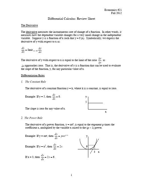
Economics 621 Fall 2012Differential Calculus: Review SheetThe DerivativeThe derivative measures the instantaneous rate of change of a function. In other words, it measures how the dependent variable changes for a very small change in the independent variable. Suppose y is a function of x such that y = f (x). Symbolically, we express the derivative of y with respect to x as:xy l dx dy x ∆∆=→∆0imit The derivative of y with respect to x is equal to the limit of the ratio xy ∆∆ as x ∆approaches zero. That is, the derivative of y is a function that can be used to evaluate the slope of the function, y, for any particular value of x.Differentiation Rules1. The Constant RuleThe derivative of a constant function y = k, where k is a constant, is equal to zero. Example: If y = 5, then 0=dxdy . y 5The slope is zero for any value of x.x2. The Power RuleThe derivative of a power function, y = ax p , is equal to the exponent p times the coefficient a, multiplied by the variable x raised to the (p – 1) power.Example: If y = ax p , then 1-=p pax dxdy yExample: If y = x 2, then x dxdy 2= 9 3 xIf x = 3, then 62==x dxdy .3. The Sum and Difference RulesThe derivative of a linear combination is equal to the sum (difference) of the derivatives of the individual functions.Example: If y = 9x 2 – 2x + 3, then 218-=x dxdy The Partial DerivativeThe derivatives above have been calculated using functions of a singleindependent variable such as y = f (x). Functions of more than one variable are also frequently used in economic analysis such as y = f (x, z). The partial derivative is used to measure the effect that a single independent variable has on the dependent variable in a multivariable function. That is, the partial derivative measures the instantaneous rate of change of the dependent variable (y) with respect to one of the independent variables (x), while the other independentvariable or variables (z) are assumed to be held constant.The partial derivative of y with respect to x for a multivariable function y = f (x, z) can be written as xy ∂∂. Partial differentiation follows all of the same rules listed above by treating all other independent variables as constants.Example: If y = 5x 3 + 3xz + 4z 2, then z x x y 3152+=∂∂ and z x zy 83+=∂∂.Example: If U = 3x 2y 3, then 36xy x U =∂∂ and 229y x yU =∂∂. The Differential The derivative, dxdy , may be treated as the ratio of differentials in which dy is the differential of y and dx is the differential of x. The differential of y measures the changein y resulting from a small change in x. Thus, if y = 2x 2 + 5x + 4, then dxdy = 4x + 5. Multiplying both sides by dx, the differential of y may be expressed as dy = (4x + 5) dx.1. The Total DifferentialFor a function of two or more variables, the total differential measures the change in the dependent variable caused by a small change in each of the independent variables. If y = f (x, z), the total differential is dy = dz z y dx x y ∂∂+∂∂. Example: If y = x 4 + 8xz + 3z 3, then dy = (4x 3 + 8z) dx + (8x + 9z 2) dz.。