Matlab程序代码
遗传算法matlab程序代码
遗传算法matlab程序代码
遗传算法(GA)是一种用于求解优化问题的算法,其主要思想是模拟
生物进化过程中的“选择、交叉、变异”操作,通过模拟这些操作,来寻
找最优解。
Matlab自带了GA算法工具箱,可以直接调用来实现遗传算法。
以下是遗传算法Matlab程序代码示例:
1.初始化
首先定义GA需要优化的目标函数f,以及GA算法的相关参数,如种
群大小、迭代次数、交叉概率、变异概率等,如下所示:
options = gaoptimset('PopulationSize',10,...
'Generations',50,...
2.运行遗传算法
运行GA算法时,需要调用MATLAB自带的ga函数,将目标函数、问
题的维度、上下界、约束条件和算法相关参数作为输入参数。
其中,上下
界和约束条件用于限制空间,防止到无效解。
代码如下:
[某,fval,reason,output,population] = ga(f,2,[],[],[],[],[-10,-10],[10,10],[],options);
3.结果分析
最后,将结果可视化并输出,可以使用Matlab的plot函数绘制出目
标函数的值随迭代次数的变化,如下所示:
plot(output.generations,output.bestf)
某label('Generation')
ylabel('Best function value')
总之,Matlab提供了方便易用的GA算法工具箱,开发者只需要根据具体问题定义好目标函数和相关参数,就能够在短时间内快速实现遗传算法。
一、MATLAB之基础入门代码
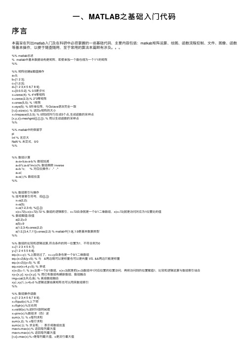
⼀、MATLAB之基础⼊门代码序⾔本篇旨在列出matlab⼊门及在科研中必须掌握的⼀些基础代码,主要内容包括:matkab矩阵运算、绘图、函数流程控制、⽂件、图像、函数等基本操作,以便于随查随⽤,⾄于常⽤的算法本篇鲜有涉及。
%% matlab总述% matlab中基本数据结构是矩阵,即使单独⼀个数也视为⼀个1*1的矩阵%%%% 矩阵创建&赋值操作a=5;b=[1 2 3];c=[1;2;3];d=[1 2 3;4 5 6;7 8 9];x=[0:0.5:2]; % 0.5是步长x=zeros(4); % 4*4零矩阵x=zeros(2,3);% 2*3零矩阵x=ones(5,5); % 1矩阵x=eye(5); % 5阶单位阵,与Octave语法完全⼀致[r,c]=size(x); % 返回x矩阵的⼤⼩x=linspace(0,3,5); % 0到3间均匀⽣成5个点,⽣成函数的采样点[x,y,z]=meshgrid([],[],[]); % ⽤以⽣成函数的采样点%%%% matlab中的保留字piInf % ⽆穷⼤NaN % 未定式,0/0%%%% 数组计算a=a+b;a=a-b;% 数组加减a=b*c;a=b*inv(x)% 数组乘除 inversea=b.*c; % 对应位操作./ .* .^a=a';a=a(:);% 数组拉直%%%% 数组索引与操作% 括号是索引符号,如([],[])x=a(2,2);x=a(5);x=a(1:2,3:4); %([],[])x(x>72)=x(x>72)-72 % 数组的逻辑索引,x>72⾃⾝就是⼀个0/1⼆维数组,x(x>72)就是访问对应为1位置处的值% 数组赋值/改值a(2,2)=0a(5)=9a(1:2,3:4)=ones(2,2)a(1:2,[3,4,7,11])=ones(2,2) % matlab中[1:9],1:9是基本数据类型%%%% 数组的⽐较和逻辑运算,符合条件的同⼀位置为1,不符合则为0x=[1 2 3 4 5 6 7];y=[1 2 4 5 5 6 8];eq=(x==y); %上⾯说过了,x==y⾃⾝也是⼀个0/1⼆维数组eq=(x>2)&(y<5); % 与 &两边既可以是标量也可以是向量 VS. &&两边只能是标量eq=(x>2)|(y<5); % 或eq=xor(x>4,y<5); % 异或x(x<3)=-1; % (x<3)是⼀个0/1数组,x(x<3)就是把(x<3)数组中1对应位置的位置访问,再将访问到的位置赋值1,⽐较和逻辑运算与数组索引结合xy=[x,y]; xy=[x;y]; % ⽤已有数组构建新数组,数组融合img=cat(3,R,G,B); % ⾼级数组融合xy(:,xy(1,:)<4)=0 %逻辑运算结果矩阵也可以⽤来数组索引%%%% 数组操作函数x=[1 2 3;4 5 6;7 8 9];x=flipud(x);%上下转x=fliplr(x);%左右转x=rot90(x);%逆时针旋转90度x=pinv(x);%数组求(伪)逆sum(x,1); % x每列求和sum(x,2); % x每⾏求和sum(x(:)); % 求全和,:表⽰将数组拉直maxn=max(x);% 返回每列最⼤值maxn=max(x);% 返回每列最⼤值maxn=max(x(:)); % 返回全局最⼤值min(); % ⽤法同max()%%%% 常⽤数学函数% 注意matlab中矩阵是基本数据结构,因此所有函数都是对矩阵中每个x_i操作y=sin(x);y=abs(x);%绝对值y=sqrt(x);%开⽅y=ceil(x);%向上取整y=floor(x);%向上取整y=round(x);%四舍五⼊取整y=rand(r,c);%⽣成随机矩阵b=sum(a,idm);%求和函数,dim=1 表⽰对每⼀列求和,dim=2 表⽰对每⼀⾏求和tabulate(detect_result)% detect_result是⼀个列向量,该函数⽤以频数、频率统计%%%% MATLAB函数基本语句for i=1:2:100 %endwhile 1if a<1breakendendfunction [output1,]=functionname(input1,) % 函数定义command1command2output1=%%%% 基本绘图%plotx=0:0.001*pi:2*pi;y=sin(x);z=cos(x);plot(x,y,'-ob','LineWidth',1.5) % 标出数据点的折线图hold onplot(x,z,'rs') % 散点图drawnow % 动画图xlabel('x')ylabel('y')title('图')axis equal % 两轴单位长度相等axis([-2,2,-2,2]) % 控制坐标轴范围set(gca,'XTick',0:pi/2:4*pi); % 设置坐标轴刻度间距,⼀般与下⼀⾏命令搭配set(gca,'XTickLabel',{'0','0.5*pi','pi','1.5*pi','2*pi','2.5*pi','3*pi','3.5*pi','4*pi'})% 设置坐标轴刻度标号xlim([-2,2]) % 控制坐标轴范围text(0,0,'(0,0)') % 在数据曲线上点(x,y)处,标出'(3,5)'legend('cos(x)','sin(x)','sin(x)-cos(x)') % 依照绘图的顺序依次标注图例saveas(gcf,strcat('ch',num2str(i),'.emf')) % 保存plot图⽚,gcf是plot的句柄plot(X)%绘制⼆维矩阵,以⾏号为横坐标,各列为纵坐标plot(X);% plot制作动图for k=1:10plot (fft(eye(k+10))) % eye()单位阵,fft()傅⾥叶变换,plot()绘制矩阵axis equalM(k)=getframe; % 截取当前窗⼝作为影⽚帧endmovie(M,50) %播放多帧图⽚,M 50次%极坐标plar(theta,r,LineSpec)t=0:0.1:3*pi;polar(t,abs(cos(5*t)));% 快速⽅程绘图fplot('x-cos(x^2)',[-4,4]);% 绘制y=x-cos(x^2)ezplot('y-f(x),[-6 6 -8 8]');% ezplot('⽅程式',[xmin xmax ymin ymax])ezplot('cos(3*t)','sin(3*t)',[0:2*pi]);% ezplot('x参数式','y参数式',[tmin,tmax])%%%% 参数⽅程作图(可以画出很有趣的⾮函数图像)t=0:pi/50:2*pi;x=sin(t);y=cos(t);plot(x,y)axis([-1.1,1.1,-1.1,1.1])axis equal%%%%x=sin(t)y=cos(t)z=tplot3(x,y,z) % 三维曲线参数⽅程作图grid on % 开⽹格%%%%三维曲⾯[x,y]=meshgrid(-pi:0.1:pi); % 画函数采样点z=sin(x).*cos(y);mesh(x,y,z) % 画三维曲⾯figure() % 开新画板surf(x,y,z) % 画中间插值的三维曲⾯(有渲染效果)%%%% ⽂件数据读取% .txt纯数据⽂件⽂件data=load('c:\desktop\score.txt')% .txt⽂本⽂件fid=fopen('score.txt','r')line1=fgetl(fid)%数据按分割%数据类型转换line2=fgetl(fid)fclose(fid);fid=fopen('score.txt','w')fprintf(fid,'会当凌绝顶’)fprintf(fid,'%d⽉⼯资 %6.1f\n',[1,2,3,4;20000,19999,20010,25000,23000])fclose(fid);% excel⽂件data=xlsread('filename.xls','Sheet1','A3:C6');data(isnan(data))=0;%空位补零xlswrite('filename.xls',{'t','w'},'Sheet1','B1:C1')%图⽚⽂件img=imread('leave.jpg')% 图⽚读取image(img) % 图⽚显⽰lip(234:435,112:300,:)%图⽚切⽚imshow(lip) % 图⽚显⽰imwrite(img,'c:\\desktop\\figure.emf')% UI交互式导⼊图⽚[FileName PathName FilterIndex]=uigetfile({'*.jpg','*.bmf'},'请导⼊图⽚','*.jpg','MultiSelect','on') if ~ FilterIndexreturnend%视频⽂件data=VideoReader('sport.avi')% data是⼀结构体frame=read(data,25)% 读取视屏中的某⼀帧,即图⽚imshow(frame)% 对视频处理就是循环处理每⼀帧%%%% 线性⽅程求解、拟合、回归x=A\B%⼀元线性拟合x=[2.410 2.468 2.529 2.571 2.618 2.662 2.715 2.747 2.907 2.959 2.997];y=[0 0.800 1.695 2.290 2.965 3.595 4.365 4.810 7.125 7.890 8.425];a=polyfit(x,y,1)%⼀阶拟合 y=a1 x+ a2y=polyval(a,x) % 获得拟合表达式%⾃定义拟合p=fittype('a*x+b*sin(x)+c');% 指定拟合模型f=fit(x,y,p)% 获得拟合函数,x和y必须为列向量plot(f,x,y)% 画出拟合图%差值 x=[1:10] y=[1:10],线性回归求xi对应的yiyi=interp1(x,y,xi,'linear');%线性回归 y=f(x1,x2,x3)%%%%微分⽅程求解%解析解syms y(x);ode=diff(y,x)-y==0;init=y(0)==1;dsolve(ode,init)%dsolve('D2y+4*Dy+24*y=0','y(0)=0,Dy(0)=15','x')%尤克—库塔数值解%%% 符号对象的创建,matlab中之前都是数值计算,这⾥是符号运算a=sym([1/2 sqrt(5)]);y=sym('2*sin(x)*cos(x)');y=simple(y);syms x y;z=cos(x)*sin(y);% 符号表达式及函数的创建, matlab默认是数值运算,符号运算需要提前声明。
matlab经典代码大全
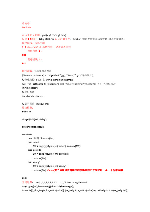
哈哈哈MATLAB显示正炫余炫图:plot(x,y1,'* r',x,y2,'o b')定义【0,2π;t=0:pi/10:2*pi; 定义函数文件:function [返回变量列表]=函数名(输入变量列表) 顺序结构:选择结构1)if-else-end 语句其格式为:if 逻辑表达式程序模块 1 ;else程序模块 2 ;End图片读取:%选择图片路径[filename, pathname] = ... uigetfile({'*.jpg';'*.bmp';'*.gif'},'选择图片');% 合成路径+ 文件名str=[pathname,filename];%为什么pathname 和filename 要前面出现的位置相反才能运行呢???%读取图片im=imread(str);% 使用图片axes(handles.axes1);% 显示图片imshow(im);边缘检测:global imstr=get(hObject,'string');axes (handles.axes1);switch strcase ' 原图' imshow(im);case 'sobel'BW = edge(rgb2gray(im),'sobel'); imshow(BW);case 'prewitt'BW = edge(rgb2gray(im),'prewitt');imshow(BW);case 'canny'BW = edge(rgb2gray(im),'canny');imshow(BW); Canny 算子边缘定位精确性和抗噪声能力效果较好,是一个折中方案end;开闭运算:se=[1,1,1;1,1,1;1,1,1;1,1,1]; %Structuring ElementI=rgb2gray(im); imshow(I,[]);title('Original Image');I=double(I); [im_height,im_width]=size(I); [se_height,se_width]=size(se); halfheight=floor(se_height/2);halfwidth=floor(se_width/2);[se_origin]=floor((size(se)+1)/2); image_dilation=padarray(I,se_origin,0,'both'); %Image to be used for dilation image_erosion=padarray(I,se_origin,256,'both'); %Image to be used forerosion %%%%%%%%%%%%%%%%%%%%% Dilation %%%%%%%%%%%%%%%%%%%%%for k=se_origin(1)+1:im_height+se_origin(1)for kk=se_origin(2)+1:im_width+se_origin(2)dilated_image(k-se_origin(1),kk-se_origin(2))=max(max(se+image_dilation(k-se_origin(1):k+halfh eight-1,kk-se_origin(2):kk+halfwidth-1)));endend figure;imshow(dilated_image,[]);title('Image after Dilation'); %%%%%%%%%%%%%%%%% %%% Erosion %%%%%%%%%%%%%%%%%%%%se=se';for k=se_origin(2)+1:im_height+se_origin(2)for kk=se_origin(1)+1:im_width+se_origin(1)eroded_image(k-se_origin(2),kk-se_origin(1))=min(min(image_erosion(k-se_origin(2):k+halfwidth -1,kk-se_origin(1):kk+halfheight-1)-se));endend figure;imshow(eroded_image,[]);title('Image afterErosion'); %%%%%%%%%%%%%%%%%%%%%%%%%%%%%%%%%%%%%%%%%%%%%%% %%% Opening(Erosion first, thenDilation) %%% %%%%%%%%%%%%%%%%%%%%%%%%%%%%%%%%%%%%%%%%%%%%%%%se=se';image_dilation2=eroded_image; %Image to be used for dilationfor k=se_origin(1)+1:im_height-se_origin(1)for kk=se_origin(2)+1:im_width-se_origin(2)opening_image(k-se_origin(1),kk-se_origin(2))=max(max(se+image_dilation2(k-se_origin(1):k+hal fheight-1,kk-se_origin(2):kk+halfwidth-1)));endend figure;imshow(opening_image,[]);title('OpeningImage'); %%%%%%%%%%%%%%%%%%%%%%%%%%%%%%%%%%%%%%%%%%%%%%% %%% Closing(Dilation first, then Erosion) %%% %%%%%%%%%%%%%%%%%%%%%%%%%%%%%%%%%%%%%%%%%%%%%%% se=se';image_erosion2=dilated_image; %Image to be used for erosionfor k=se_origin(2)+1:im_height-se_origin(2)for kk=se_origin(1)+1:im_width-se_origin(1)closing_image(k-se_origin(2),kk-se_origin(1))=min(min(image_erosion2(k-se_origin(2):k+halfwidt h-1,kk-se_origin(1):kk+halfheight-1)-se));endend figure;imshow(closing_image,[]);title('Closing Image'); Warning: Image is too big to fit on screen; displaying at 31% scale.> In truesize>Resize1 at 308In truesize at 44In imshow at 161 图像的直方图归一化:I=imread(‘red.bmp');%读入图像figure;%打开新窗口[M,N]=size(I);%计算图像大小[counts,x]=imhist(I,32);%计算有32 个小区间的灰度直方图counts=counts/M/N;%计算归一化灰度直方图各区间的值stem(x,counts);%绘制归一化直方图图像平移:I=imread('shuichi.jpg');se=translate(strel(1),[180 190]);B=imdilate(I,se); figure;subplot(1,2,1),subimage(I);title('原图像'); subplot(1,2,2),subimage(B);title('平移后图像');图像的转置;A=imread('nir.bmp'); tform=maketform('affine',[0 1 0;1 0 0;0 0 1]);B=imtransform(A,tform,'nearest');figure;imshow(A);figure;imshow(B);imwrite(B,'nir 转置后图像.bmp');图像滤波:B = imfilter(A,H,option1,option2,...)或写作g = imfilter(f, w, filtering_mode, boundary_options, size_options)其中,f 为输入图像,w 为滤波掩模,g 为滤波后图像。
遗传算法matlab程序代码
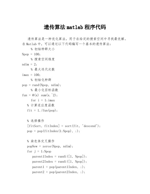
遗传算法matlab程序代码遗传算法是一种优化算法,用于在给定的搜索空间中寻找最优解。
在Matlab中,可以通过以下代码编写一个基本的遗传算法:% 初始种群大小Npop = 100;% 搜索空间维度ndim = 2;% 最大迭代次数imax = 100;% 初始化种群pop = rand(Npop, ndim);% 最小化目标函数fun = @(x) sum(x.^2);for i = 1:imax% 计算适应度函数fit = 1./fun(pop);% 选择操作[fitSort, fitIndex] = sort(fit, 'descend');pop = pop(fitIndex(1:Npop), :);% 染色体交叉操作popNew = zeros(Npop, ndim);for j = 1:Npopparent1Index = randi([1, Npop]);parent2Index = randi([1, Npop]);parent1 = pop(parent1Index, :);parent2 = pop(parent2Index, :);crossIndex = randi([1, ndim-1]);popNew(j,:) = [parent1(1:crossIndex),parent2(crossIndex+1:end)];end% 染色体突变操作for j = 1:NpopmutIndex = randi([1, ndim]);mutScale = randn();popNew(j, mutIndex) = popNew(j, mutIndex) + mutScale;end% 更新种群pop = [pop; popNew];end% 返回最优解[resultFit, resultIndex] = max(fit);result = pop(resultIndex, :);以上代码实现了一个简单的遗传算法,用于最小化目标函数x1^2 + x2^2。
matlab加工自由曲面程序代码
一、引言Matlab是一种高级技术计算语言和交互环境,被广泛用于工程、科学和数学领域的计算与模拟。
在Matlab中,加工自由曲面是一项常见的任务,例如创建和修改三维曲面模型。
本文将介绍如何使用Matlab 编写程序代码来加工自由曲面,以实现对曲面的精确控制和调整。
二、准备工作在编写程序代码之前,首先需要明确自由曲面的定义和参数化方法。
自由曲面通常由参数方程或控制点构成,对于不同的曲面类型,需要选择合适的参数化方法。
还需要了解Matlab中与曲面加工相关的函数和工具,以便在编写程序时能够调用这些资源。
三、编写程序代码1. 定义自由曲面在Matlab中,可以使用符号变量和代数表达式定义自由曲面的参数方程。
对于二次曲面,可以使用二次多项式表示其参数方程。
具体代码如下:syms u vx = a*u^2 + b*v^2 + c*u*v + d*u + e*v + f;y = g*u^2 + h*v^2 + i*u*v + j*u + k*v + l;z = m*u^2 + n*v^2 + o*u*v + p*u + q*v + r;其中a-r为曲面的系数,u和v为曲面的参数。
2. 控制曲面形状通过调整曲面的参数和系数,可以控制曲面的形状。
可以通过改变系数a-r的值来实现对曲面的放大缩小、旋转、偏移等操作。
具体代码如下:a = 1;b = 1;c = 0;d = 0;e = 0;f = 0;g = 1; h = 1; i = 0; j = 0; k = 0; l = 0;m = 1; n = 1; o = 0; p = 0; q = 0; r = 0;这里以简单的二次曲面为例,通过调整系数的数值来控制曲面的形状。
3. 曲面绘制和可视化在定义和控制曲面之后,可以使用Matlab中的绘图函数将曲面绘制出来。
可以使用surf函数创建曲面图形,并通过设置图形属性来进行可视化调整。
具体代码如下:[u, v] = meshgrid(-2:0.1:2);x = a*u.^2 + b*v.^2 + c*u.*v + d*u + e*v + f;y = g*u.^2 + h*v.^2 + i*u.*v + j*u + k*v + l;z = m*u.^2 + n*v.^2 + o*u.*v + p*u + q*v + r;surf(x, y, z);四、应用实例在实际应用中,自由曲面加工可以用于创建各种复杂的曲面模型。
matlab经典代码大全

哈哈哈MATLAB显示正炫余炫图:plot(x,y1,'* r',x,y2,'o b')定义【0,2π】;t=0:pi/10:2*pi;定义函数文件:function [返回变量列表]=函数名(输入变量列表)顺序结构:选择结构1)if-else-end语句其格式为:if 逻辑表达式程序模块1;else程序模块2;End图片读取:%选择图片路径[filename, pathname] = ...uigetfile({'*.jpg';'*.bmp';'*.gif'},'选择图片');%合成路径+文件名str=[pathname,filename];%为什么pathname和filename要前面出现的位置相反才能运行呢???%读取图片im=imread(str);%使用图片axes(handles.axes1);%显示图片imshow(im);边缘检测:global imstr=get(hObject,'string');axes (handles.axes1);switch strcase ' 原图'imshow(im);case 'sobel'BW = edge(rgb2gray(im),'sobel');imshow(BW);case 'prewitt'BW = edge(rgb2gray(im),'prewitt');imshow(BW);case 'canny'BW = edge(rgb2gray(im),'canny');imshow(BW);Canny算子边缘定位精确性和抗噪声能力效果较好,是一个折中方案end;开闭运算:se=[1,1,1;1,1,1;1,1,1;1,1,1]; %Structuring ElementI=rgb2gray(im);imshow(I,[]);title('Original Image');I=double(I);[im_height,im_width]=size(I);[se_height,se_width]=size(se);halfheight=floor(se_height/2);halfwidth=floor(se_width/2);[se_origin]=floor((size(se)+1)/2);image_dilation=padarray(I,se_origin,0,'both'); %Image to be used for dilationimage_erosion=padarray(I,se_origin,256,'both'); %Image to be used for erosion %%%%%%%%%%%%%%%%%%%%% Dilation %%%%%%%%%%%%%%%%%%%%%for k=se_origin(1)+1:im_height+se_origin(1)for kk=se_origin(2)+1:im_width+se_origin(2)dilated_image(k-se_origin(1),kk-se_origin(2))=max(max(se+image_dilation(k-se_origin(1):k+halfh eight-1,kk-se_origin(2):kk+halfwidth-1)));endendfigure;imshow(dilated_image,[]);title('Image after Dilation'); %%%%%%%%%%%%%%%%%%%% Erosion %%%%%%%%%%%%%%%%%%%%se=se';for k=se_origin(2)+1:im_height+se_origin(2)for kk=se_origin(1)+1:im_width+se_origin(1)eroded_image(k-se_origin(2),kk-se_origin(1))=min(min(image_erosion(k-se_origin(2):k+halfwidth -1,kk-se_origin(1):kk+halfheight-1)-se));endendfigure;imshow(eroded_image,[]);title('Image after Erosion'); %%%%%%%%%%%%%%%%%%%%%%%%%%%%%%%%%%%%%%%%%%%%%%%%%% Opening(Erosion first, then Dilation) %%% %%%%%%%%%%%%%%%%%%%%%%%%%%%%%%%%%%%%%%%%%%%%%%%se=se';image_dilation2=eroded_image; %Image to be used for dilationfor k=se_origin(1)+1:im_height-se_origin(1)for kk=se_origin(2)+1:im_width-se_origin(2)opening_image(k-se_origin(1),kk-se_origin(2))=max(max(se+image_dilation2(k-se_origin(1):k+hal fheight-1,kk-se_origin(2):kk+halfwidth-1)));endendfigure;imshow(opening_image,[]);title('Opening Image'); %%%%%%%%%%%%%%%%%%%%%%%%%%%%%%%%%%%%%%%%%%%%%%%%%% Closing(Dilation first, then Erosion) %%% %%%%%%%%%%%%%%%%%%%%%%%%%%%%%%%%%%%%%%%%%%%%%%%se=se';image_erosion2=dilated_image; %Image to be used for erosionfor k=se_origin(2)+1:im_height-se_origin(2)for kk=se_origin(1)+1:im_width-se_origin(1)closing_image(k-se_origin(2),kk-se_origin(1))=min(min(image_erosion2(k-se_origin(2):k+halfwidt h-1,kk-se_origin(1):kk+halfheight-1)-se));endendfigure;imshow(closing_image,[]);title('Closing Image');Warning: Image is too big to fit on screen; displaying at 31% scale.> In truesize>Resize1 at 308In truesize at 44In imshow at 161图像的直方图归一化:I=imread(‘red.bmp’);%读入图像figure;%打开新窗口[M,N]=size(I);%计算图像大小[counts,x]=imhist(I,32);%计算有32个小区间的灰度直方图counts=counts/M/N;%计算归一化灰度直方图各区间的值stem(x,counts);%绘制归一化直方图图像平移:I=imread('shuichi.jpg');se=translate(strel(1),[180 190]);B=imdilate(I,se);figure;subplot(1,2,1),subimage(I);title('原图像');subplot(1,2,2),subimage(B);title('平移后图像');图像的转置;A=imread('nir.bmp');tform=maketform('affine',[0 1 0;1 0 0;0 0 1]);B=imtransform(A,tform,'nearest');figure;imshow(A);figure;imshow(B);imwrite(B,'nir转置后图像.bmp');图像滤波:B = imfilter(A,H,option1,option2,...)或写作g = imfilter(f, w, filtering_mode, boundary_options, size_options)其中,f为输入图像,w为滤波掩模,g为滤波后图像。
Matlab100个实例程序
程序代码:(代码标记[code]...[/code] ) 1-32是:图形应用篇33-66是:界面设计篇67-84是:图形处理篇85-100是:数值分析篇实例1:三角函数曲线(1)function shili01h0=figure('toolbar','none',...'position',[198****0300],...'name','实例01');h1=axes('parent',h0,...'visible','off');x=-pi:0.05:pi;y=sin(x);plot(x,y);xlabel('自变量X');ylabel('函数值Y');title('SIN( )函数曲线');grid on实例2:三角函数曲线(2)function shili02h0=figure('toolbar','none',...'position',[200 150 450 350],...'name','实例02');x=-pi:0.05:pi;y=sin(x)+cos(x);plot(x,y,'-*r','linewidth',1);grid onxlabel('自变量X');ylabel('函数值Y');title('三角函数');实例3:图形的叠加function shili03h0=figure('toolbar','none',...'position',[200 150 450 350],...'name','实例03');x=-pi:0.05:pi;y1=sin(x);y2=cos(x);plot(x,y1,...'-*r',...x,y2,...'--og');grid onxlabel('自变量X');ylabel('函数值Y');title('三角函数');实例4:双y轴图形的绘制function shili04h0=figure('toolbar','none',...'position',[200 150 450 250],...'name','实例04');x=0:900;a=1000;b=0.005;y1=2*x;y2=cos(b*x);[haxes,hline1,hline2]=plotyy(x,y1,x,y2,'semilogy','plot'); axes(haxes(1))ylabel('semilog plot');axes(haxes(2))ylabel('linear plot');实例5:单个轴窗口显示多个图形function shili05h0=figure('toolbar','none',...'position',[200 150 450 250],...'name','实例05');t=0:pi/10:2*pi;[x,y]=meshgrid(t);subplot(2,2,1)plot(sin(t),cos(t))axis equalsubplot(2,2,2)z=sin(x)-cos(y);plot(t,z)axis([0 2*pi -2 2])subplot(2,2,3)h=sin(x)+cos(y);plot(t,h)axis([0 2*pi -2 2])subplot(2,2,4)g=(sin(x).^2)-(cos(y).^2);plot(t,g)axis([0 2*pi -1 1])实例6:图形标注function shili06h0=figure('toolbar','none',...'position',[200 150 450 400],...'name','实例06');t=0:pi/10:2*pi;h=plot(t,sin(t));xlabel('t=0到2\pi','fontsize',16);ylabel('sin(t)','fontsize',16);title('\it{从0to2\pi 的正弦曲线}','fontsize',16) x=get(h,'xdata');y=get(h,'ydata');imin=find(min(y)==y);imax=find(max(y)==y);text(x(imin),y(imin),...['\leftarrow最小值=',num2str(y(imin))],... 'fontsize',16)text(x(imax),y(imax),...['\leftarrow最大值=',num2str(y(imax))],...'fontsize',16)实例7:条形图形function shili07h0=figure('toolbar','none',...'position',[200 150 450 350],...'name','实例07');tiao1=[562 548 224 545 41 445 745 512];tiao2=[47 48 57 58 54 52 65 48];t=0:7;bar(t,tiao1)xlabel('X轴');ylabel('TIAO1值');h1=gca;h2=axes('position',get(h1,'position'));plot(t,tiao2,'linewidth',3)set(h2,'yaxislocation','right','color','none','xticklabel',[])实例8:区域图形function shili08h0=figure('toolbar','none',...'position',[200 150 450 250],...'name','实例08');x=91:95;profits1=[88 75 84 93 77];profits2=[51 64 54 56 68];profits3=[42 54 34 25 24];profits4=[26 38 18 15 4];area(x,profits1,'facecolor',[0.5 0.9 0.6],...'edgecolor','b',...'linewidth',3)hold onarea(x,profits2,'facecolor',[0.9 0.85 0.7],...'edgecolor','y',...'linewidth',3)hold onarea(x,profits3,'facecolor',[0.3 0.6 0.7],... 'edgecolor','r',...'linewidth',3)hold onarea(x,profits4,'facecolor',[0.6 0.5 0.9],... 'edgecolor','m',...'linewidth',3)hold offset(gca,'xtick',[91:95])set(gca,'layer','top')gtext('\leftarrow第一季度销量')gtext('\leftarrow第二季度销量')gtext('\leftarrow第三季度销量')gtext('\leftarrow第四季度销量')xlabel('年','fontsize',16);ylabel('销售量','fontsize',16);实例9:饼图的绘制function shili09h0=figure('toolbar','none',...'position',[200 150 450 250],...'name','实例09');t=[54 21 35;68 54 35;45 25 12;48 68 45;68 54 69];x=sum(t);h=pie(x);textobjs=findobj(h,'type','text');str1=get(textobjs,{'string'});val1=get(textobjs,{'extent'});oldext=cat(1,val1{:});names={'商品一:';'商品二:';'商品三:'}; str2=strcat(names,str1);set(textobjs,{'string'},str2)val2=get(textobjs,{'extent'});newext=cat(1,val2{:});offset=sign(oldext(:,1)).*(newext(:,3)-oldext(:,3))/2; pos=get(textobjs,{'position'});textpos=cat(1,pos{:});textpos(:,1)=textpos(:,1)+offset;set(textobjs,{'position'},num2cell(textpos,[3,2]))实例10:阶梯图function shili10h0=figure('toolbar','none',...'position',[200 150 450 400],...'name','实例10');a=0.01;b=0.5;t=0:10;f=exp(-a*t).*sin(b*t);stairs(t,f)hold onplot(t,f,':*')hold offglabel='函数e^{-(\alpha*t)}sin\beta*t的阶梯图'; gtext(glabel,'fontsize',16)xlabel('t=0:10','fontsize',16)axis([0 10 -1.2 1.2])实例11:枝干图function shili11h0=figure('toolbar','none',...'position',[200 150 450 350],...'name','实例11');x=0:pi/20:2*pi;y1=sin(x);y2=cos(x);h1=stem(x,y1+y2);hold onh2=plot(x,y1,'^r',x,y2,'*g');h3=[h1(1);h2];legend(h3,'y1+y2','y1=sin(x)','y2=cos(x)') xlabel('自变量X');ylabel('函数值Y');title('正弦函数与余弦函数的线性组合');实例12:罗盘图function shili12h0=figure('toolbar','none',...'position',[200 150 450 250],...'name','实例12');winddirection=[54 24 65 84256 12 235 62125 324 34 254];windpower=[2 5 5 36 8 12 76 14 10 8];rdirection=winddirection*pi/180;[x,y]=pol2cart(rdirection,windpower); compass(x,y);desc={'风向和风力','北京气象台','10月1日0:00到','10月1日12:00'};gtext(desc)实例13:轮廓图function shili13h0=figure('toolbar','none',...'position',[200 150 450 250],...'name','实例13');[th,r]=meshgrid((0:10:360)*pi/180,0:0.05:1); [x,y]=pol2cart(th,r);z=x+i*y;f=(z.^4-1).^(0.25);contour(x,y,abs(f),20)xlabel('实部','fontsize',16);ylabel('虚部','fontsize',16);h=polar([0 2*pi],[0 1]);delete(h)hold oncontour(x,y,abs(f),20)实例14:交互式图形function shili14h0=figure('toolbar','none',...'position',[200 150 450 250],... 'name','实例14');axis([0 10 0 10]);hold onx=[];y=[];n=0;disp('单击鼠标左键点取需要的点'); disp('单击鼠标右键点取最后一个点'); but=1;while but==1[xi,yi,but]=ginput(1);plot(xi,yi,'bo')n=n+1;disp('单击鼠标左键点取下一个点'); x(n,1)=xi;y(n,1)=yi;endt=1:n;ts=1:0.1:n;xs=spline(t,x,ts);ys=spline(t,y,ts);plot(xs,ys,'r-');hold off实例15:变换的傅立叶函数曲线function shili15h0=figure('toolbar','none',...'position',[200 150 450 250],...'name','实例15');axis equalm=moviein(20,gcf);set(gca,'nextplot','replacechildren')h=uicontrol('style','slider','position',... [100 10 500 20],'min',1,'max',20) for j=1:20plot(fft(eye(j+16)))set(h,'value',j)m(:,j)=getframe(gcf);endclf;axes('position',[0 0 1 1]);movie(m,30)实例16:劳伦兹非线形方程的无序活动function shili15h0=figure('toolbar','none',...'position',[200 150 450 250],...'name','实例15');axis equalm=moviein(20,gcf);set(gca,'nextplot','replacechildren')h=uicontrol('style','slider','position',... [100 10 500 20],'min',1,'max',20) for j=1:20plot(fft(eye(j+16)))set(h,'value',j)m(:,j)=getframe(gcf);endclf;axes('position',[0 0 1 1]);movie(m,30)实例17:填充图function shili17h0=figure('toolbar','none',...'position',[200 150 450 250],... 'name','实例17');t=(1:2:15)*pi/8;x=sin(t);y=cos(t);fill(x,y,'r')axis square offtext(0,0,'STOP',...'color',[1 1 1],...'fontsize',50,...'horizontalalignment','center')实例18:条形图和阶梯形图function shili18h0=figure('toolbar','none',...'position',[200 150 450 250],... 'name','实例18');subplot(2,2,1)x=-3:0.2:3;y=exp(-x.*x);bar(x,y)title('2-D Bar Chart')subplot(2,2,2)x=-3:0.2:3;y=exp(-x.*x);bar3(x,y,'r')title('3-D Bar Chart')subplot(2,2,3)x=-3:0.2:3;y=exp(-x.*x);stairs(x,y)title('Stair Chart')subplot(2,2,4)x=-3:0.2:3;y=exp(-x.*x);barh(x,y)title('Horizontal Bar Chart')实例19:三维曲线图function shili19h0=figure('toolbar','none',...'position',[200 150 450 400],... 'name','实例19');subplot(2,1,1)x=linspace(0,2*pi);y1=sin(x);y2=cos(x);y3=sin(x)+cos(x);z1=zeros(size(x));z2=0.5*z1;z3=z1;plot3(x,y1,z1,x,y2,z2,x,y3,z3) grid onxlabel('X轴');ylabel('Y轴');zlabel('Z轴');title('Figure1:3-D Plot')subplot(2,1,2)x=linspace(0,2*pi);y1=sin(x);y2=cos(x);y3=sin(x)+cos(x);z1=zeros(size(x));z2=0.5*z1;z3=z1;plot3(x,z1,y1,x,z2,y2,x,z3,y3) grid onxlabel('X轴');zlabel('Z轴');title('Figure2:3-D Plot')实例20:图形的隐藏属性function shili20h0=figure('toolbar','none',...'position',[200 150 450 300],... 'name','实例20');subplot(1,2,1)[x,y,z]=sphere(10);mesh(x,y,z)axis offtitle('Figure1:Opaque')hidden onsubplot(1,2,2)[x,y,z]=sphere(10);mesh(x,y,z)axis offtitle('Figure2:Transparent') hidden off实例21:PEAKS函数曲线function shili21h0=figure('toolbar','none',...'position',[200 100 450 450],... 'name','实例21');[x,y,z]=peaks(30);subplot(2,1,1)x=x(1,:);y=y(:,1);i=find(y>0.8&y<1.2);j=find(x>-0.6&x<0.5);z(i,j)=nan*z(i,j);surfc(x,y,z)xlabel('X轴');ylabel('Y轴');title('Figure1:surfc函数形成的曲面')subplot(2,1,2)x=x(1,:);y=y(:,1);i=find(y>0.8&y<1.2);j=find(x>-0.6&x<0.5);z(i,j)=nan*z(i,j);surfl(x,y,z)xlabel('X轴');ylabel('Y轴');zlabel('Z轴');title('Figure2:surfl函数形成的曲面')实例22:片状图function shili22h0=figure('toolbar','none',...'position',[200 150 550 350],...'name','实例22');subplot(1,2,1)x=rand(1,20);y=rand(1,20);z=peaks(x,y*pi);t=delaunay(x,y);trimesh(t,x,y,z)hidden offtitle('Figure1:Triangular Surface Plot');subplot(1,2,2)x=rand(1,20);y=rand(1,20);z=peaks(x,y*pi);t=delaunay(x,y);trisurf(t,x,y,z)title('Figure1:Triangular Surface Plot');实例23:视角的调整function shili23h0=figure('toolbar','none',...'position',[200 150 450 350],... 'name','实例23');x=-5:0.5:5;[x,y]=meshgrid(x);r=sqrt(x.^2+y.^2)+eps;z=sin(r)./r;subplot(2,2,1)surf(x,y,z)xlabel('X-axis')ylabel('Y-axis')zlabel('Z-axis')title('Figure1')view(-37.5,30)subplot(2,2,2)surf(x,y,z)xlabel('X-axis')ylabel('Y-axis')zlabel('Z-axis')title('Figure2')view(-37.5+90,30)subplot(2,2,3)surf(x,y,z)xlabel('X-axis')ylabel('Y-axis')zlabel('Z-axis')title('Figure3')view(-37.5,60)subplot(2,2,4)surf(x,y,z)xlabel('X-axis')ylabel('Y-axis')zlabel('Z-axis')title('Figure4')view(180,0)实例24:向量场的绘制function shili24h0=figure('toolbar','none',...'position',[200 150 450 350],... 'name','实例24');subplot(2,2,1)z=peaks;ribbon(z)title('Figure1')subplot(2,2,2)[x,y,z]=peaks(15);[dx,dy]=gradient(z,0.5,0.5); contour(x,y,z,10)hold onquiver(x,y,dx,dy)hold offtitle('Figure2')subplot(2,2,3)[x,y,z]=peaks(15);[nx,ny,nz]=surfnorm(x,y,z);surf(x,y,z)hold onquiver3(x,y,z,nx,ny,nz)hold offtitle('Figure3')subplot(2,2,4)x=rand(3,5);y=rand(3,5);z=rand(3,5);c=rand(3,5);fill3(x,y,z,c)grid ontitle('Figure4')实例25:灯光定位function shili25h0=figure('toolbar','none',...'position',[200 150 450 250],... 'name','实例25');vert=[1 1 1;1 2 1;2 2 1;2 1 1;1 1 2;12 2;2 2 2;2 1 2];fac=[1 2 3 4;2 6 7 3;4 3 7 8;15 8 4;1 2 6 5;5 6 7 8];grid offsphere(36)h=findobj('type','surface');set(h,'facelighting','phong',...'facecolor',...'interp',...'edgecolor',[0.4 0.4 0.4],...'backfacelighting',...'lit')hold onpatch('faces',fac,'vertices',vert,... 'facecolor','y');light('position',[1 3 2]);light('position',[-3 -1 3]); material shinyaxis vis3d offhold off实例26:柱状图function shili26h0=figure('toolbar','none',...'position',[200 50 450 450],...'name','实例26');subplot(2,1,1)x=[5 2 18 7 39 8 65 5 54 3 2];bar(x)xlabel('X轴');ylabel('Y轴');title('第一子图');subplot(2,1,2)y=[5 2 18 7 39 8 65 5 54 3 2];barh(y)xlabel('X轴');ylabel('Y轴');title('第二子图');实例27:设置照明方式function shili27h0=figure('toolbar','none',...'position',[200 150 450 350],... 'name','实例27');subplot(2,2,1)sphereshading flatcamlight leftcamlight rightlighting flatcolorbaraxis offtitle('Figure1')subplot(2,2,2)sphereshading flatcamlight leftcamlight rightlighting gouraudcolorbaraxis offtitle('Figure2')subplot(2,2,3)sphereshading interpcamlight rightcamlight leftlighting phongcolorbaraxis offtitle('Figure3')subplot(2,2,4)sphereshading flatcamlight leftcamlight rightlighting nonecolorbaraxis offtitle('Figure4')实例28:羽状图function shili28h0=figure('toolbar','none',...'position',[200 150 450 350],... 'name','实例28');subplot(2,1,1)alpha=90:-10:0;r=ones(size(alpha));m=alpha*pi/180;n=r*10;[u,v]=pol2cart(m,n);feather(u,v)title('羽状图')axis([0 20 0 10])subplot(2,1,2)t=0:0.5:10;x=0.05+i;y=exp(-x*t);feather(y)title('复数矩阵的羽状图')实例29:立体透视(1)function shili29h0=figure('toolbar','none',...'position',[200 150 450 250],... 'name','实例29');[x,y,z]=meshgrid(-2:0.1:2,...-2:0.1:2,...-2:0.1:2);v=x.*exp(-x.^2-y.^2-z.^2); grid onfor i=-2:0.5:2;h1=surf(linspace(-2,2,20),...linspace(-2,2,20),...zeros(20)+i);rotate(h1,[1 -1 1],30)dx=get(h1,'xdata');dy=get(h1,'ydata');dz=get(h1,'zdata');delete(h1)slice(x,y,z,v,[-2 2],2,-2)hold onslice(x,y,z,v,dx,dy,dz)hold offaxis tightview(-5,10)drawnowend实例30:立体透视(2)function shili30h0=figure('toolbar','none',...'position',[200 150 450 250],... 'name','实例30');[x,y,z]=meshgrid(-2:0.1:2,...-2:0.1:2,...-2:0.1:2);v=x.*exp(-x.^2-y.^2-z.^2); [dx,dy,dz]=cylinder;slice(x,y,z,v,[-2 2],2,-2)for i=-2:0.2:2h=surface(dx+i,dy,dz);rotate(h,[1 0 0],90)xp=get(h,'xdata');yp=get(h,'ydata');zp=get(h,'zdata');delete(h)hold onhs=slice(x,y,z,v,xp,yp,zp);axis tightxlim([-3 3])view(-10,35)drawnowdelete(hs)hold offend实例31:表面图形function shili31h0=figure('toolbar','none',...'position',[200 150 550 250],...'name','实例31');subplot(1,2,1)x=rand(100,1)*16-8;y=rand(100,1)*16-8;r=sqrt(x.^2+y.^2)+eps;z=sin(r)./r;xlin=linspace(min(x),max(x),33); ylin=linspace(min(y),max(y),33); [X,Y]=meshgrid(xlin,ylin);Z=griddata(x,y,z,X,Y,'cubic'); mesh(X,Y,Z)axis tighthold onplot3(x,y,z,'.','Markersize',20)subplot(1,2,2)k=5;n=2^k-1;theta=pi*(-n:2:n)/n;phi=(pi/2)*(-n:2:n)'/n;X=cos(phi)*cos(theta);Y=cos(phi)*sin(theta);Z=sin(phi)*ones(size(theta)); colormap([0 0 0;1 1 1])C=hadamard(2^k);surf(X,Y,Z,C)axis square实例32:沿曲线移动的小球h0=figure('toolbar','none',...'position',[198****8468],... 'name','实例32');h1=axes('parent',h0,...'position',[0.15 0.45 0.7 0.5],... 'visible','on');t=0:pi/24:4*pi;y=sin(t);plot(t,y,'b')n=length(t);h=line('color',[0 0.5 0.5],...'linestyle','.',...'markersize',25,...'erasemode','xor');k1=uicontrol('parent',h0,...'style','pushbutton',...'position',[80 100 50 30],...'string','开始',...'callback',[...'i=1;',...'k=1;,',...'m=0;,',...'while 1,',...'if k==0,',...'break,',...'end,',...'if k~=0,',...'set(h,''xdata'',t(i),''ydata'',y(i)),',...'drawnow;,',...'i=i+1;,',...'if i>n,',...'m=m+1;,',...'i=1;,',...'end,',...'end,',...'end']);k2=uicontrol('parent',h0,...'style','pushbutton',...'position',[180 100 50 30],...'string','停止',...'callback',[...'k=0;,',...'set(e1,''string'',m),',...'p=get(h,''xdata'');,',...'q=get(h,''ydata'');,',...'set(e2,''string'',p);,',...'set(e3,''string'',q)']);k3=uicontrol('parent',h0,...'style','pushbutton',...'position',[280 100 50 30],... 'string','关闭',...'callback','close');e1=uicontrol('parent',h0,...'style','edit',...'position',[60 30 60 20]);t1=uicontrol('parent',h0,...'style','text',...'string','循环次数',...'position',[60 50 60 20]);e2=uicontrol('parent',h0,...'style','edit',...'position',[180 30 50 20]);t2=uicontrol('parent',h0,...'style','text',...'string','终点的X坐标值',...'position',[155 50 100 20]);e3=uicontrol('parent',h0,...'style','edit',...'position',[300 30 50 20]);t3=uicontrol('parent',h0,...'style','text',...'string','终点的Y坐标值',...'position',[275 50 100 20]);实例33:曲线转换按钮h0=figure('toolbar','none',...'position',[200 150 450 250],... 'name','实例33');x=0:0.5:2*pi;y=sin(x);h=plot(x,y);grid on'if i==1,',...'i=0;,',...'y=cos(x);,',...'delete(h),',...'set(hm,''string'',''正弦函数''),',...'h=plot(x,y);,',...'grid on,',...'else if i==0,',...'i=1;,',...'y=sin(x);,',...'set(hm,''string'',''余弦函数''),',...'delete(h),',...'h=plot(x,y);,',...'grid on,',...'end,',...'end'];hm=uicontrol(gcf,'style','pushbutton',... 'string','余弦函数',...'callback',huidiao);i=1;set(hm,'position',[250 20 60 20]);set(gca,'position',[0.2 0.2 0.6 0.6]) title('按钮的使用')hold on实例34:栅格控制按钮h0=figure('toolbar','none',...'position',[200 150 450 250],...'name','实例34');x=0:0.5:2*pi;y=sin(x);plot(x,y)huidiao1=[...'set(h_toggle2,''value'',0),',...'grid on,',...];'set(h_toggle1,''value'',0),',...'grid off,',...];h_toggle1=uicontrol(gcf,'style','togglebutton',... 'string','grid on',...'value',0,...'position',[20 45 50 20],...'callback',huidiao1);h_toggle2=uicontrol(gcf,'style','togglebutton',... 'string','grid off',...'value',0,...'position',[20 20 50 20],...'callback',huidiao2);set(gca,'position',[0.2 0.2 0.6 0.6])title('开关按钮的使用')实例35:编辑框的使用h0=figure('toolbar','none',...'position',[200 150 350 250],...'name','实例35');f='Please input the letter';huidiao1=[...'g=upper(f);,',...'set(h2_edit,''string'',g),',...];huidiao2=[...'g=lower(f);,',...'set(h2_edit,''string'',g),',...];h1_edit=uicontrol(gcf,'style','edit',...'position',[100 200 100 50],...'HorizontalAlignment','left',...'string','Please input the letter',...'callback','f=get(h1_edit,''string'');',...'background','w',...'max',5,...'min',1);h2_edit=uicontrol(gcf,'style','edit',...'HorizontalAlignment','left',...'position',[100 100 100 50],...'background','w',...'max',5,...'min',1);h1_button=uicontrol(gcf,'style','pushbutton',... 'string','小写变大写',...'position',[100 45 100 20],...'callback',huidiao1);h2_button=uicontrol(gcf,'style','pushbutton',... 'string','大写变小写',...'position',[100 20 100 20],...'callback',huidiao2);实例36:弹出式菜单h0=figure('toolbar','none',...'position',[200 150 450 250],...'name','实例36');x=0:0.5:2*pi;y=sin(x);h=plot(x,y);grid onhm=uicontrol(gcf,'style','popupmenu',...'string',...'sin(x)|cos(x)|sin(x)+cos(x)|exp(-sin(x))',... 'position',[250 20 50 20]);set(hm,'value',1)huidiao=[...'v=get(hm,''value'');,',...'switch v,',...'case 1,',...'delete(h),',...'y=sin(x);,',...'h=plot(x,y);,',...'grid on,',...'case 2,',...'delete(h),',...'y=cos(x);,',...'h=plot(x,y);,',...'grid on,',...'case 3,',...'delete(h),',...'y=sin(x)+cos(x);,',...'h=plot(x,y);,',...'grid on,',...'case 4,',...'delete(h),',...'y=exp(-sin(x));,',...'h=plot(x,y);,',...'grid on,',...'end'];set(hm,'callback',huidiao)set(gca,'position',[0.2 0.2 0.6 0.6]) title('弹出式菜单的使用')实例37:滑标的使用h0=figure('toolbar','none',...'position',[200 150 450 250],... 'name','实例37');[x,y]=meshgrid(-8:0.5:8);r=sqrt(x.^2+y.^2)+eps;z=sin(r)./r;h0=mesh(x,y,z);h1=axes('position',...[0.2 0.2 0.5 0.5],...'visible','off');htext=uicontrol(gcf,...'units','points',...'position',[20 30 45 15],...'string','brightness',...'style','text');hslider=uicontrol(gcf,...'units','points',...'position',[10 10 300 15],...'min',-1,...'max',1,...'style','slider',...'callback',...'brighten(get(hslider,''value''))');实例38:多选菜单h0=figure('toolbar','none',...'position',[200 150 450 250],...'name','实例38');[x,y]=meshgrid(-8:0.5:8);r=sqrt(x.^2+y.^2)+eps;z=sin(r)./r;h0=mesh(x,y,z);hlist=uicontrol(gcf,'style','listbox',...'string','default|spring|summer|autumn|winter',... 'max',5,...'min',1,...'position',[20 20 80 100],...'callback',[...'k=get(hlist,''value'');,',...'switch k,',...'case 1,',...'colormap default,',...'case 2,',...'colormap spring,',...'case 3,',...'colormap summer,',...'case 4,',...'colormap autumn,',...'case 5,',...'colormap winter,',...'end']);实例39:菜单控制的使用h0=figure('toolbar','none',...'position',[200 150 450 250],...'name','实例39');x=0:0.5:2*pi;y=cos(x);h=plot(x,y);grid onset(gcf,'toolbar','none')hm=uimenu('label','example');huidiao1=[...'set(hm_gridon,''checked'',''on''),',...'set(hm_gridoff,''checked'',''off''),',...'grid on'];huidiao2=[...'set(hm_gridoff,''checked'',''on''),',...'set(hm_gridon,''checked'',''off''),',...'grid off'];hm_gridon=uimenu(hm,'label','grid on',... 'checked','on',...'callback',huidiao1);hm_gridoff=uimenu(hm,'label','grid off',... 'checked','off',...'callback',huidiao2);实例40:UIMENU菜单的应用h0=figure('toolbar','none',...'position',[200 150 450 250],...'name','实例40');h1=uimenu(gcf,'label','函数');h11=uimenu(h1,'label','轮廓图',...'callback',[...'set(h31,''checked'',''on''),',...'set(h32,''checked'',''off''),',...'[x,y,z]=peaks;,',...'contour3(x,y,z,30)']);h12=uimenu(h1,'label','高斯分布',...。
matlab程序算例

matlab程序算例Matlab程序算例Matlab是一种广泛应用于科学和工程领域的高级计算机编程语言及环境。
它的简洁、高效和强大的功能使得许多人选择使用Matlab来解决复杂的数学和工程问题。
在本文中,我将以一个具体的Matlab程序算例为例,详细说明每一步是如何完成的。
那么我们首先来看一下这个具体的Matlab程序算例。
假设我们希望计算并绘制一个二维正弦函数,代码如下:matlab设置步长,定义x轴的范围dx = 0.1;x = 0:dx:10;计算对应的y值y = sin(x);绘制图像plot(x, y);在这个例子中,我们通过定义一个步长`dx`和一个x轴的范围`x`来生成一系列的x值。
然后,我们使用`sin()`函数计算对应的y值,并将结果保存在`y`中。
最后,我们使用`plot()`函数绘制x和y的图像。
现在,让我们一步一步来回答这个程序算例中的问题。
第一步:设置步长和定义x轴的范围。
matlabdx = 0.1;x = 0:dx:10;这里我们设置步长`dx`为0.1,表示x轴上两个相邻点之间的间距为0.1。
然后,我们使用冒号运算符`:`创建一个从0到10的向量`x`,其中每个元素之间的间隔为`dx`。
也就是说,`x`中的元素为0, 0.1, 0.2, …, 9.9, 10。
第二步:计算对应的y值。
matlaby = sin(x);这里,我们使用`sin()`函数计算每个x值对应的正弦值,并将结果保存在`y`中。
例如,如果x的第一个元素为0,则使用`sin(0)`计算得到y的第一个元素的值。
第三步:绘制图像。
matlabplot(x, y);最后,我们使用`plot()`函数将x和y的值绘制成图像。
这样就可以观察到x和y之间的关系。
在这个例子中,由于x的范围是从0到10,并且y是对应的正弦值,因此我们将得到一个周期为2π的正弦函数的图像。
以上就是这个Matlab程序算例的每一步的解释。