Acoustic monitoring of gas emissions from the seafloor. Part II
NDT检测词汇-英汉
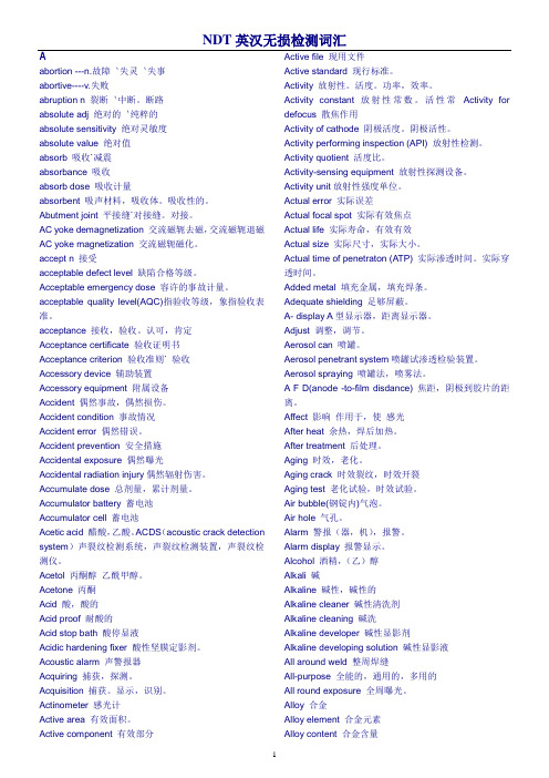
Aabortion ---n.故障`失灵`失事abortive----v.失败abruption n 裂断`中断。
断路absolute adj 绝对的`纯粹的absolute sensitivity 绝对灵敏度absolute value 绝对值absorb 吸收`减震absorbance 吸收absorb dose 吸收计量absorbent 吸声材料,吸收体。
吸收性的。
Abutment joint 平接缝`对接缝。
对接。
AC yoke demagnetization 交流磁轭去磁,交流磁轭退磁AC yoke magnetization 交流磁轭磁化。
accept n 接受acceptable defect level 缺陷合格等级。
Acceptable emergency dose 容许的事故计量。
acceptable quality level(AQC)指验收等级,象指验收表准。
acceptance 接收,验收。
认可,肯定Acceptance certificate 验收证明书Acceptance criterion 验收准则` 验收Accessory device 辅助装置Accessory equipment 附属设备Accident 偶然事故,偶然损伤。
Accident condition 事故情况Accident error 偶然错误。
Accident prevention 安全措施Accidental exposure 偶然曝光Accidental radiation injury偶然辐射伤害。
Accumulate dose 总剂量,累计剂量。
Accumulator battery 蓄电池Accumulator cell 蓄电池Acetic acid 醋酸,乙酸。
ACDS(acoustic crack detection system)声裂纹检测系统,声裂纹检测装置,声裂纹检测仪。
2013 声表面波气体传感器研究进展
第32卷 第4期Vol.32, No.42013年7月 Applied Acoustics July, 20132013-05-07收稿; 2013-05-20定稿*国家自然科学基金重点项目(10834010)、面上项目(11074268)和863课题(2006AA06Z413)作者简介: 何世堂 (1958- ), 男, 湖南平江人, 研究员, 博士生导师, 研究方向: 声表面波传感器、声表面波滤波器组、声表面波低插损滤波器及其在移动通信中的应用。
王文 (1976- ), 男, 研究员。
刘久玲 (1976- ), 女, 副研究员。
刘明华 (1978- ), 男, 副研究员。
李顺洲(1953-), 男, 副研究员。
†通讯作者: 何世堂, E-mail : heshitang@纪念应崇福院士诞辰95周年声表面波气体传感器研究进展*何世堂†王 文 刘久玲 刘明华 李顺洲(中国科学院声学研究所 北京 100190)摘要 基于声表面波技术的气体传感器包括采用敏感膜和结合气相色谱两种方式。
比较而言,采用敏感膜的声表面波气体传感器体积小、功耗低,适应小型化毒气报警器的发展要求,但可检测的气体种类少、灵敏度低、存在交叉干扰问题;声表面波与气相色谱联用的气体分析仪灵敏度高、可检测气体种类多、很好地解决交叉干扰问题,特别适合于复杂大气背景条件下的气体成分分析。
本文从传感器响应机理分析与物理功能结构两方面出发介绍了两类声表面波气体传感器的研究进展情况。
关键词 声表面波,气体传感器,敏感膜,气相色谱,灵敏度 中图分类号:O429文献标识码:A文章编号:1000-310X(2013)04-0252-11Research progress of surface acoustic wave based gas sensorsHE Shitang WANG Wen LIU Jiuling LIU Minghua LI Shunzhou(Institute of Acoustics , Chinese Academy of Sciences , Beijing 100190, China )Abstract Two approaches are used for gas sensing of the surface acoustic wave (SAW) based gas sensor, one is using the sensitive film coated onto the SAW device directly, interacting with the target specifics by absorbing; the other way is joint detection using the naked SAW sensor and gas chromatography (GC). The first one is characterized by small size, low power in the practical application, and it adapts to the development of miniaturization poison gas sensor requirements. However, it still suffers from some problems as low sensitivity, few detectable gas types and crossed-interference. It is fortunate that these problems can be solved just right by the joint detection using the naked SAW sensor and GC, the method is especially suitable for the gas composition analysis in the complicated atmosphere background. This paper reviews the development of the SAW gas sensor using the two detection methods.Key words Surface acoustic wave, Gas sensor, Sensitive film, Gas chromatography, Sensitivity第32卷第4期何世堂等:声表面波气体传感器研究进展2531 引言声表面波(Surface acoustic wave,SAW)是在压电材料上淀积叉指电极通过压电效应所激发的沿基片表面传播的一种表面声波,对表面扰动的物理、化学或者其他机械参量相当敏感,由此可实现各种具有高灵敏度的传感器。
半导体专业名词解释

Cd cadmium
AWS advanced wet station
Manufacturing and Science
Sb antimony
===B===
B billion; boron
Ba barium
BARC bottom antireflective coating
BASE Boston Area Semiconductor Education (Council)
ACF anisotropic conductive film
ACI after-clean inspection
ACP anisotropic conductive paste
ACT alternative control techniques; actual cycle time
Al aluminum
ALD atomic layer deposition
ALE atomic layer epitaxy; application logic element
ALS advanced light source; advanced low-power Schottky
===A===
A/D analog to digital
AA atomic absorption
AAS atomic absorption spectroscopy
ABC activity-based costing
ABM activity-based management
AC alternating current; activated carbon
压力容器气体泄漏中WOA
现代电子技术Modern Electronics Technique2022年7月1日第45卷第13期Jul.2022Vol.45No.13压力容器气体泄漏中WOA⁃VMD与SVM 联合检测方法李鹏1,2,3,常思婕1,2,杨佳康1,2(1.南京信息工程大学江苏省气象探测与信息处理重点实验室,江苏南京210044;2.南京信息工程大学江苏省气象传感网技术工程中心,江苏南京210044;3.南京信息工程大学滨江学院,江苏无锡214105)摘要:从声信号特征分析的角度,提出一种引入鲸鱼算法的变分模态分解(WOA⁃VMD )和支持向量机的气体泄漏故障诊断新方法。
首先,引入鲸鱼算法应用于变分模态分解,对参数α和K 进行全局寻优,得到最优()α,K 组合,并将优化后的变分模态分解方法应用于时频分析;然后,提取23个可以用来表征气体泄漏信号的时域、频域及时频域特征,构成了特征参数矩阵输入支持向量机;最后,选择识别率最高的特征组合作为支持向量机的输入矩阵,并对气体泄漏情况进行识别。
经实验分析:提出的引入鲸鱼算法优化后的VMD 方法能够有效地自适应获取最优参数组,且该方法在抗模态混叠和抗噪声干扰方面具有明显优点;利用优化后的VMD 方法及其他时、频域分析方法对压力容器气体泄漏声波信号进行特征提取,选取最优的特征组合输入支持向量机,得到泄漏与否判别准确率高达99.18%,有助于对后续泄漏源定位及实时监测系统开发的进一步研究。
关键词:气体泄漏检测;压力容器泄漏;变分模态分解;鲸鱼优化算法;时频分析;气体泄漏识别;参数寻优;特征提取中图分类号:TN06⁃34;TP391.4文献标识码:A文章编号:1004⁃373X (2022)13⁃0104⁃07WOA⁃VMD and SVM combined detection method for gas leakage in pressure vesselsLI Peng 1,2,3,CHANG Sijie 1,2,YANG Jiakang 1,2(1.Jiangsu Key Laboratory of Meteorological Observation and Information Processing ,Nanjing University of Information Science and Technology ,Nanjing 210044,China ;2.Jiangsu Provincial Meteorological Sensing Network Technology Engineering Center ,Nanjing University of Information Science and Technology ,Nanjing 210044,China ;3.Binjiang College of Nanjing University of Information Science and Technology ,Wuxi 214105,China )Abstract :A new gas leakage fault diagnosis method based on the variational mode decomposition optimized by whale optimization algorithm (WOA ⁃VMD )and the support vector machine (SVM )is proposed in the perspective of acoustic signal feature analysis.The whale optimization algorithm (WOA )is introduced to the VMD.The parameters αand K are subjected toglobal optimization to obtain an optimal ()α,K combination.The optimized VMD method is applied to time⁃frequency analysis.And then ,23time⁃domain ,frequency⁃domain and time⁃frequency domain features that can be used to characterize gas leakage signals are extracted to form a feature parameter matrix ,which is then input to the SVM.The feature combination with the highest recognition rate is selected as the input matrix of the SVM ,which is used to identify the gas leakage.The experimental analysis shows that the proposed VMD method optimized by the WOA can adaptively obtain the optimal parameter set effectively ,and hasobvious advantages of anti ⁃modal aliasing and anti ⁃noise interference.The optimized VMD method and other time ⁃domain and frequency ⁃domain analysis methods are used to extract the acoustic signal features of the gas leakage of pressure vessels.The optimal feature combination are selected and input into the SVM ,and the obtained accuracy of judgement whether there is a leakage or not is as high as 99.18%,which is helpful for the subsequent location of leakage sources and the further research on the real⁃time monitoring systems.Keywords :gas leak detection ;pressure vessel leakage ;VMD ;WOA ;time⁃frequency analysis ;gas leakage recognition ;parameter optimization ;feature extractionDOI :10.16652/j.issn.1004⁃373x.2022.13.020引用格式:李鹏,常思婕,杨佳康.压力容器气体泄漏中WOA⁃VMD 与SVM 联合检测方法[J].现代电子技术,2022,45(13):104⁃110.收稿日期:2021⁃11⁃03修回日期:2021⁃11⁃22基金项目:江苏省重点研发计划社会发展项目(BE2015692);无锡市社会发展科技示范工程项目(N20191008)104第13期0引言以压力容器为载体的化工产品在人类日常生活中得到广泛应用,但由于制造、保管和运输过程中操作不当,极有可能泄漏并引发安全事故,这不仅会给国家带来巨大的经济损失,还会破坏泄漏现场的生态环境,甚至危及周围人们的生命安全。
Acoustic emission test

1.B ackgroundAcoustic emission occurs when most materials deform and break, but the acoustic emission signal strength of many materials is so weak that it cannot be heard directly by the human ear and needs to be detected with the help of sensitive electronic instruments. The technology of detecting, recording, and analyzing acoustic emission signals with instruments and inferring the acoustic emission source by using acoustic emission signals is called acoustic emission technology. Acoustic emission instruments are known as stethoscopes for materials.After entering the 21st century, with the rapid development of computer technology and communication technology, the application of acoustic emission technology is more extensive and can complete more complex detection content.2.T heoretical foundationAE is a naturally occurring phenomenon within materials and the term AE is used to define the transient elastic waves that result from a sudden strain energy release within a material due to the occurrence of micro-structural changes. If enough energy is released, audible sounds are produced. Acoustic emission in the proper sense covers the audible frequencies up into the high ultrasonic range.Figure 23.12 shows the operating principles of the acoustic emission test method. The component is subjected to an applied elastic stress; usuallyjust below the design load limit. When cracks and voids exist in materials, the stress levels immediately ahead of the defect are several times higher than the surrounding material. This is because cracks act as a stress raiser. Any plastic yielding and micro-cracking that occurs ahead of the defect owing to the stress concentration effect can generate acoustic stress waves before any significant damage growth. The waves are generated by the transient release of strain energy owing to micro-cracking. The waves are detected using sensitive acoustic transducers located at the surface. Several transducers are placed over the test surface to determine the damage location. Certain defects have a characteristic sound frequency value and this is used to determine the type of damage present in the material. For example, delaminations in carbon–epoxy composites have a characteristic frequency of about 100 kHz whereas damaged fibres emit sound at around 400 kHz.Acoustic emission has several advantages, including rapid inspection of large components and the capability to determine the location and type of damage. The downside is that the component must be further damaged to generate the acoustic emission signal.3.E ngineering applicationAt present, acoustic emission technology, as a mature non-destructive testing method, has been widely used in many fields, mainly including the following aspects:Material test:material performance test, fracture test, fatigue test, corrosion monitoring and friction test, etc.Civil engineering: inspection of buildings, bridges, cranes, tunnels, dams, continuous monitoring of the generation and development of cracks in cement structures, etc.We will explain one of these applications in detail:Identification and Analysis of Acoustic Emission Signal of Pressure Pipeline Leakage:The acoustic emission test system of pressure pipeline leakage is as follows,1-sensor;2-preamplifier;3-acoustic emission instrument;4-pressure pipeline;5-leak pointPlace two sensors on both sides of the leak point, first collect the signal during normal operation of the pipeline without leakage, and then open the leakage valve to simulate the pipeline leakage. After the signal is stable, collect the signal when there is a leakage, so as to obtain the normal operation and leakage acoustic emission signals.The left picture is the signal when the pipeline is operating normally, and the right picture is the signal when the pipeline is leaking. It can be clearly seen from the two time-domain waveform diagrams whether a leak has occurred.For further quantitative analysis, the experiment will be performed in the following two aspects:①Keep the sensor position unchanged and change the pressure in the pipeline.① Maintain pipeline pressure and a certain leakage state, and change the distribution of sensor spacing.The experimental results are as follows:①The rule of signal as pressure changeAs the pressure increases, the intensity of the signal from the acoustic emission sensor increases linearly. When the pressure increases to a certain extent, the slope decreases, but still changes linearly.①The rule of signal as distance changeAs the propagation distance increases, the total energy and signal strengthof the acoustic emission signal decreases.4.C onclusion and outlookAfter entering the 21st century, with the rapid development of computer technology and communication technology, the application of acoustic emission detection technology is more extensive, and it can complete more complex detection content. At present, extensive research and exploration have been carried out in the diagnosis of various materials processing and the manufacture of acoustic emission equipment. However, the research on acoustic emission detection and safety evaluation on large cranes is still a relatively new subject, which needs the research results of previous researchers. On the basis of further exploration.。
基于噪声测量的车辆变速箱故障诊断 英文翻译 中英文全
Vehicle gearbox fault diagnosis using noisemeasurementsSameh M. Metwalley, Nabil Hammad, Shawki A. Abouel-SeoudFaculty of Engineering, Helwan University, Cairo, Egypt.Abstractmeasurement is one of many technologies for health monitoring and diagnosis of rotating machines such as gearboxes. Although significant research has been undertaken in understanding the potential of noise measurement in monitoring gearboxes this has been solely applied on any types of gears (spur, helical, ..etc.). The condition monitoring of a lab-scale, single stage, gearbox, represents the vehicle real gearbox, using non-destructive inspection methodology and the processing of the acquired waveform with advanced signal processing techniques is the aim of the present work. Acoustic emission was utilized for this purpose. The experimental setup and the instrumentation are present in detail. Emphasis is given on the signal processing of the acquired noise measurement signal in order to extract conventional as well as novel parameters potential diagnostic value from the monitoring waveform.The evolution of selected parameters/features versus test time is provided, evaluated and the parameters with most interesting diagnostic behavior are highlighted. The present work also reports the results concluded by long term (~ 6.0 h) experiments to a defected gear system, with a transverse cuts ranged from 0.75 mm to 3.0 mm to simulate the tooth crack. Different parameters, related by the analysis of the recording signals coming from acoustic emission are presented and their diagnostic value is discussed for the development of a condition monitoring system.Copyright © 2011 International Energy and Environment Foundation - All rights reserved.Keywords: Diagnostic, Geared system, Sound pressure level, Stationary signal, Faulty gear, Measuring devices, Condition of gear, Monitoring, Maintenance action.1. IntroductionAcoustic emission is defined as the range of phenomena that results in the generation of structure-borne and fluid-borne (liquid, gas) propagating waves due to the rapid release of energy from localised sources within and/or on the surface of a material. The application of the acoustic emission technology in research and industry is well-documented. In relation to gearboxes, a few investigators have assessed the application of acoustic emission technology for diagnostic and prognostic purposes. Others applied acoustic emission in detecting bending fatigue on spur gears and noted that acoustic emission is more sensitive to crack propagation than vibration and stiffness measurements. Again, AE was found to be more sensitive to the scale of surface damage than vibration analysis [1-3].In automotive gearboxes and power drive trains in general, gear damage detection is often very critical and can lead to increased safety in vehicle, aviation and in industry as well. Thus the interest for their periodic non-destructive inspection and/or on line health monitoring is growing and effective diagnostic techniques and methodologies are the objective of extensiveresearch efforts over the last 50 years. Few research teams have published experimental data coming from long-term testing to see the effect of natural gear pitting mostly upon vibration recordings. In [4, 5], some excellent experimental work at GRC/NASA and published interesting results from extensive gear testing at a special test-rig utilizing vibration and oil debris measurements. With the clear goal to improve the performance of the current helicopter gearbox health monitoring systems, they have tested gears at high shaft speed for multi-hour periods (up to 250 h) and correlated special features extracted from the vibration recordings with the Fedebris mass accumulated during the tests.The interest for applications of acoustic emission for condition monitoring in rotating machinery is relatively new and has grown significantly over the last decade. Acoustic emission in rotating machinery is defined as elastic waves generated by the interaction of two media in motion, i.e., a pair of gears.Sources of acoustic emission in rotating machinery include asperities contact, cyclic fatigue, friction,material loss, cavitations, leakage, etc. Acoustic emission technique has drawn attention as it offers some advantages over classical vibration monitoring. First of all, as acoustic emission is a non-directional technique, one acoustic emission sensor is sufficient in contrast to vibration monitoring which may require information from three axes. Since acoustic emission is produced at microscopic level it is highly sensitive and offers opportunities for identifying defects at an earlier stage when compared to other condition monitoring techniques. As acoustic emission mainly defects high-frequency elastic waves, it is not affected by structural resonances and typical mechanical background noise (under 20 kHz). In [6],acoustic emission to spur gears in a gearbox test rig has been applied. It is simulated pits of constant depth but variable size and acoustic emission parameters such as energy, amplitude and counts were monitored during the test. Acoustic emission was proved superior over vibration data on early detection of small defects in gears. Also, acoustic emission technique in condition monitoring of test-rig gearboxes has been applied, while vibration methods was used for comparative purposes by placing accelerometers on the gearbox casing [7, 8]. The influence of oil temperature and the oil film thickness on acoustic emission activity and on acoustic emission RMS varied with time as the gearbox reached a stabilized temperature and the variation acoustic emission activity RMS could be as much as 33%.The effect of oil temperature on the acoustic emission was discussed in [9, 10] and concluded that the source of acoustic emission mechanism that produced the gear mesh bursts was from asperities contact. Moreover, some interesting observations on acoustic emission activity due to misalignment and natural pitting, where the acoustic emission technique is applicable for monitoring gear damage.Researchers in the field have focused mainly on advanced signal processing techniques applied on acoustic recordings coming mainly from artificial gear defects in short tests rather than including gear pitting damage in multi-hour testing. However, the condition monitoring of a lab-scale, single stage,gearbox, represents the vehicle real gearbox, using non-destructive inspection methodology and the processing of the acquired waveform with advanced signal processing techniques is the aim of the present work.2. Stationary signal data analysisThere are numerous signal processing techniques in the literature for fault diagnostics ofmechanical systems. Case-dependent knowledge and investigation are required to select appropriate signal processing tools among a number of possibilities. The most common waveform data in condition monitoring are vibration signals and acoustic emissions. Other waveform data are ultrasonic signals,motor current, partial discharge, etc. In the literature, there are two main categories of stationary waveform data analysis; time-domain analysis and frequency-domain analysis.3. Time-domain analysisTime-domain analysis is directly based on the time waveform itself. Traditional time-domain analysis calculates characteristic features from time waveform signals as descriptive statistics such as mean, peak, peak-to-peak interval, standard deviation, crest factor and high order statistics (root mean square, skewness, kurtosis, etc.). These features are usually called time-domain features. A popular time-domain analysis approach is Time Synchronous Average (TSA). The idea of TSA is to use the ensemble average of the raw signal over a number of evolutions in an attempt to remove or reduce noise and effects from other sources to enhance the signal components of interest.More advanced approaches of time-domain analysis apply time series models to waveform data. The main idea of time series modelling is to fit the waveform data to a parametric time model and extract features based on this parametric model. The popular models used in the literature are the Auto Regressive (AR) model and the Auto Regressive Moving Average (ARMA) model [11].In this paper, only high order statistic of root mean square (RMS) is used. This feature is usually called time-domain features. RMS is a kind of average of signal, for discrete signals, the RMS value is definedas:4. Frequency-domain analysisFrequency-domain analysis is based on the transformed signal in frequency domain. The advantage of frequency–domain analysis over time-domain analysis is its ability to easily identify and isolate certain frequency components of interest. The most widely used conventional analysis is the spectrum analysis by mean of fast Fourier transform (FFT). The main idea of spectrum analysis is to either look at the whole spectrum or look closely at certain frequency components of interest and thus extract features from the signal [12].5. Constant percentage bandwidth (CPB)The basic choice to be made is between constant absolute bandwidth and constant proportional(percentage) bandwidth where the absolute bandwidth is a fixed percentage of the tuned centre frequency. Constant percentage bandwidth gives uniform resolution on a linear frequency scale, and this for example, gives equal resolution and separation of harmonically related components and this will facilitate detection of a harmonic pattern. However, the linear frequency scale automatically gives a restriction of the useful frequency range to (at the most)two decades.It is worth paying particular attention to two special classes of constant percentage bandwidth filter, viz.octave and third octave filters since these are widely used, in particular for acoustic measurements. The former have a bandwidth such that the upper limiting frequency of the pass band is always twice the lower limited frequency, resulting in the band width of 70.0%.6. Measuring system and test procedureFigure 1 shows the experimental setup used for the gearbox testing. The gearbox consists of two helical gears with a module of 2 mm, pressure angle 20°, which have 64 and 26 teeth with 40 mm face width.The axes of the gears are supported by two ball bearings each. The entire system is settled in an oil basin in order to ensure proper lubrication. The gearbox is powered by an electric motor and consumes its power on a hydraulic disc brake, while the speed is measured by photo electric probe. Bruel & Kjaer(B&K) portable and multi-channel PULSE type 3560-B-X05 (Figure 2) with condenser 1/2- microphone and preamplifier type 4189A-021 was positioned in the center of gearbox front casing away from the casing and the ground by 1.0 m and 0.50 m respectively [13]. The B&K PULSE labshop is the measurement software type 7700 is used to analyse the results (Figure 3). In terms of various parameters evolution during the test –from a representative test on a gear system with a cut of root thickness to simulate the tooth crack (Figure 4) will be presented and detailed in this study. Many tests were conducted on the same configuration yield similar parameters behaviour. Small cracks were made artificially with wire electrical discharge machining at the root of gear of one tooth to create a stress concentration which eventually led to a propagating crack. The crack depths are ranged from 0.75 mm to 3.0 mm with thickness of almost 0.5 mm. Recordings every 15 min were acquired and a total of 24 recordings (~ 6.0 h of test duration) were resulted until the termination of the test. This type of test was preferred in order to have the opportunity to monitor bath damage modes, i.e., the natural crack propagation. Damage is assured by increasing the test period to the point of where the remaining metal in the tooth area has enough stress to be in the plastic deformation region. Careful monitoring of the SPLresponses reveals some subtle and increasing changes in responses. When the gear tooth is brought under load, all the response are seen declining slightly over initial few hours, or 'break-in period'. Break-in period is followed by a long period with little or no change in the responses, 'or stable period'. Finally,often several hours prior to failure, one generally sees the responses decrease during the 'divergence period [14].Figure 1. Experimental setup Figure 2. Bruel & Kjaer (B&K) portable andmulti-channel PULSEFigure 3. The B&K PULSE labshop Figure 4. Gear tooth crackFive gear wheels with one pinion whose details mentioned in Table 1 have been used. One was a new wheel and was assumed to be free from defects (g o). In the other four gear wheels, defects were created using EDM in order to keep the size of the defect under control. The details of the various defects are depicted in Table 2 and its view is shown in Figure 4. The size of cracks is a little bigger than one can encounter in the practical situation. The sound pressure level signal from the microphone mounted on front of the test structure was taken, after allowing initial running of the system for sometime.Table 1. Gear and pinion wheels specificationsTable 2. Details of gear wheels various defectsAt crack size (g4), Table 2, recordings every 15 min were acquired and a total of 24 recordings (~ 6.0 h of test duration) were resulted until the termination of the test. This type of test was preferred in order to have the opportunity to monitor bath damage modes, i.e., the natural crack propagation. Damage is assured by increasing the test period to the point of where the remaining metal in the tooth area has enough stress to be in the plastic deformation region. Careful monitoring of the SPL responses reveals some subtle and increasing changes in responses.7. Results and discussionIn Figure 5, where the speed is 400 rpm, and load is 10 Nm for healthy gear, the sound pressure level(SPL) measured at a location of 1.0 m away from the gearbox face in time domain (Figure 5a) and in frequency domain (Figure 5b). This indicates high levels in the frequency ranges of 200 Hz-300 Hz, 400Hz-500 Hz and 600Hz-700 Hz (Figure 5b), while the levels of the remaining frequency are lower and almost constant. The influence of the load on the measured SPLs at speed of 400 rpm is presented in Figure 6, where the 1/3-octave SPL is increased with the increase of the load dispite some small discrepancies exsited in the 1/3-octaves up to 63 Hz (Figure 6b). This may be attributed to the influnce of gear meshing frequencies, rotating shafts frequencies and structure rigidity resonance frequencies.In Figure 7, where the speed is 400 rpm, and load is 10 Nm for faulty gear, the sound pressure level(SPL) measured at a location of 1.0 m away from the gearbox face in time domain (Figure 7a) and in frequency domain (Figure 7b). The whole spectrum levels are higher when compared with those presentin Figure 5b, particularly towards the higher harmonics of tooth-mesh of the output gear, indicating crack. Furthermore, for healthy gears (Figure 5b), the averaged signal is normally dominated by tooth meshing harmonics modulation by the rotation of the gear shaft. When a localized tooth defect, such as tooth crack (g4) of dimension of 3.0 x 0.5 x 40, the engagement of the cracked tooth will induces an impulsive change with comparatively low energy to the gear mesh signal. This can produce some higher shaft-order modulations and may excite structure resonance.The influence of the crack size on the measured SPLs at speed of 400 rpm and load 10 Nm is presented in Figure 8, where the 1/3-octave SPL is increased with the increase of the crack sizes stated in Table 2 dispite some small discrepancies exsited in the 1/3-octaves up to 63 Hz (Figure 6b).Figure 5. Sound pressure level spectra: (a) time history of sound pressure level; (b) frequencydomain of sound pressure levelFigure 6. 1/3-Octave sound pressure level spectra: (a) 1/3-octave sound pressure level; and (b)1/3-octave sound pressure levelFigure 7. Sound pressure level spectra: (a) time history of sound pressure level; and (b)frequency domain of sound pressure levelFigure 8. 1/3-Octave sound pressure level spectra: (a) 1/3-octave sound pressure level; and (b)1/3-octave sound pressure levelTo highlight the noise signal components generated by crack damage only, the influence of the regular sound pressure levels (SPL) components are to be removed for obtaining the residual SPL signal. When there is no crack in the gear, the obtained noise signal can be considered to be regular signals. Thus, if the sound pressure signals with 0% crack has been selected as a reference signal and remove it from each set of cracked gear SPL signals, the information contained in the remaining part is supposed to be only related to the gear crack. The aforementioned equation (1) for RMS is applied to the residual signal,where their results are shown in Figure 9. The influence of load and crack size on the RMS SPL averages are present in Figure 9a and b respectively. It is clearly seen that the SPL in terms of RMS value increased as the increase of load output gear tooth crack size. This significant increase indicates the deterioration in condition.However, when analyzing the noise signal measured from the single-stage gearbox structure in frequency-domain (Figure 10), firstly, each gear's shaft rotating frequency and meshing frequency are calculated. Table 3 tabulates them at motor speed of 400 rpm and load of 2.5 Nm, where their shaft rotating frequencies, ƒpr and ƒgr and meshing frequencies, ƒpm and ƒgm are listed. The spectrum of healthy gearbox is shown in Figure 10a which can be considered to represent the new condition, while Figure 10b represents the faulty gear at crack size (g4) with the dimension of 3.0 x 0.5 x 40 mm. It is found that the spectra are dominated entirely by these frequencies as shown by the arrows. The other significant components in the spectra are an inter-modulation sideband with the same spacing from the first tooth-mesh harmonic as that of the ghost frequency from the fundamental tooth-meshing frequency. Some sidebands are presented but at a relatively low SPL levels.Table 3. Gearbox shafts frequencies at motor speed of 400 rpm and load of 2.5 NFigure 9. RMS sound pressure level: (a) influence of load; and (b) influence of crack dimensionFigure 10. Locations of tooth meshing and shaft rotation frequencies: (a) healthy gear; and (b)faulty gear (g4), 3.0 x 0.5 x 40 mmSamples from SPL responses at speed of 400 rpm, load 15 NM and 330 min for faulty gear with crack dimension of 3.0 x 0.5 x 40 mm in terms of time history and frequency domain are shown in Figure 11a and b respectively, while Figure 12a and b show the 1/3-octave RMS averages for different testing time up to 6.0 hours. The evaluation of RMS average parameter with respect of testing time ranged from 0.0 min to 360 min (6.0 hours) is depicted in Figure 13. To assist the more accurate observation of this parameter evaluation during the range of testing time, a magnification was seen in the Figure 13, where the first transition period is obtained at the end of testing time near 135 min, while the second transition period is observed from 135 to 360 min. These transition periods are important and possess diagnostic value as they can be used to define and characterize critical changes of the gears damage accumulation and evaluation.Figure 11. Sound pressure level spectra: (a) time history (g4), 3.0 x 0.5 x 40 mm; and (b)frequency domain (g4), 3.0 x 0.5 x 40 mmFigure 12. 1/3-Octave sound pressure level spectra: (a) 1/3-octave sound pressure level; and (b)1/3-octave sound pressure levelFigure 13. Relationship between RMS of SPL and testing time8. Conclusion1- The experimental methodology capability developed in this work could be utilized for diagnostic regime. Furthermore, the obvious periodical impulses caused by the cracked tooth appear in time history,frequency domain and in 1.3-octave band averages signals as the crack level increases, these carry diagnostic information which is important for extracting features of tooth crack damage.2- The FFT technique and the high order statistic of RMS reflect in the Sound pressure level (SPL)responses of the gearbox. This can be an effective way to carry out the predictive maintenance regime and consequently to save money and look promising.3- The identification of gearbox noise in terms of SPL is introduced. When applied to thegearbox, the method resulted in an accurate account of the state of the gear, even, when applied to real data taken from the gear test. The results look promising. Moreover, the proposed noise in terms of sound pressure level (SPL) signature methodology has to be tested on the other test rig also. RMS average value analysis could be a good indicator for early detection and characterization of faults.4- In order to study the development of damage in artificially induced cracks in the gearbox, multi-hour tests were conducted and recordings were acquired using noise in terms of SPL monitoring, where the RMS average was calculated. In the recordings, the transitions in the RMS values with the recording time were highlighted suggesting critical changes in the operation of the gearbox.References[1] Singh A, Houser DR. and Vijayakar S. "Detecting gear tooth breakage using acoustic emission: a feasibility and sensor placement study" J Mech Design Trans. ASME 1999;121(4):587–93, 1999.[2] Miyachika K., Zheng Y. and Tsubokura K. "Acoustic Emission of bending fatigue process of super car burized spur gear teeth" Progress in Acoustic Emission XI. Anonymous. The Japanese Society for NDI; 2002. pp. 304 310, 2002.[3] Singh, A., Houser, D.R. and Vijayakar, S. "Detecting gear tooth breakage using acoustic emission:a feasibility and sensor placement study" Journal of Mechanical Design 21(1999) pp. 587–593,1999.[4] Tandon N. and Mata S. "Detection of defects in gears by acoustic emission" J. Acoustic. Emission 1999;17(1–2):23–7.1999.[5] Kramberger, J., Sraml, M., Glodez, S. Flasker, J. and Potrc, I."Computational model for the analysis of bending fatigue in gears", Computers and structures 82 (23-26), pp 2261-2269, 2004.[6] Loutas, T. H., Sotiriades, G.,Kalaitzoglou, I. and KOstopoulos, V."Condition monitoring ofa single-stage gearbox with artificially induced gear cracks utilizing on-line vibration and acoustic emission measurements" Applied Acoustics 70, pp. 1148-1159, 2009.[7] Tan,CK., Irving, P. and Mba, D. "A comparative experimental study on the diagnostic and prognostic capabilities of acoustic emission, vibration and spectrometric oil analysis for spur gears" Mechanical System signal Process, 21(1), pp. 208-233, 2007.[8] Toutountzakis, T., Tan, C. K. and Mba, D. "Application of acoustic emission to seeded gear fault detection" NDT&E Int. 2004;37, pp. 1-10, 2004.[9] Tan, C. K. and Mba, D. "Identification of the acoustic emission source during a comparative study on diagnosis of a spur gearbox" Tribology Int. 2005;38, pp. 469-480, 2005.[10] Eftekharnejad, B. and Mba, D. "Seeded fault detection on helical gears with acoustic. Emission "Applied Acostic 70, pp. 547-555, 2009.[11] Abouel-seoud, S. A., Hammad, N., Abd-elhalim, N., Mohamed, E. and Abdel-hady, M. "Vehicle Gearbox Condition Monitoring Using Vibration Signatural Analysis" SAE Paper No. 2008-01-1654, 2008.[12] Yuan, X. and Cai, L. "Variable amplitude Fourier series with its application in gearbox diagnosis-Part II: Experimental and application" Mechanical Systems and Signal Processing 19, pp. 1067-1081, 2005.[13] Rebbechi, B., Howard, C. and Hasen, C."Active control of gearbox vibration" ACTIVE 99, Fort Lauderdale, Florda USA, December 02-04, 1999.[14] Mille, R.K. and McIntire, P. "Acoustic Emission Testing, vol. 5, second ed" Non- destructiveTesting Handbook, American Society for Non-destructive Testing, 1987, pp. 275–310,1987.基于噪声测量的车辆变速箱故障诊断摘要噪声测量的方法是众多对旋转机械的健康监测和诊断的技术之一,比如变速箱的监测和诊断。
绿色星球读后感600字英语作文

绿色星球读后感600字英语作文The Green Planet: An Exploration of Earth's Most Remarkable Ecosystem.Sir David Attenborough's latest documentary series, "The Green Planet," is a visually stunning and thought-provoking exploration of Earth's most vital ecosystem: the rainforest. Spanning five episodes, the series delves into the intricate relationships between the rainforest's diverse flora and fauna, showcasing the incredible adaptations and resilience of life in this remarkable habitat.Attenborough's trademark narration weaves a captivating tale of survival and interconnectedness, as he guides us through the rainforest's various layers, from the towering canopy to the teeming forest floor. From the smallest insects to the largest mammals, each organism plays a crucial role in maintaining the rainforest's fragile balance.The opening episode, "The World Above," introduces us to the rainforest's most iconic inhabitants: the giant trees that form the canopy. These towering behemoths create a dense overhead layer that filters sunlight, creating an ideal environment for a multitude of plant and animal species. The canopy is home to a vast array of epiphytes, such as orchids and bromeliads, which have adapted to life high above the ground by drawing nutrients from the air and rain.The second episode, "Tropical Treasures," explores the extraordinary diversity of life found in the rainforest's understory. Here, a plethora of plants and animals compete for light and resources, leading to an array of ingenious adaptations. From the camouflage of stick insects to the mimicry of poison dart frogs, the understory is a testament to the power of evolution in driving survival."Jungles Under Attack," the third episode, confronts the urgent threat facing rainforests worldwide: deforestation. Attenborough highlights the devastatingconsequences of human activities, such as logging and agriculture, which are destroying these vital ecosystems at an alarming rate. The episode emphasizes the interconnectedness of life on Earth, demonstrating how the loss of rainforests not only affects the species thatinhabit them but also has far-reaching implications for the planet's climate and biodiversity.The fourth episode, "Rainforest Symphony," celebrates the incredible symphony of sounds that fills the rainforest. From the chorus of birds to the rhythmic beat of insects, Attenborough reveals how sound plays a vital role in communication, courtship, and territorial defense among rainforest species. The episode highlights the importanceof preserving the rainforest's acoustic environment and the detrimental effects of noise pollution.The final episode, "The Edge of Life," explores the fringes of the rainforest, where it meets other ecosystems such as rivers, savannas, and oceans. These transitional zones are equally rich in biodiversity and provide unique habitats for a wide range of species. The episodeunderscores the importance of protecting the integrity of these interconnected ecosystems and their role in maintaining the planet's ecological balance.Throughout the series, Attenborough highlights the crucial role that rainforests play in regulating theEarth's climate. These vast ecosystems absorb immense amounts of carbon dioxide, helping to mitigate the effects of greenhouse gas emissions. They also play a vital role in the water cycle, releasing moisture into the atmosphere and helping to distribute rainfall across the globe."The Green Planet" is not merely a nature documentary; it is a powerful call to action. Attenborough urges viewers to recognize the importance of rainforests and to take steps to protect them. He emphasizes the need for sustainable practices, the reduction of our carbon footprint, and the restoration of degraded forest areas.By showcasing the incredible beauty, diversity, and importance of rainforests, "The Green Planet" serves as a timely reminder of our responsibility to protect thesevital ecosystems for the benefit of both present and future generations. It is a must-watch for anyone who cares about the future of our planet.。
气体绝缘开关设备局部放电特高频在线监测技术及应用

气体绝缘开关设备局部放电特高频在线监测技术及应用李兴旺;卢启付;吕鸿;王宇;王流火【摘要】分析了各种气体绝缘开关(gas insulated switchgear,GIS)局部放电检测方法,认为特高频(ultra high fre-quency,UHF)法抗干扰能力较强,检测效率较高,可实现在线监测、故障模式识别及定位.以一起UHF在线监测系统发现的GIS设备缺陷为例,分析并总结运行经验.运行经验表明,时连续性的局部放电信号要重点关注,应监测24 h局部放电的发展情况,必要时利用便携式设备进行复测,排除现场干扰,确定故障位置,进行解体处理.通过安装GIS设备局部放电UHF在线监测系统,可发现GIS设备隐患,有效保证电力系统的安全稳定运行.【期刊名称】《广东电力》【年(卷),期】2012(025)006【总页数】5页(P91-95)【关键词】气体绝缘开关;局部放电;特高频法;在线监测【作者】李兴旺;卢启付;吕鸿;王宇;王流火【作者单位】广东电网公司电力科学研究院,广东广州510080;广东电网公司电力科学研究院,广东广州510080;广东电网公司电力科学研究院,广东广州510080;广东电网公司电力科学研究院,广东广州510080;广东电网公司电力科学研究院,广东广州510080【正文语种】中文【中图分类】TM595气体绝缘开关(gas insulated switchgear,GIS)设备具有可靠性高、占地面积小、安全性高等优点,在电力系统中被广泛应用。
进行GIS设备局部放电在线监测可及时发现存在的隐患,是保障电网安全运行的重要措施。
国际大电网委员会(International Council on Large Electric Systems,CIGRE)于1998年统计了1967—1992年投入运行的不同电压等级的GIS设备绝缘故障情况,故障率均超过了GIS设备绝缘所要求的0.1次/年的指标[1-2],电压等级升高导致绝缘故障率随之增大。
- 1、下载文档前请自行甄别文档内容的完整性,平台不提供额外的编辑、内容补充、找答案等附加服务。
- 2、"仅部分预览"的文档,不可在线预览部分如存在完整性等问题,可反馈申请退款(可完整预览的文档不适用该条件!)。
- 3、如文档侵犯您的权益,请联系客服反馈,我们会尽快为您处理(人工客服工作时间:9:00-18:30)。
SPECIAL ISSUE PAPERAcoustic monitoring of gas emissions from the seafloor.Part II:a case study from the Sea of MarmaraGaye Bayrakci •Carla Scalabrin •Ste´phanie Dupre ´•Isabelle Leblond •Jean-Baptiste Tary •Nadine Lanteri •Jean-Marie Augustin •Laurent Berger•Estelle Cros •Andre´Ogor •Christos Tsabaris •Marc Lescanne •Louis Ge ´li Received:20May 2013/Accepted:5June 2014/Published online:22June 2014ÓSpringer Science+Business Media Dordrecht 2014Abstract A rotating,acoustic gas bubble detector,BOB (Bubble OBservatory)module was deployed during two surveys,conducted in 2009and 2011respectively,to study the temporal variations of gas emissions from the Marmara seafloor,along the North Anatolian Fault zone.The echo-sounder mounted on the instrument insonifies an angular sector of 7°during a given duration (of about 1h).Then it rotates to the next,near-by angular sector and so forth.When the full angular domain is insonified,the ‘‘pan and tilt system’’rotates back to its initial position,in order to start a new cycle (of about 1day).The acoustic data reveal that gas emission is not a steady process,with observed temporal variations ranging between a few minutes and 24h (from one cycle to the other).Echo-integration and inversion performed on the acoustic data as described inthe companion paper of Leblond et al.(Mar Geophys Res,2014),also indicate important variations in,respectively,the target strength and the volumetric flow rates of indi-vidual sources.However,the observed temporal variations may not be related to the properties of the gas source only,but reflect possible variations in sea-bottom currents,which could deviate the bubble train towards the neighboring sector.During the 2011survey,a 4-component ocean bottom seismometer (OBS)was co-located at the seafloor,59m away from the BOB module.The acoustic data from our rotating,monitoring system support,but do not provide undisputable evidence to confirm,the hypothesis formu-lated by Tary et al.(2012),that the short-duration,non-seismic micro-events recorded by the OBS are likely pro-duced by gas-related processes within the near seabed sediments.Hence,the use of a multibeam echosounder,or of several split beam echosounders should be preferred to rotating systems,for future experiments.Keywords Acoustic monitoring ÁGas emissions ÁSea of Marmara ÁWater column acoustics ÁNontectonic short-duration seismic signals ÁOcean bottom seismometerIntroductionNatural gas emissions from the seafloor is a common phenomenon that occurs worldwide,e.g.in coastal depo-sition features,delta fan deposits,hydrocarbon-bearing sedimentary basins and accretionary prisms (Judd and Hovland 2007).Over the last two decades,numerous studies have been carried out to recognize the importance of submarine gas emissions,in a large variety of submarine environments,e.g.:at the West Spitzbergen continentalG.Bayrakci (&)ÁC.Scalabrin ÁS.Dupre´ÁI.Leblond Ánteri ÁJ.-M.Augustin ÁL.Berger ÁE.Cros ÁA.Ogor ÁL.Ge´li Marine Geosciences,IFREMER,BP 70,29280Plouzane´,France e-mail:G.Bayrakci@G.BayrakciNational Oceanography Centre,University of Southampton,European Way,Southampton SO143ZH,UK I.LeblondENSTA Bretagne,29806Brest,FranceJ.-B.TaryDepartment of Meteorology and Geophysics,University of Vienna,Vienna,AustriaC.TsabarisInstitute of Oceanography,Hellenic Centre for Marine Research,Athens,GreeceM.LescanneTOTAL S.A.,avenue Larribau,64018Pau Cedex,FranceMar Geophys Res (2014)35:211–229DOI 10.1007/s11001-014-9227-7margin(Knies et al.2004;Mienert et al.2005;Westbrook et al.2008;Hustoft et al.2009);at the Ha˚kon Mosby Mud Volcano(Sauter et al.2006;Foucher et al.2010);at the Tommeliten and Gullfaksfields in the North Sea(Hovland and Sommerville1985;Hovland2007;Schneider Von Deimling et al.2010,2011);in the Santa Barbara Basin (Fischer1978;Leifer and Clark2002);in the Nile deep-sea fan(Dupre´et al.2008,2010a;Bayon et al.2013);in the Black Sea(Limonov et al.1997;Greinert2008);in the Marmara Sea(Kuscu et al.2005;Ge´li et al.2008; Gasperini et al.2012).The gases emitted from cold seeps are principally com-posed of methane.The importance of methane emissions for a number of societal(e.g.the assessment of the con-tribution of submarine methane sources in global budget) and environmental issues(e.g.hydrocarbon leak detection) conducting to economic ones,has fostered the interest of the scientific community for understanding the natural degas-sing processes from the seafloor.A variety of behaviors such as continuous,transient(periodic or sporadic)or eruptive,have been reported for seep activities,and tem-poral variations on scales ranging from tidal to sub-hourly periods have been documented(e.g.Leifer et al.2004).The different causes proposed to explain the observed variations include:tides(Boles et al.2001;Tryon et al.2002);atmo-spheric(Mattson and Likens1990)or swell-induced(Leifer and Boles2005a,b)pressure changes;variations in bottom current conditions(Scheider Von Deimling et al.2010); man made perturbations such as drilling operations(Wever et al.2006);pressure changes in depth related to e.g.sedi-ment instabilities;gas hydrates dissociation(Westbrook et al.2009)and earthquake activity(Obzhirov et al.2004; Mau et al.2007;Kuscu et al.2005;Kopf et al.2010).In parallel,experimental and theoretical,quantitative methods have been developed for the characterization of gas bubbles released from the seabed into the water column (e.g.Wheeler and Gardiner1989;Sills et al.1991;Briggs and Richardson1996;Leighton and White2011).In-situ methods for the quantification of the released gas include direct observations(e.g.Boles et al.2001;Leifer and Boles 2005a,b);combination of gasflux-meters and pore-pres-sure measurements at the seabed interface(Kopf et al. 2009);measurements of dissolved gas concentrations in seawater samples from CTD equipment(which measure conductivity and temperature with depth)(Mau et al. 2007).Remote,water column acoustic studies are also carried out with the use of deep-towed side scan sonars (Merewether et al.1985;Dupre´et al.2010a),ship-borne and deep-sea vehicle-mounted single-beam(Hornafius et al.1999;Artemov et al.2007;Foucher et al.2010; Ostrovsky et al.2008);with split-beam(Greinert et al. 2006)or multibeam echosounders(Schneider Von Deim-ling et al.2007;Nikolovska et al.2008;Schneider Von Deimling and Papenberg,2012,Dupre´et al.2010b);with horizontal-looking sonar mounted on a remotely operated vehicle(ROV)(Nikolovska et al.2008);and with lander-based multibeam systems(Greinert2008;Schneider Von Deimling et al.2010).Horizontally insonifying hydroacoustic devices enable the remote monitoring of the study area and do not affect the very sensitivefluid system and its environment(Gre-inert2008).Advantages and drawbacks of mutibeam ver-sus splitbeam systems are discussed in a companion paper (Leblond et al2014).Multibeam and sonar systems mounted on ROVs cover a wider area and allow simulta-neous monitoring of several emission sources.On the other hand,splitbeam systems have the advantage to be handled easily during deployment and recovery.They require less energy than multibeam systems,and offer thus longer recording periods.Their capacity to locate the target in three dimensions allows to calibrate them easily.A splitbeam echosounder mounted on a pan and tilt system is used for the present study.We report observa-tions from the Sea of Marmara seafloor and water column, obtained with an acoustic module demonstrator,hereafter referred to as BOB(Bubble OBservatory),specifically designed for the horizontal insonification of the water column.We discuss the spatial and temporal variations of seeps and explore the feasibility of assessing the volu-metric bubbleflows using this device.Then we propose to use the acoustic data to interpret non-seismic,transient signals recorded by an ocean bottom seismometer(OBS) located in the close vicinity of BOB.Study areaThe Sea of Marmara is an inland sea located in NW Tur-key,linked to the Black Sea and to the Aegean Sea by the Bosphorus and the Dardanelle straits respectively.The Sea of Marmara consists in a narrow northern shelf,a broader southern shelf and a deeper middle part occupied by three deep basins called Tekirdag,Central and Cinarcik basins, separated by two highs,respectively the Western and the Central highs(Fig.1)(Rangin et al.2001).The Sea of Marmara is considered to be a seismic gap,between two strike slip segments of the North-Anatolian Fault(e.g. Sengo¨r et al.2005),which ruptured during the Ganos (1912)to the west and Izmit and Duzce(1999)earthquakes to the east(Le Pichon et al.2001).After the1999destructive earthquakes,the Marmara Sea has been extensively surveyed with numerous marine expeditions conducted.In the Gulf of Izmit repeated sur-veys showed that the intensity of methane emissions increased after August17th,1999,Mw7.4earthquake (Alpar1999;Kusc¸u et al.2002;Kuscu et al.2005).Thewidespread occurrence of free gas within the shallow sediment layers and the water column was documented with deep-towed side scan and towed singlebeam sonars (Ge´li et al.2008),sub-bottom profiler data(Tary2011, pp199–218)and ship-borne multibeam echosounder data (Dupre´et al.2010b).Cold seeps and associated seabed expressions such as methane-derived carbonates(Cre´mie`re et al.2013),dark reduced sediment patches(resulting from the anaerobic oxidation of methane,Boetius et al.2000) and bacterial mats,were discovered in relation with the fault zone(Armijo et al.2005;Zitter et al.2008)which, confirmed the link between faults andfluid venting(Ge´li et al.2008).The emitted gas at the Marmara seafloor is mainly composed of methane with the presence of gas hydrates at the Western High(Bourry et al.2009).In the Marmara Sea,sea-level variations are mainly due to meteorological and oceanographic conditions of the region.The entire sea is not large enough to generate its own tides.The co-oscillations with the neighboring seas are limited due to the presence of two shallow,narrow and long straights and a two-layered water exchange system. Hence,tide amplitudes do not exceed3cm in the Marmara Sea(Yu¨ce1993;Alpar and Yuce1997).Bubble observation(BOB)module:instrument description and methodsInstrument descriptionThe bubble observatory(BOB)module is a standalone acoustic module developed by IFREMER and equipped with a Simrad ER60echosounder and a120kHz split-beam transducer for upward or horizontal insonification of the surrounding water column at the seafloor.The deployment depth range is constrained by the pressure(a)(b)(c)Fig.1a Bathymetric map(Rangin et al.2001)of the Marmara Sea with200m contours.Instrument deployment sites for the Marmes-onet2009and Marmara2011expeditions are indicated.Submarine faults scarps after Grall et al.(2012)are represented in black.TB Tekirdag Basin,WH Western High,CB Central Basin,CH Central High,CIB Cinarcik Basin.Zooms on the areas of b Marmesonet2009 deployments.Gas bubble sources(in red)observed over three cycles, from the BOB Marmesonet2009data,superimposed to the seafloor bathymetry c Marmara2011BOB module deployments.Black line indicates the location of chirp profile shown in Fig.13qualification of the transducer and limited to 1500m below sea-surface.BOB could be connected to a cable seafloor observatory considering an average power consumption of 30W (24V)and an average bandwidth of 36Kbits/s if real-time data processing were required.However,BOB was designed to be used as a demonstrator to provide a preliminary acoustic exploration of a site of interest and to test the feasibility of detection of different targets.There-fore,it could be used to carry out a cost-benefit analysis of acoustic data monitoring before the installation of a cable seafloor observatory.As a demonstrator,BOB can be easily deployed with a vessel A-frame and provides autonomous and continuous data acquisition for at least 3weeks.The echosounder transducer is mounted on a ‘‘pan and tilt system’’allowing BOB to steadily insonify a fixed direc-tion or to scan different directions.Data presented here were acquired by using a horizontal scanning option according to the following parameters and strategy:data acquisition during a given duration S from one horizontal angular sector of 7°by ‘‘pinging’’every 1.5s with a pulse duration of 1024l s;7°clockwise rota-tion to insonify the next,near-by angular sector of 7°and so forth.When the full angular domain is covered,the ‘‘pan and tilt system’’rotates back to its initial position,in order to start a new cycle (Fig.2).The tilt was set equal to 4°upward in order to avoid reflections from the seafloor such as small-scale relief.EchogramsThe acoustic data recorded by BOB are displayed as ‘‘echograms’’(see example in Fig.3),which characterize the back-scattered signals from one given angular sector of 7°recorded during a given record duration of ‘‘T’’(see section 4,T is 72and 60min for the Marmesonet 2009and the Marmara 2011surveys,respectively).Echograms (e.g.Fig.3)represent the volume back-scattering strength (S v),the logarithmic expression (in dB)of the volume back-scattering coefficient (s v)which is a summation of the contribution from all targets within the sampling volume(see Leblond et al.2014).The x-axis on echograms rep-resents time,which is obtained by multiplying the ping number by 1.5s,the time interval between pings.The y-axis represents the horizontal distance from the BOB module.The distance is obtained by multiplying the number of samples by 0.194cm,the distance travelled by the echo between two successive time samples.Echo-integrationEchoes may either come from single gas bubbles,well enough separated from their neighbors,either from clusters of bubbles and possibly coming from different sources.Therefore,the bubble abundance within the insonified area cannot be approached by simply counting the individual bubble echoes.The alternative technique is the echo-inte-gration (Dragesund and Olsen 1965).This technique allows the quantification of the target (e.g.gas bubbles or fish bladders)density in the acoustic beam,whether or not the received signal contains overlapping echoes from different sources.The echo-integration was performed on separate files per sector,with the water column acoustics code Movies 3D (IFREMER Ó).No filtering has been applied to echo-grams since the gas bubble sources were easily recogniz-able on the raw data.For each given sector,the echo-integration was carried out on layers of 2meters in the horizontal range and with ESU (Elementary Sampling Unit)equal to the whole record period of one sector (i.e.72min and 60min in 2009—Fig.4and in 2011—Fig.5respectively).The echo-integration per layer allows locat-ing the backscatters in horizontal distance within the in-sonified sector of 7°.The maximum display distance,above which no signal can be extracted from the back-ground noise,was 80m and 110m for the Marmesonet 2009and the Marmara 2011data,respectively.The result of echo-integration is expressed in Mean Volume Back-scattering Strength (MVBS)(Simmonds and MacLennan 2005),hereafter noted S v which is the loga-rithmic measure of the mean of the volumebackscatteringFig.2Schematic description of the Bubble Observatory (BOB)module.The tilt angle is set to 4°upward in order to avoid seafloor reflections.The pan angle is set to 7°coefficient s v [S v =109log 10(mean(s v ))],whose units are dB re 1/m.In the following Figs.4and 5,echo-inte-gration results are expressed in MVBS.Since a linear relationship between bubble density and echo-integrated intensity is expected (Foote 1983),the observed MVBS variations can be seen a proxy for the flux rate variations.It is important to note here that during the two field expeditions described hereafter (i.e.Marmesonet 2009and Marmara 2011)the echosounder was calibrated at atmospheric pressure with the procedure described by Fo-ote (1982)and Foote et al.(1987).No in situ calibration was performed.However,before in situ deployments,many tests considering various bubble sizes (including the ones observed at the Cinarcik Basin and the Central High)were carried out at *atmospheric pressure during pool experiments.The impedance contrast between the gas bubbles and the water is high enough that influence of pressure is negligible.Hence,the differences betweentheFig.3Example of acoustic data acquired by the BOB module (Marmesonetexpedition 2009).Echograms of the 1°N oriented sector are shown over three cycles (1,3and 4).FR Fix Reflector,SR reflector imaged by secondary lobes,CS continuous source,TS transient sourcebackscattering of bubbles of same sizes but at different pressures can be disregarded (Greinert and Nutzel 2004).Computation of flow ratesFor each identified gas bubble source,flow rates were computed using the specific methodology developed in the companion paper of Leblond et al.(2014)and based on inverse modeling,as used in fishery acoustics.Volumetric flows presented in the present paper are derived from an average of the results obtained using the different models tested in Leblond et al.(2014):Stanton model for gaseous prolate spheroid with equivalent sphere,Stanton model for gaseous sphere with equivalent sphere,Stanton model for gaseous sphere with multiplicative factor Stanton (1989)and Medwin model for gaseous sphere with multiplicative factor (Medwin and Clay 1998;see also Leblond et al.2014).The physical parameters required for the inversemodeling,the size distribution of gas bubbles and the ascent rate,were estimated as hereafter described.Tentative in-situ estimation of bubble sizesIn-situ visual estimations of the bubble size were obtained using the video camera records that were collected in 2007with the Nautile submersible (Henry et al.2007).During four dives (respectively in the Tekirdag Basin,in the Ci-narcik Basin,on the Western High and on the Central High,Table 1),gas bubbles were sampled using the specifically designed,PEGAZ gas sampler (Bourry et al.2009),which allows in situ fluid sampling with conservation of the initial pressure.PEGAZ consists in a glass cone,for trapping the bubbles over the gas source.When the cone is full,the gas is stored in a titan container,the opening of which can be remotely triggered from the submersible.The PEGAZ glass cone is clearly visible on the video records,allowing a 8mm mark on the glass to be used as a reference scale for mea-suring the bubble sizes with the ImageJ software (Fig.6).In order to allow a statistical estimation,the bubble size mea-surements have been systematically repeated,every time when the camera moved to another plan.Limitations were due to:(1)the image resolution which,for smaller bubbles,didn’t allow zooming;(2)the image blurring;(3)water turbidity and the presence of suspended particles;(4)the combined effect of camera’s obturation speed and the bub-bles ascent speed;and (5)the difficulty in the identification of isolated bubbles and in not considering them twice in consecutive video images.A great number of measurements were performed.The resulting histogram shows a relatively well-defined Gaussian distribution of measurements,allow-ing an average value to be computed.In the Cinarcik Basin (1,248m of water depth),up to 100observations of isolated bubbles yield an average bubble diameter of 5mm (within an interval of 1–8mm,Fig.6c).On top of the Central High (347m water depth),only 13measurements were made,due to the intense water turbidity,yielding a bubble diameter of 3.7mm (varying between 1an 6mm,Fig.6d).Although these measurements were made on videos recorded in 2007,we consider that they provide an acceptable estimate for average the size of the visible bubbles that were present in the Cinarcik Basin in 2009and on top of the Central High in 2011.It is important to note here that we do not take into account the possible effect of non-visible,micro-bubbles (of radius \0.1mm)that could induce resonance phenomena at 120kHz.Tentative estimation of the ascent speed of bubbles The sensitivity of flux calculations to ascent rate is dis-cussed in a companion paper (Leblond et al.2014).The ascent rate of gas bubbles is closely related to bubble sizeD i s t a n c e f r o m B O B m o d u l e (m )Distance from BOB module (m)(a)(b)(c)Fig.4Echo-integration results of Marmesonet 2009BOB data in the Cinarcik Basin.The threshold applied for the echo-intergation is -70dB.a Cycle 1,b Cycle 3and c Cycle 4.Persistent gas emission sites (GES)are shown in solid green circlesand to the environmental variables such as sediment par-ticles,organic matter and oil(Clift et al.1978;Greinert et al.2006).Based on theoretical calculations(Clift et al. 1978),ascent rate values may be inferred from the average bubble diameter that was measured in situ e.g.5and 3.7mm in Cinarcik Basin and Central High respectively; imply an ascent rate of17–18cm/s.The ascent rate was also tentatively estimated using the track of echoes displayed on an echogram collected with a vertically insonifying echosounder as described e.g.by Greinert et al.(2006).During the Marmesonet2009expedition,sediment cores were taken where the BOB was deployed in2011.Gas bubbles were expelled in the water column,as the core was pulled out from the surface sedi-ments.The ascent rate that was inferred from the echoes of the rising bubbles in response to the vertical12kHz shipboard echosounder was*20cm/s(Fig.VIII.3in Ge´li et al.2009).This value is consistent with in situ visual observations of bubbles escaping(17–18cm/s)after pen-etration in the sediments of50cm long cores by the Na-utile submersible.Bubble size and shape from induced escapes may be different from natural emissions,as(a)(c)(b)(d)Fig.5Echo-integration results of Marmara2011BOB data over the Central High.Thefirst four cycles are shown as polar diagrams over seafloor bathymetry.Threshold applied for the echo-integration is60dB a Cycle1,b Cycle2,c Cycle3and d Cycle4.Natural gas sources are surrounded in green.Echoes from OBS04and KATERINA(the radonmeter)are surrounded in redTable1Measurements of individual bubble size derived from videos recorded with submersible Nautile during the Marnaut cruise of R/VL’Atalante(2007)Dive number Number ofmeasurementson individualbubblesWaterdepth(m)Area Latitude Longitude1647911,145Tekirdag Basin N40°44.430E027°21.320 16591001,248Cinarcik Basin N40°38.010E029°00.610 1662100657Western High N40°44.380E027°35.530 166413347Central High N40°43.940E028°25.270environmental conditions,e.g.upwelling,may impact the bubble ascent.Besides these differences,the orders of magnitude are comparable (e.g.18vs.20cm/s)and consistent with other estimates proposed by various authors in different environments.Therefore,a value of 18cm/s is used here for flux calculations.Results and discussions Marmesonet 2009datasetDuring the Marmesonet cruise,in 2009,22angular sectors of 7°each,were successively insonified during 72minFig.6Gaz sampling using the PEGAZ system with Nautile submersible in the Central High during Marnaut cruise of R/V L’Atlante (Henry et al.2007).a Image from a video taken by Nautile submersible,showing the 8mm reference frame of the PEGAZ tool.b Bubble size distribution at the Cinarcik Basin.c Bubble size distribution at the Central Higheach.As a result,an angular domain of154°(divided in22 sectors of7°)between285°N and70°N,was insonified during every single cycle of26h.At the end of each cycle the transducer turned to thefirst sector in order to begin to acquire a new cycle.Four weeks of data acquisition were initially scheduled,unfortunately only four daily cycles were recorded,due to a technical failure.Results from the second cycle of Marmesonet dataset were not considered in this paper since anomalously high backscattering values were found that are not yet fully understood.In order to map the distribution of seafloor gas emissions at the scale of the Sea of Marmara,ship-borne multibeam survey of the water column was also conducted during the Marmesonet2009expedition(Dupre´et al.2010b).Seafloor and water column data were acquired with the Simrad EM302multibeam echosounder(27–33kHZ,288beams, beam width of1°92°and a pulse length of2or5ms) with automatic swath width control and equidistant sounding pattern over water depths varying from300to 1270m.Water column amplitude values were stored along more than4,500km acoustic tracks.Approximately70% (*2,900km2)of the North Marmara Trough(northern and deeper part of the Marmara Sea where the seafloor depth is [300m)has been covered in21days of acquisition (Dupre´et al.2010b).Sub-bottom profiler(1.8–5.3kHz) data covering the whole North Marmara Trough was also acquired during the Marmesonet2009expedition.An ocean bottom seismometer(OBS09)was deployed 150m away from the BOB module(Fig.1a,b).Unfortu-nately,the data are affected by a characteristic noise due to heavy ship traffic preventing from studying correlations between the acoustic and the seismologic data.On the three echograms displayed in Fig.3,fixed reflectors(FR)such as bathymetric features appear with low values of-75dB within a distance of less than20m from the transducer.These reflections are imaged by sec-ondary lobes and hence appear with lower S v values than the other scatters.These can be easily distinguished from the other targets such as gas bubble sources,thanks to their static and continuous appearance during the whole record period of the sector.In contrast,gas bubble sources appear as pixels exhibiting variations in S v(between-40and -65dB),likely due to variations in gasflow rate and in the number of insonified bubbles.On the echograms,gas-related reflectors can be seen at a distance of,respectively, 39,41and43m from the transducer with S v values varying between-40and-65dB.These three gas bubble sources have different behaviors.The gas source located at39m from the BOB module appears continuous over the72min record period and over four cycles(with more than1day interval between cycles).The second source located at 41m from BOB is active over about55min(during the first cycle).It is not observed at the beginning and at the end of thefirst cycle,suggesting that it is a transient source. The emission duration varies among the cycles from*55 min(cycle1)to*38min(1,500pings,cycle3)and more than1h(cycle4).The third and farther source is also a transient but with a shorter duration of gas emissions, varying between2and15min approximately.The acoustic data acquired by BOB in the Cinarcik Basin during the Marmesonet2009survey show therefore that the gas emission may be continuous or transient with a variety of emission durations.The echoes from gas bubbles cannot be confused with that from benthos orfish bladders,as it is unlucky thatfishes stay immobile during one hour in the water column.The similarity of the echogram patterns and the backscatter values observed in situ and during pool experiments(Leblond et al.2014)brings an evidence that the observed echoes are related to gas bubbles escaping from the seabed.The main source of misinterpretation of echograms may thus be the echoes from the gas bubbles within the neighboring sectors imaged with the side-lobes(see SR label in Fig.3).The sector-rotated configuration allowing the insonification of a larger area increases on the other hand the probability of such misinterpretation.But with a careful joint-analysis of echograms of neighboring sectors, it is still possible to identify the real places of reflectors with the amplitude difference between echoes imaged by the main and side-lobes.The echo-integration results of Marmesonet2009data (Fig.4)show four distinct persistent and three transient Gas Emission Sites(GES).GES1located on the9th and10th sectors is observed on several layers between64and80m distance from BOB suggesting a site with multiple sources. GES2spreads over several sectors(sector12,13,14,15and 16)between30and50m distance from BOB and probably originates from several gas sources.Sources within GES2 appear well aligned along a NW–SE orientation.GES3and GES4seem to be associated with a single source or several small sources spatially concentrated. They are respectively located within sector10,at a distance of56–58m from BOB,and within sector14,at a distance of16m from BOB.These sources have smaller MVBS values than GES1and GES2,because their emission type is not continuous but transient.Since the echo-integration is carried out on an elementary sampling unit(ESU)of 72min,they appear with lower MVBS values.The other layers,where some MVBS values range between-70and -65dB,correspond to other gas related sources with transient emission type or to some reflections fromfixed reflectors such as small-scale bathymetric highs imaged by side lobes.All above described GESs exhibit spatial and temporal variations over the4days-long record period.A hypothesis could be that the sources forming one given GES could be。