Estimation for Box-Cox Transformation Model With
时间序列 数据清洗和预处理 数据分解 box-cox方法 -回复
时间序列数据清洗和预处理数据分解box-cox方法-回复时间序列数据在许多领域中都被广泛使用,例如金融、天气预报、股票市场等。
然而,这些数据通常会受到各种因素的影响,例如噪声、趋势和周期性。
因此,在对时间序列数据进行分析之前,需要进行数据清洗和预处理,以减少这些影响并提高模型的准确性和可靠性。
一种常用的数据预处理方法是数据分解(data decomposition),它可以将时间序列数据分解成不同的成分,包括趋势、季节性和残差。
其中,趋势表示数据中的长期变化模式,季节性表示周期性模式,残差表示剩余的不可预测的随机变动。
在数据分解过程中,一种常用的方法是使用Box-Cox变换(Box-Cox transformation),它可以对时间序列数据进行幂变换,进而减小数据的偏度和峰度。
Box-Cox变换通过引入一个参数来选择变换类型,使得数据更加适合统计建模。
这种变换方法非常有用,特别是在数据不满足正态分布假设的情况下。
下面将详细介绍时间序列数据清洗和预处理的步骤,并解释Box-Cox变换的原理和应用。
第一步:数据清洗数据清洗是时间序列分析的关键步骤之一,它的目的是处理数据中的异常值、缺失值和噪声。
这可以通过以下几个步骤来完成:1. 异常值处理:识别和处理数据中的异常值,可以使用基于统计方法(例如标准差、箱线图)或基于模型的方法(例如使用插值或回归模型进行异常值估计)来处理异常值。
2. 缺失值处理:填充或删除数据中的缺失值,可以使用插值方法(例如线性插值、样条插值、多重插补)来填充缺失值,或者删除缺失值较少的观测点。
3. 噪声滤除:去除数据中的噪声,可以使用滑动平均法、滤波器(例如Butterworth滤波器)或小波变换来滤除噪声。
第二步:数据预处理数据预处理是为了更好地理解和建模时间序列数据,常见的处理方法包括标准化、平滑和分解。
1. 标准化:对数据进行标准化处理,使得数据的均值为0,方差为1,常用的标准化方法有Z-score标准化和最小-最大标准化。
中质协六西格玛黑带考试考题题库
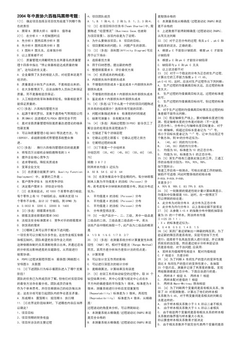
1[1]. 确定项目选择及项目优先级是下列哪个角 色的责任 A. 黑带 B. 黑带大师 C. 绿带 D. 倡导者 2[1]. 在分析 X − R 控制图时应 A. 先分析 X 图然后再分析 R 图 B. 先分析 R 图然后再分析 X 图 C. X 图和 R 图无关,应单独分析 D. 以上答案都不对 3[1]. 质量管理大师戴明先生在其著名的质量管 理十四条中指出“停止依靠检验达成质量的做 法”,这句话的含义是: A. 企业雇佣了太多的检验人员,对经营来说是不 经济的。 B. 质量是设计和生产出来的,不是检验出来的。 C. 在大多数情况下,应该由操作人员自己来保证 质量,而不是靠检验员保证。 D. 人工检验的效率和准确率较低,依靠检验是不 能保证质量的。 4[1](多选).六西格玛管理方法 A. 起源于摩托罗拉,发展于通用电气等跨国公司 B. 其 DMAIC 改进模式与 PDCA 循环完全不同 C. 是对全面质量管理特别是质量改进理论的继承 性新发展 D. 可以和质量管理小组(QCC)等改进方法,与 ISO9001、卓越绩效模式等管理系统整合推 进。 5[1](多选) . 推行六西格玛管理的目的就是要 A. 将每百万出错机会缺陷数降低到 3.4 B. 提升企业核心竞争力 C. 追求零缺陷,降低劣质成本 D. 变革企业文化 6. [2] 在质量功能展开(QFD, Quality Function Deployment) 中,首要的工作是 : A. 客户竞争评估 B. 技术竞争评估 C. 决定客户需求 D. 评估设计特色 7. [2] 在某检验点,对 1000 个某零件进行检验, 每个零件上有 10 个缺陷机会,结果共发现 16 个零件不合格,合计 32 个缺陷,则 DPMO 为 A. 0.0032 B. 3200 C. 32000 D. 1600 8. [2](多选) 顾客需求包括: A. 顾客及潜在顾客的需求(VOC) B. 法规及安全标准需求 C. 竞争对手的顾客需求 D. 供货商的需求 9. [3]哪种工具可以用于解决下述问题: 一项任务可以分解为许多作业,这些作业相互依赖 和相互制约,团队希望把各项作业之间的 这种依赖和制约关系清晰地表示出来,并通过适当 的分析找出影响进度的关键路径,从而能进行 统筹协调。 A. PDPC(过程决策程序图)B. 箭条图(网络图)C. 甘特图 D. 关联图 10. [3]下述团队行为标示着团队进入了哪个发展 阶段? 团队的任务已为其成员所了解,但他们对实现目标 的最佳方法存在着分歧,团队成员仍首先 作为个体来思考,并往往根据自己的经历做出决 定。这些分歧可能引起团队内的争论甚至矛盾。 A. 形成期 B. 震荡期 C. 规范期 D. 执行期 11. [3]在界定阶段结束时,下述哪些内容应当得 以确定? 1、项目目标 2、项目预期的财务收益 3、项目所涉及的主要过程
数据变换的万能钥匙:Box-Cox变换协和八

数据变换的万能钥匙:Box-Cox变换协和八注:本文为协和八「说人话的统计学」系列之《样本分布不正态?数据变换来救场!》的延伸阅读,点击上述标题可跳转至该集原文。
读过两天前推送的《样本分布不正态?数据变换来救场!》,你一定已经熟悉了数据变换的目的和意义,也了解了常用的若干种数据变换函数,如、、等。
至于说什么时候应该用哪个函数来作变换,原文也针对常见的几种情况给出了一些建议。
当然,我们会遇到的数据纷繁复杂,究竟用什么函数效果比较好,还是得通过反复尝试并实际验证才知道。
就好像用单反照相机的手动模式拍照一样,这可是一件需要经验、知识和运气的事儿。
你的内心在呼唤:能不能有自动模式(或者干脆来个傻瓜卡片机)呢?这里我们就来简单介绍一下一种根据数据自动寻找「最佳」变换函数的方法——Box-Cox 变换在上世纪六十年代由两位英国统计学家 George E.P. Box 和 David Cox 提出( Box 他老人家几年前刚刚谢世,而 Cox 现已 92 岁高龄)。
他们两位葫芦里卖的是什么药呢?我们先来看看 Box-Cox 变换的数学形式。
和以前一样,假设样本里一共有 n 个数据点,分别是。
如果我们把变换后新的数据点记为(你会问这个λ是哪里冒出来的?别着急,我们马上解释),那么有:看着很复杂?我们来把它解剖一下,你会发现其实挺简单。
这里出现的λ,是一个有待确定的常数。
这个常数如何确定我们稍等一会再说,现在我们先假设λ的值已经给定了,变换会是个什么样子?把目光投向上述定义的第二行,你会看到一位老熟人——对数变换。
不错,如果λ取 0,那么 Box-Cox 变换让我们做的正是对样本取对数。
如果λ≠0,观察第一行的算式,我们能看到它的核心部分其实就是,后边的-1 和分母的λ只是两个对进行拉伸和平移的常数,并不会影响分布的形状。
是什么呢?不就是个关于y 的幂函数嘛!当λ分别取下列数值时,我们会得到一系列耳熟能详的函数:…你看,我们之前说过的常用的变换函数几乎都出现了!写到这里其实并没有什么神奇的,无非只是利用λ把这些不同的函数写出一个统一的表达式而已。
时间序列 数据清洗和预处理 数据分解 box-cox方法
时间序列数据清洗和预处理数据分解box-cox方法1. 引言1.1 概述:时间序列数据分析是一种广泛应用于各个领域的数据分析方法,它能够揭示时间相关性和趋势,帮助我们预测未来趋势、进行决策和制定策略。
然而,时间序列数据经常存在一些问题,如噪音干扰、缺失值以及非线性等,这些问题会对分析结果的准确性产生负面影响。
因此,在进行时间序列数据分析之前,我们需要进行数据清洗和预处理的工作。
本文将重点讨论时间序列数据清洗和预处理的方法。
1.2 文章结构:本文共分为五个主要部分。
首先,引言部分介绍了文章的概述、目的和重要性。
第二部分将详细介绍时间序列数据清洗和预处理的过程,包括数据收集和获取、数据清理和缺失值处理以及数据平滑和去噪。
第三部分将介绍常用的时间序列数据分解方法,包括经典分解方法和基于小波的分解方法。
第四部分则着重探讨Box-Cox转换方法在时间序列数据预处理中的应用,并提供实现方法和应用案例分析。
最后,在结论与展望部分对本文进行总结并提出改进方向展望。
1.3 目的:本文的目的是探讨时间序列数据清洗和预处理的方法,以及容易忽视但重要的Box-Cox转换方法在时间序列数据分析中的应用。
通过深入了解和研究这些方法,读者将能够更好地理解如何有效地处理时间序列数据,降低噪音干扰、处理缺失值,并提高对数据趋势和相关性的理解能力。
此外,我们还将通过实际案例分析来展示这些方法在实际问题中的应用效果,帮助读者更好地理解其实际价值和应用场景。
最终,我们期望本文对时间序列数据分析领域的从业人员和学术研究者有所帮助,并为进一步研究和应用提供指导。
2. 时间序列数据清洗和预处理2.1 数据收集和获取数据收集是时间序列分析中的第一步,它涉及到获取可用于分析的原始时间序列数据。
常见的数据收集方法包括实时采集、历史数据提取和数据库查询等。
在进行数据收集之前,需要明确所需的时间范围、采样频率以及目标变量等。
2.2 数据清理和缺失值处理在时间序列数据中,经常会遇到许多问题,如异常值(outliers)、噪声(noise)以及缺失值(missing values)等。
BoxCox 变换方法及其实现运用

2
1、 2 ... n
服从 正态分布
应用前提 在处理实际经济问题和社会问题时,由于海量数 据比较凌乱,同时在建立回归模型时,个别变量 的系数通不过。例如生物医学等数据的特殊性, 往往不可观测的误差 可能是和预测变量相关的, 不服从正态分布,于是给线性回归的最小二乘估 计系数的结果带来误差,为了满足上述四个条件 而不丢失信息,有时需要改变一下数据形式,进 而Box-Cox变换得到了广泛推广。
谢 谢!
两种公式对比
当 =0.5时, 当 =0.5
yi
xi
时, y ( ) =2 y 2
=-1 当 时,
1 yi xi
当 =-1时
y ( ) =1 1 y
通过对比Box-Cox特殊变换公式和数据变换公式 ,我们可以发现Box-Cox特殊变换公式就是数据 变换,只是在形式上有一定的改进。
• 倒数转换:
• 平方根后再取反正弦:yi Arc sin( xi ) • 幂转换:y
i
1 xi
xi 1
x
~
1
其中 x ( xi )
i 1
~
n
1/ n
,参数 [1.5,1]
表中数据来自于豪爵摩托车用户满意度问卷调查的样本。通过 大量重复试验,得到如下规律:P值为0.003视为平方转换的一 个界点,如果正态检验得到的p值大于0.003,通过平方转换一 般可实现正态化处理,否则通过平方转换很难实现正态化处理, 其他几种转换方法也往往达不到正态处理的目的。
, 0 变换公式为: y ( ) {log (y) , 0 y 1
逆变换公式为: y {exp( y ( ) ), ,0 0 显然,y的Box-Cox变换是一个变换族,由可变参 数 决定着具体变换的形式,当 0 时,该变换 为对数变换。
基于水平镜像算法的改进Box-Cox变换
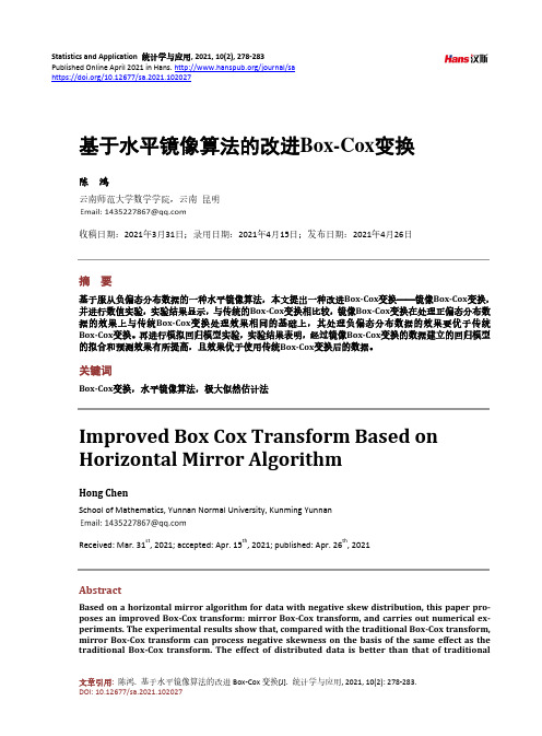
陈鸿
Box-Cox transform. Then the simulated regression model experiment is carried out. The experimental results show that the fitting and prediction effect of the regression model established by the mirror Box-Cox transformation data is improved, and the effect is better than the data after using the traditional Box-Cox transformation.
Open Access
1. 引言
1.1. 研究背景
现实中,我们会遇到的数据纷繁复杂,不同的数据根据我们所做的假设的不同,需要进行不同的变 换,以便我们能够在已有理论上对其进行分析。例如:股票收益率等数据的特殊性,不可观测的误差可 能是和预测变量相关的,但其不服从正态分布,于是给线性回归的最小二乘估计系数的结果带来误差, 为了满足线性回归的四个假设条件而又不丢失信息,有时需要对数据进行处理变换;又例如方差分析需 要试验误差具有独立性、无偏性、方差齐性和正态性的条件,若不满足这些条件就需要对数据进行处理 [1]。
基于水平镜像算法的改进Box-Cox变换
陈鸿 云南师范大学数学学院,云南 昆明
收稿日期:2021年3月31日;录用日期:2021年4月15日;发布日期:2021年4月26日
box-cox变换公式
box-cox变换公式Box-Cox变换是一种常用的数据转换方法,它可以对数据进行幂次变换,从而使数据满足正态分布的假设。
这个方法由两位统计学家,George Box和David Cox在1964年提出,被广泛应用于统计建模和数据分析中。
Box-Cox变换的公式如下:\[y(\lambda)= \begin{cases} \frac{{(y+\lambda)^{\lambda}-1}}{\lambda}, & \text{if } \lambda \neq 0 \\ \ln(y), & \text{if } \lambda = 0 \end{cases}\]其中,y表示原始的数据,y(λ)表示进行Box-Cox变换后的数据,λ是变换的参数。
这个参数可以取任意实数,通过选择不同的λ值,可以得到不同的变换结果。
Box-Cox变换可以用于处理各种类型的数据,包括正数、负数和零。
当λ=0时,变换结果是对数变换,适用于数据中存在负数或零值的情况。
当λ不等于0时,变换结果是幂次变换,可以通过调整λ的值来控制对数据的变换程度。
Box-Cox变换的主要目的是使数据满足正态分布的假设,因为很多统计方法都基于正态分布的假设。
正态分布具有对称性和峰度,而且大部分统计方法在满足正态分布假设时才能得到准确的结果。
因此,通过对数据进行Box-Cox变换,可以消除数据的偏态和尖峰度,使数据更接近于正态分布。
进行Box-Cox变换的步骤如下:1. 选择要进行Box-Cox变换的数据集。
2. 通过绘制数据的直方图或概率图来判断数据的分布情况。
如果数据偏态较大或尖峰度较高,可以考虑进行Box-Cox变换。
3. 选择合适的λ值。
可以通过尝试不同的λ值,并使用统计指标(如最大似然估计)来评估变换后数据的正态性。
一般来说,λ的取值范围在-5到5之间。
4. 根据选择的λ值,计算变换后的数据。
5. 检验变换后的数据是否满足正态分布的假设。
boxcox转换结果的解释 -回复

boxcox转换结果的解释-回复Box-Cox转换是一种用于对数据进行变换的统计方法,可用于处理非正态分布的数据。
它能够通过选择合适的参数lambda(λ)值,将数据转换为更接近正态分布的形式。
本文将详细解释Box-Cox转换的原理和步骤,并深入探讨其在数据分析和建模中的应用。
第一部分:Box-Cox转换的原理Box-Cox转换是由两位统计学家George Box和David Cox于1964年首次提出的。
它基于一个假设,即对数据进行适当的变换可以使其符合正态分布的假设,从而使得统计分析和建模更加准确和可靠。
换句话说,Box-Cox转换的目标是通过一种函数变换,将非正态分布的数据转化为趋近于正态分布的形式。
这可以在某些情况下改善数据分析结果,例如线性回归模型需要满足线性关系、正态分布和等方差性的假设。
通过将数据转换为正态分布,我们可以更好地满足这些假设,从而提高模型的准确性和可解释性。
第二部分:Box-Cox转换的步骤Box-Cox转换的步骤可以概括为以下几个关键步骤:1. 确定数据是否需要进行Box-Cox转换。
这可以通过视觉检查数据的直方图、QQ图和正态性检验来确定。
如果数据明显偏离正态分布,有必要考虑进行Box-Cox转换。
2. 计算数据的Box-Cox转换。
转换公式如下:Y(lambda) = (X^lambda - 1) / lambda其中,X表示原始数据,Y(lambda)表示转换后的数据,lambda是一个可调参数,会根据原始数据的特征进行估计。
对于不同的lambda值,可以得到一系列不同的转换结果。
3. 选择最佳的lambda值。
为了选择最佳的lambda值,可以采用两种常用方法:最大似然估计和交叉验证。
- 最大似然估计(maximum likelihood estimation):通过计算似然函数的最大值来估计最佳的lambda值。
- 交叉验证(cross-validation):将数据分为训练集和验证集,在训练集上估计lambda值,并在验证集上评估模型性能,选取具有最小误差的lambda值。
- 1、下载文档前请自行甄别文档内容的完整性,平台不提供额外的编辑、内容补充、找答案等附加服务。
- 2、"仅部分预览"的文档,不可在线预览部分如存在完整性等问题,可反馈申请退款(可完整预览的文档不适用该条件!)。
- 3、如文档侵犯您的权益,请联系客服反馈,我们会尽快为您处理(人工客服工作时间:9:00-18:30)。
Estimation for Box-Cox Transformation Model With Nonparametric restriction on the error term∗Yahong ZhouSchool of Economics,Shanghai University of Finance and Economics,Shanghai,200433AbstractAs well known,Box-Cox transformation model has been widely used in applied econometrics and statistics.Typically,under the restriction that the error term with normal distribution,estimation and inference procedures for the regression coefficients and transformation parameter under this model setting have been studied extensively.In this paper,we propose a simple semi-parametric estimation method for the Box-Cox transformation model with no specific paprametric assumption on the distribution of the error term.The proposed estimator is consistent and asymptotically normally distributed.Its covariance matrix can be in closed form which can be easily estimated.A small Monte Carlo experiment is done, which demonstrates good performance of our estimator.Keywords:Box-Cox transformation model,Semiparametric estimation,Rank condition,Smoothed kernel. AMS Subject Classification:62G05,62G20.§1IntroductionIn this paper,we consider the estimation of the Box-Cox regression model with a linear structure of the formg(α0,Y i)=X′iβ0+u i(1.1) whereg(α,y)= yα−1∗This paper is a revised version of one chapter of the author’s ph.D.dissertation at the Department of Economics of Hong Kong University of Science and Technology.Thanks to Prof.Songnian Chen for his guidance for this paper as well as seminar participants at HKUST and SHUFE for their valuable comments.Andfinancial support is from research grants no.211-3-50 and no.211-3-70..1For the estimation of the Box-Cox regression model,traditionally,the most common approach is us-ing the maximum likelihood method under the assumption that the error term u is normally distributed. However,as is well known,the normality assumption is not compatible with the transformation model. Furthermore,the error distribution is typically unknown and economic theory provides little guidance on this,any misspecification of the parametric distribution of the error term could lead inconsistency of the es-timates.Instead of making parametric specification for the error distribution,Amemiya and Powell(1981) proposed a nonlinear two-stage least squares(NL2SLS)estimator based on certain moment conditions. However,as pointed out in Foster,Tian and Wei(2000),these moment conditions very often do not pro-vide strong identification conditions,and as a result,the NL2SLS estimator could suffer from some serious finite sample problems due to the existence of possible multiple roots to the sample moment conditions. Amemiya(1985),Newey(1997)and Robinson(1991)proposed asymptotically efficient estimators of the parameters of the Box-Cox transformation model without assuming a parametric structure on the error term.Although their proposals are interesting theoretically,these estimators are often involved in the multiple roots problems in their estimating equations(See,Foster,Tian and Wei(2000)).To relax the parametric assumption on the transformation,Horowitz(1996)considered inference problems for linear regression models with a completely unspecified transformation function.But for this case,regression parameters are not totally identifiable,and also,the nonparametric functional estimate can be quite useful for identifying the shape of the transformation function,which may not be completely convex or concave as for Box-cox parametric transformation.Based on the drawback of the existing literature on this trans-formation model,Foster,Tian and Wei(2000)proposed an estimator for this model,but the covariance matrix of their estimator is too complicated to write down in the closed form,only the bootstrapping can be used to obtain its estimate.In this paper,a relatively simple semiparametric estimation procedure is proposed under the Box-Cox transformation model without assuming parametric form of the disturbance.We show that the resulting estimator is asymptotically normal,unlike Foster Tian and Wei(2000),its covariance matrix is in closed form,which can be easily estimated.This article is organized as follows;in the next section,we propose our rge sample properties for the estimator will be investigated in section3.Section4contains some simulation results from a simple small scale Monte Carlo study.The proofs of large sample properties are given in appendix.§2The EstimatorWhat attracting our interest is the estimation of Box-Cox transformation parameterα0and the slope coefficientsβ0in(1.1).To motivate the estimates ofα0andβ0,we make the following analysis:with strict monotonicity of g,for an observation i,notice thatY i<t⇐⇒g(α0,Y i)<g(α0,t)1(Y i<t)=1(g(α0,Y i)<g(α0,t))=1(X′iβ0+u i<g(α0,t))=1(u i<g(α0,t)−X′iβ0)Analogously,for another observation j,1(Y j<s)=1(u j<g(α0,s)−X′jβ0)2So,for the event of1(Y i<t)given X i,the probability of its taking place is F(g(α0,t)−X′iβ0),where F(.) is the distribution of the error term.For1(Y j<s),the probability of its happening is F(g(α0,s)−X′jβ0). Under the assumption of u i is continuously distributed,the following relationship holds:P(1(Y i<t)|X i,X j)>P(1(Y j<s)|X i,X j)⇐⇒g(α0,t)−X′iβ0>g(α0,s)−X′jβ0For all the observations and possible values of s and t.Based on this rank condition,we propose the estimation ofα0andβ0by maximizing1h1n)can be used to replace the indicator function which has its precedent in Horowitz (1996).Now the estimation ofα0andβ0is given by satisfyingMaxα,β1h1n)dtds(2.2) where the sequences of bandwidth satisfying h1n,as n→∞,further restrictions on the kernel will be given in next section.As we often encounter that the objective function is not necessarily concave.The big problem is that no concavity may result in no unique maximum point.To our objective function in(2.2),it is not an exception,in reality it is hard for us tofigure out which one is the estimate of the true values when more than one extremum points are available,even if not counting difficulty of computation.This implies that directly solving this problem may not be a good approach.Alternatively,with the further analysis below, the problem can be circumvented.Now suppose thatα0were known,Eq.(1.1)becomes a this linear modelg(α0,Y i)=X′iβ0+u iThus,β0can be easily estimated by OLS,denoted asˆβ(α0)=[1n X i g(α0,Y i)](2.3)however,because of unknownα0,estimation ofβ0in(2.3)is infeasible.Now,we defineˆβ(α)byˆβ(α)=[1n X i g(α,Y i)]The above defined functionˆβ(α)describing the relation of the estimatorˆβat any value ofαin its domain. Straightforwardly,we propose to estimateα0byˆα,which maximizes1×K(g(α,t)−X′i ˆβ(α)−(g(α,s)−X′jˆβ(α))nh m11n→0.Assumption1describes the identification conditions which are common in semiparametric estimation. The requirement of the continuous distribution of one of its components is for simplicity,and can be relaxed easily as the way in Chen(2003).Assumption2is a condition on kernel,similar to Horowitz(1996).In assumption3,(1)is both for the consistency and asymptotic normality which is standard in extremum estimator theory;(2)is a sufficient condition for the uniform convergence in the proof of consistency,some parts of them are similar to Robinson(1988).Assumption4is the requirement of Euclidean property for{g(α,Y i),α∈Λ},which is crucial to the uniform law of large number used repeatedly in this section. Assumption5is the restriction for the bandwidths,under this assumption,the bias can be ignored in the asymptotic distribution.Theorem1Under Assumptions1-5,ˆθ=(ˆα,ˆβ(ˆα)′)′is consistent forθ0=(α0,β′0)′.Proof:For the consistency ofˆα,we follow the approach in Amemiya(1985).1)The parameter spaceΛis compact.This is from assumption3;2)Uniform convergence.4DefineS n(α)= 1h1n)dsdt=T n(α,ˆβ(α))=T n(α,β(α))+∂T n(α,¯β(α))n(n−1) i=j(1(Y i<t)−1(Y j<s))×K(g(α,t)−X′iβ(α)−(g(α,s)−X′jβ(α))∂β(ˆβ(α)−β(α))can be expressed as∂T n(α,¯β(α))n(n−1) i=j(1(Y i<t)−1(Y j<s))k(g(α,t)−X′i¯β(α)−(g(α,s)−X′j¯β(α))h1ndsdt×(ˆβ(α)−β(α))where k(.)is the derivative of K(.),as assumed to be bounded and k(t)dt=1in assumption2.β(α)will be defined below.First recallˆβ(α)=[1n X i g(α,Y i)]β(α)is defined as the limit form ofˆβ(α).by the assumption3.It is straightforward to show that[1n X i g(α,Y i)→p E[X i g(α,Y i)]uniformly inα.Now,β(α)can be written asβ(α)=[E(X i X′i)]−1E[X i g(α,Y i)]5considering the fact that Box-Cox transformation g(α,Y)can keep the property of Euclidean as pointed out by Joslin and Sherman(2002),so the summation termX i g(α,Y i),α∈Λ}is Euclidean for some envelope F with P F2<+∞under assumption3.So we have1n)it follows immediately that|ˆβ(α)−β(α)|=O p(1n)(3.2)supα∈Λfrom the expression ofβ(α),we haveβ(α0)=β0.We return to(3.1),in which the second term is ignored by(3.2).For thefirst term1)dsdth1nagain,g(α,t)is the Box-Cox transformation,for any given s,t,1(Y i<t),1(Y j<s),are indicator functions, K(.)are the functions of bounded variation,andg(α,t)−X′iβ(α)−(g(α,s)−X′jβ(α)))h1nAs h1n→0,with the dominated convergence theory,the limitation of which isE[(F(g(α0,t)−X′iβ0)−F(g(α0,s)−X′jβ0))×1(g(α,t)−X′iβ(α)>g(α,s)−X′jβ(α))]dsdt(3.3) Thus,define S(α)S(α)= E[(F(g(α0,t)−X′iβ0)−F(g(α0,s)−X′jβ0))×1(g(α,t)−X′iβ(α)>g(α,s)−X′jβ(α))]dsdtFor this S(α),which is the limitation of S n(α)satisfyingS n(α)−ES n(α)=o p(1)uniformly inαUsing the property of Euclidean.ES n(α)−S(α)=o p(1)uniformly inα6with bounded convergence theory.It is obvious that|S n(α)−S(α)|→p0.(3.4)supα∈Λ3)Next we prove thatα0uniquely maximizes S(α);First,α0maximizes S(α);From the expression of S(α),ifα=α0,note thatβ(α0)=β0,based on the rank condition,it is obvious thatα=α0maximizes S(α).The uniqueness ofα0;Suppose that there exists˜α=α0,andβ(˜α)maximize S(α),S(˜α)can be writtenS(˜α)= E[(F(g(α0,t)−X′iβ0)−F(g(α0,s)−X′jβ0))×1(g(˜α,t)−X′iβ(˜α)>g(˜α,s)−X′jβ(˜α))]dsdtdefineG(α0,β0,X i,X j,t,s)=g(α0,t)−X′iβ0−(g(α0,s)−X′jβ0)for any given X0i and X0j in domain,we can easilyfind some t0,s0such thatG(α0,β0,X0i,X0j,t0,s0)=0Using X′iβ,X′jβare continuously distributed,and from assumption4,G(˜α,β(˜α),X0i,X0j,t0,s0)=g(˜α,t0)−X′iβ(˜α)−(g(˜α,s0)−X′jβ(˜α))=0without loss generality,suppose G(˜α,β(˜α),X0i,X0j,t0,s0)>0,from G(α0,β0,X0i,X0j,t0,s0)=0,in the neighborhood of(X0i,X0j,t0,s0),we canfind a subset B in which,G(α0,β0,X i,X j,t,s)<0,but G(˜α,β(˜α),X i,X j,t,s)>0SoS(˜α)<S(α0)This contradicts the assumption above,which implies that the uniqueness ofα0.4)S(α)is continuous.From the expression of S(α),it follows immediately.Now,by1)-4),the consistency ofˆαis straightforward.After proving the consistency ofˆα,we turn to the estimation ofβ0(the slope parameters).Intuitively, since we have shown thatˆαis the consistent estimator ofα0,as mentioned in last section,ˆβ(ˆα)is a candidate estimator ofβ0.Actually its consistency can be argued as follows:ˆβ(ˆα)−β=(ˆβ(ˆα)−β(ˆα))+(β(ˆα)−β0)In which,on the right hand side thefirst termˆβ(ˆα)−β(ˆα)→p0by the uniform convergence ofˆβ(α)→p β(α)for anyαinΛ,as shown in the proof of consistency ofˆα.The second termβ(ˆα)−β0=β(ˆα)−β(α0)from the expression ofβ(α),obviously,it is continuous in the neighborhood ofα0.Then|β(ˆα)−β(α0)|→p0 asˆαis the consistent estimator ofα0.Soˆβ(ˆα)→β0(3.5)p7After the proof of the consistency ofˆαandˆβ(ˆα),we turn to investigate the asymptotic normality of our estimator.For notation simplicity,denoteQ11(t,s,X′iβ0,X′jβ0)=E[(g′(α0,t)−X′iβ′(α0)−(g′(α0,s)−X′jβ′(α0)))2|X′iβ0,X′jβ0]whereβ′(α0)is the derivative ofβ(α)evaluated atα=α0.Q12(t,s,X′iβ0,X′jβ0)=E[g′′(α0,t)−X′iβ′′(α0)−(g′′(α0,s)−X′jβ′′(α0))|X′iβ0,X′jβ0]whereβ′′(α0)is the second derivative ofβ(α)evaluated atα=α0.Q13(X′jβ0)=E[X′jβ′(α0))|X′jβ0]Q14(s,t,X′iβ0,X′jβ0)=E[(g′(α0,t)−X′iβ′(α0)−(g′(α0,s)−X′jβ′(α0)))×(−X′i+X′j)|X′iβ0,X′jβ0]Q15(s,t,X′iβ0,X′jβ0)=Q14(s,t,X′iβ0,X′jβ0)f X′j β0 (X′jβ0)Q16(X′jβ0)=E(X′j|X′jβ0)M1= E[f u(g(α0,t)−X′iβ0)×Q11(t,s,X′iβ0,g(α0,s)−g(α0,t)+X′iβ0)×f X′β0(g(α0,s)−g(α0,t)+X′iβ0)]dsdtM2= E[f u(g(α0,t)−X′iβ0)×Q15(s,t,X′iβ0,g(α0,s)+X′iβ0−g(α0,t))]dsdtΦi=[EX i X′i]−1X i u iΨi= (1(Y i<t)−F(g(α0,t)−X′iβ0))×(g′(α0,t)−X′iβ′(α0)−g′(α0,s)+Q13(g(α0,s)−g(α0,t)+X′iβ0)×f X′β0(g(α0,s)−g(α0,t)+X′iβ0)dsdtTheorem2Under Assumptions1-5,ˆθ=(ˆα,ˆβ(ˆα)′)′is asymptotically normally distributed satisfying,√√n(ˆβ(ˆα)−β0)=1n U i+o p(1) 8and√n(ˆβ(ˆα)−β0)d→N(0,EU i U′i)where V i=M−11(2Ψi+M2Φi)and U i=β′(α0)M−11(2Ψi+M2Φi)+Φi,β′(α0)is the derivative ofβ(α) evaluated atα=α0.The proof of asymptotic normality will be given in the appendix;To carry out statistical inference,we need to estimate the asymptotic covariance matrix ofˆαand ˆβ(ˆα),which can be constructed,but in complicated forms.Here we only briefly discuss the estimation of the variance ofˆαandˆβ(ˆα).From the functions defined above,Q11could be estimated nonparametrically, the true valuesα0,β0andβ′(α0)can be replaced by their corresponding estimators,it follows thatˆQ11=ˆQ11(t,s,X′iˆβ0,X′jˆβ0)(3.6) so M1can be estimated by replacing the density of X′β0,the error term’s density by nonparametric density estimation of X′ˆβ(ˆα),X′ˆβ(ˆα)and the expectation in Q11is approximated by sample mean with the law of large number,Now defineˆM 1=1n(ˆα−α0)can be estimatedˆV 1=1n(ˆβ(ˆα)−β0)can be estimated byˆV 2=1nni=1||ˆΨi−Ψi||2=o p(1)1nni=1||ˆM−11(2ˆΨi+ˆM2ˆΦi)−M−11(2Ψi+M2Φi)||2=o p(1)Consequently,the consistency ofˆV1follows.So does the consistency ofˆV2.9§4A Monte Carlo StudyIn this section,a small Monte Carlo experiment is presented to test thefinite sample performance and illustrate the usefulness of our estimator.We will report the Mean,Bias,SD(standard deviation) and RMSE(the root of mean squared error)of estimates ofα0andβ0.All these designs are based on 100replications for each design with sample size n=100.The simulation is composed of following three designs.For the data generating simplicity,a generalized Box-Cox transformation is adopted in all designs, which has the form g(λ,Y i)=|Y|λsign(Y)−1True value Bias RMSE0.3-0.02560.108010.03920.09760.50.00200.05221-0.00210.08370.70.00460.08701-0.00240.06701-0.03660.068010.01290.0766The main difference in these designs is the different selection of true value ofα.The objective of this simulation is to test its performance at different level of the transformation parameter.From the listed values of the above table,no matter what the true value forα0is0.3,0.5,0.7or1,we have seen that our estimator performs stably and satisfactorily under not large enough sample size(in all four designs,the sample size n=200),and we also can see the goodfitness of the estimate ofβ0in all four designs.AppendixThe proof of asymptotic normality;10Recall thatˆαmaximizes the objective function1h1n)dtds F.O.C with respect toα,it follows that1h1n)×g′(ˆα,t)−X′i ˆβ′(ˆα)−(g′(ˆα,s)−X′jˆβ′(ˆα))n(n−1) i=j(1(Y i<t)−1(Y j<s))×k(g(ˆα,t)−X′i ˆβ(ˆα)−(g(ˆα,s)−X′jˆβ(ˆα))h1ndsdtTaylor expansion for G(ˆα,ˆβ(ˆα),ˆβ′(ˆα))=0with respect toαatα0,G(ˆα,ˆβ(ˆα),ˆβ′(ˆα))=G(α0,ˆβ(α0),ˆβ′(α0))+dG(¯α,ˆβ(¯α),ˆβ′(¯α))dα√nG(α,ˆβ(α0),ˆβ′(α0))(A.1’)where¯αlies on the segment ofα0andˆα,anddG(α,ˆβ(α),ˆβ′(α))n(n−1)[ i=j(1(Y i<t)−1(Y j<s))[k′(g(α,t)−X′iˆβ(α)−(g(α,s)−X′jˆβ(α))h1n)2+k(g(α,t)−X′iˆβ(α)−(g(α,s)−X′jˆβ(α))h1n]dsdt11Recall thatˆβ(α)=β(α)+O p(1n)uniformly inα,from the definition ofˆβ(α),it involves the Box-Cox transformation function.Following the way of Joslin and Sherman(2002)which deals with the nonlinear function of V C class,what needed to process isˆβ′(α)andˆβ′′(α),forˆβ′(α)ˆβ′(α)=[1n X i g′(α,Y i)]it is easily seen that for any given yg′(α,y)=αyαln y−(yα−1)√√dα=dG(α,β(α),β′(α))dα=dG(¯α,β(¯α),β′(¯α))dα=1h1n)×(g′(¯α,t)−X′iβ′(¯α)−(g′(¯α,s)−X′jβ′(¯α))h1n)×g′′(¯α,t)−X′iβ′′(¯α)−(g′′(¯α,s)−X′jβ′′(¯α))dα→p E[dG(α,β(α),β′(α))dα|α=α0+o p(1)]→p E[dG(α0,β(α0),β′(α0))dG(α0,β(α0),β′(α0))E[)h1n×(g′(α0,t)−X′iβ′(α0)−(g′(α0,s)−X′jβ′(α0)))h1n×g′′(α0,t)−X′iβ′′(α0)−(g′′(α0,s)−X′jβ′′(α0))=ω1h1ng(α0,s)−X′jβ0=g(α0,t)−X′iβ0−h1nω1plug in(A.3)E{ (F(g(α0,t)−X′iβ0)−F(g(α0,t)−X′iβ0−h1nω1))1[k2(ω1)Q12(t,s,X′iβ0,g(α0,s)−g(α0,t)+X′iβ0+h nω1)]h1n×h1n f X′β(g(α0,s)−g(α0,t)+X′iβ0+h nω1)dω1}dsdt→M1= E[f u(g(α0,t)−X′iβ0)×Q11(t,s,W i,X′iβ0,W i,g(α0,s)−g(α0,t)+X′iβ0)×f X′jβ0(g(α0,s)−g(α0,t)+X′iβ0)]dsdt13Where f u(.)is the density of the error term.So thefirst order condition(A.1’)can be written as−(M1+o p(1))√nG(α0,β(α0),β′(α0))+∂Gn(ˆβ(α0)−β(α0))+∂Gn(ˆβ′(α0)−β′(α0))A.4(7)where¯βis betweenˆβ(α0)andβ0(β(α0)=β0),while˘βis betweenˆβ′(α0)andβ′(α0).Let’s discuss(A.4)term by term.For G(α0,β(α0),β′(α0)),with the same argument with that in the proof of consistency,its expectationEG(α0,β(α0),β′(α0))= E{(1(Y i<t)−1(Y j<s))×k2(g(α0,t)−X′iβ0−(g(α0,s)−X′jβ0)h1n}dsdt= E{(F(g(α0,t)−X′iβ0)−F(g(α0,s)−X′jβ0))×k(g(α0,t)−X′iβ0−(g(α0,s)−X′jβ0)h1n}dsdtdenoteQ13(X′jβ0)=E[X′jβ′(α0))|X′jβ0]The expectation of G(α0,β(α0),β′(α0))can be writtenEG(α0,β(α0),β′(α0))= {E(F(g(α0,t)−X′iβ0)−F(g(α0,s)−X′jβ0))×k(g(α0,t)−X′iβ0−(g(α0,s)−X′jβ0)h1n[g′(α0,t)−Q13(X′iβ0)−g′(α0,s)+Q13(X′jβ0)]dsdt= {E(F(g(α0,t)−X′iβ0)−F(g(α0,t)−X′iβ0−h1nω))×k(ω)[g′(α0,t)−Q13(X′iβ0)−g′(α0,s)+Q13(X′iβ0+g(α0,s)−g(α0,t)+h1tω)f X′β(X′iβ0+g(α0,s)−g(α0,t)+h1tω)dsdtwhere we assume that k(.)is m1−order kernel.After Taylor expansion of h1nω.It followsEG(α0,β(α0),β′(α0))=O(h m11n)14denote Z i =(Y i ,X i ),for given s and t,the integrand in G (α0,β(α0),β′(α0))is a U −Statistic ,define A 1as A 1=(1(Y i <t )−1(Y j <s ))×k (g (α0,t )−X ′i β0−(g (α0,s )−X ′j β0)h 1ndsdtUsing the projection theory of U −Statistic.G (α0,β(α0),β′(α0))=E A 1+1n(P A 1(.,Z i ,α0)−E A 1)+S 2n h 1where P is the projection operator,h 1=A 1−P A 1(Z i ,.,α0)−P A 1(.,Z i ,α0),S 2n is the degenerated secondorder U −Statistic .Actually S 2n h 11=o p (1nh m 11n →0,it is straightforwardthat √nG (α0,β(α0),β′(α0))has the same distribution with1n n i =1P A 1(Z i ,.,α0)+1n ni =1P A 1(.,Z i ,α0)Now,denote E j (.)be the expectation with respect to variable X ′j β0.We concentrate on1n n i =1P A 1(Z i ,.,α0)=1n ni =1E j (E (A 1(Z i ,.,α0)|X ′j β0))=1n ni =1E j (1(Y i <t )−F (g (α0,s )−X ′j β0))×1h 1n)×(g ′(α0,t )−X ′i β′(α0)−g ′(α0,s )+Q 13(X ′j β0))dsdt=1n ni =1 [(1(Y i <t )−F (g (α0,s )−X ′j β0))×1h 1n)(g ′(α0,t )−X ′i β′(α0)−g ′(α0,s )+Q 13(X ′j β0))f Xβ(X ′j β0)d (X ′j β0)]dsdt=1n ni =1[(1(Y i <t )−F (g (α0,t )−X ′i β0−h 1n ω))×k (ω)(g ′(α0,t )−X ′i β′(α0)−g ′(α0,s )+Q 13(g (α0,s )−g (α0,t )+X ′i β0+h 1n ω)f Xβ(g (α0,s )−g (α0,t )+X ′i β0+h 1n ω)]dωdsdt15=1n ni =1(1(Y i <t )−F (g (α0,s )−X ′i β0))×(g ′(α0,t )−X ′i β′(α0)−g ′(α0,s )+Q 13(W i ,g (α0,s )−g (α0,t )+X ′i β0)×f Xβ(g (α0,s )−g (α0,t )+X ′i β0)dsdt +√√√√nO (h m 11n )A.6(9)From (A.6)and (A.5),actually they are the same.So define Ψi to beΨi=(1(Y i <t )−F (g (α0,t )−X ′i β0))×(g ′(α0,t )−X ′i β′(α0)−g ′(α0,s )+Q 13(g (α0,s )−g (α0,t )+X ′i β0)f Xβ(g (α0,s )−g (α0,t )+X ′i β0)dsdt√√∂β|β=¯β,β′=˘β√n (n −1)i =j(1(Y i <t )−1(Y j <s ))×k ′(g (α0,t )−X ′i ¯β−(g (α0,s )−X ′j ¯β)h 1n−X ′i +X ′jn (ˆβ(α0)−β0)For the part in the bracket,with the continuity of k ′and the fact that ¯βis between β0and ˆβ,and ˘βlies on the segment of ˆβ′(α0)and β′(α0),Using the U −statistic theory again,which converges toE [(1(Y i <t )−1(Y j <s ))k ′(g (α0,t )−X ′i β−(g (α0,s )−X ′j β)h 1n−X ′i +X ′j= E[(1(Y i<t)−1(Y j<s))k′(g(α0,t)−X′iβ−(g(α0,s)−X′jβ)h1n−X′i+X′jh1n) g′(α0,t)−X′iβ′(α0)−(g′(α0,s)−X′jβ′(α0))h1n]dsdt+o p(1) so it will lead to= E[(F(g(α0,t)−X′iβ0)−F(g(α0,s)−X′jβ0))×k′(g(α0,t)−X′iβ0−(g(α0,s)−X′jβ0)h1n−X′i+X′jh21n k′(g(α0,t)−X′iβ0−(g(α0,s)−X′jβ0)h1nk′2(ω)Q14(s,t,X′iβ0,g(α0,s)−g(α0,t)+X′iβ0+h1nω)×f X′β0(g(α0,s)−g(α0,t)+X′iβ0+h1nω)]dωdsdt For the notation simplicity,define Q15as following:Q15(s,t,X′iβ0,X′jβ0)=Q14(s,t,X′iβ0,X′jβ0)×f X′j β0 (X′jβ0)]whereQ14(s,t,X′iβ0,X′jβ0)=E(g′(α0,t)−X′iβ′(α0)−(g′(α0,s)−X′jβ′(α0))(−X′i+X′j))|X′iβ0,X′jβ0) so the term in the bracket becomes= E [(F(g(α0,t)−X′iβ0)−F(g(α0,t)−X′iβ0−h1nω1))×1+f u(g(α0,t)−X′iβ0−h1nω1)×Q15(s,t,X′iβ0,g(α0,s)+X′iβ0−g(α0,t)+h2nω1)k(ω1)]dω1dsdt→M2= E(f u(g(α0,t)−X′iβ0)×Q15(s,t,X′iβ0,g(α0,s)+X′iβ0−g(α0,t))dsdtas h1n→0.The second term can be expressed asA2=M2×√n(ˆβ(α0)−β0)=1n Φi+o p(1)whereΦi=[EX i X′i]−1X i u i Next we will focus on the third termA3=∂Gn(ˆβ′(α0)−β′(α0))=1h1n)−X′i+X′j n(ˆβ′(α)−β′(α0))dsdt The same approach to the second term above,A3= E[(1(Y i<t)−1(Y j<s))×k(g(α0,t)−X′iβ0−(g(α0,s)−X′jβ0)h1n ]dsdt×√h1n)−X′i+X′jh1nk(g(α0,t)−X′iβ0−(g(α0,s)−X′jβ0)=E (F(g(α0,t)−X′iβ0)−F(g(α0,t)−X′iβ0−h1nω))×(−X′i+Q16(g(α0,s)+X′iβ0−g(α0,t)+h1nω))k(ω)dωwhere Q16(X′jβ0)=E(X′j|X′jβ0).With the result that√n(ˆα−α0)=2n Ψi+M2(1n Φi)+o p(1)=1n V i+o p(1)√n[ˆβ(α0)−β0]=1n Φi+o p(1)For thefirst term,in whichˆβ′(˜α)→pβ′(α0).(based onˆβ′(α)→pβ′(α)uniformly inα,and the continuity ofβ′(α)),so√n(ˆβ(ˆα)−β0)=β′(α0)√√√√n(ˆβ(ˆα)−β0)→N(0,EU i U′i).where U i=β′(α0)M−11(2Ψi+M2Φi)+Φi.19References[1]Amemiya,T.(1985).Advanced Econometrics,Harvard University Press,Cambridge.[2]Box,G.E.P.and D.R.Cox(1964),“An Analysis of Transformations,”Journal of the Royal Statistical Society,Series B.,26,211-252.[3]Chen,S.(2003):“Distribution-free Estimation of the Box-Cox Regression Model With Censoring,”manuscripts.[4]Foster,A,Tian,T.and Wei,L.J.(2000):“Estimation for Box-Cox Transformation Model without assumingparametric error distribution,”Forthcoming in the Journal of American Statistical Association.[5]Horowitz,J.L.(1996):“Semiparametric Estimation of a Regression Model with an Unknown Transformationof the Dependent Variable,”64,103-137.[6]Horowitz,J.L.(1998):Semiparametric Methods in Econometrics,Springer.[7]Hulten,C.R.and F.C.Wykoff(1981):“The estimation of economic depreciation using vintage asset prices,”Journal of Econometrics,15,367-396.[8]Joslin,S.and R.P.Sherman(2002):“An Equivalence Result for VC Classes of Sets”Manuscript.[9]Newey,W.K.(1997):“Convergence rates and Asymptotic Normality for Series Estimators,”Journal of Econo-metrics79,147-168.[10]Pakes,A.and D.Pollard:“Simulation and The Asymptotics of Optimization Estimation,”Econometrica,57,1027-1057.[11]Powell,J.L.,J.H.Stocker and T.M.Stoker(1989):“Semiparametric Estimation of Weighted Average Deriva-tives,”Econometrica,57,1403-1430.[12]Robinson,P.(1988):“Root-n-consistent Semeparametric Regression,”Econometrica,56,931-954.[13]Robinson,P.(1991):“Best Nonlinear Three-Stage Least Squares Estimation of Certain Econometric Models,”Econometrica,59,755-786.[14]Ruud,P.(2000):An Introduction to Classical Econometric Theory,Oxford University Press.Box-Cox(200433)Box-CoxBox-CoxBox-CoxO212.420。