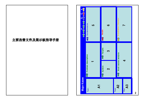
Topic 3 SRM 1

14
SIMPLE REGRESSION MODEL
Y
P4
P1
P2 P3
X1
X2
X3
X4
X
In practice we can see only the P points.
15
SIMPLE REGRESSION MODEL
Y
P4
ˆ Y b1 b 2 X
P1
P2 P3
b1
X1
X2
X3
X4
X
Obviously, we can use the P points to draw a line which is an approximation to the line Y = b1 + b2X +u. If we write this line Y = b1 + b2X, b1 is an estimate of b1 and b2 is an estimate of b2.
16
SIMPLE REGRESSION MODEL
Y (actual value) Y
ˆ Y
(fitted value) R3
P4
ˆ Y b1 b 2 X
P1
R1 b1
R2 P3
R4
P2
X1
X2
X3
X4
X
The line is called the fitted model or sample regression model and the values of Y predicted by it are called the fitted values of Y. They are given by the heights of the R points.
2
The modern interpretation of REGRESSION: Regression analysis is concerned with the study of the dependence of one variable, the dependent variable, on one or more other variables, the explanatory variables, with a view to estimating and/or predicting the (population) mean or average value of the former in terms of the known or fixed (in repeated sampling) values of the latter.
17
SIMPLE REGRESSION MODEL
Y (actual value) Y
ˆ Y
(fitted value) (residual) R3 e1 P1 R1 R2 e2 P2 P3 e3 e4
P4
ˆ Y b1 b 2 X
ˆ Y Y e
R4
b1
X1
X2
X3
X4
X
The discrepancies between the actual and fitted values of Y are known as the residuals, e.
10
1.
2.
3.

5. 6.
SIMPLE REGRESSION MODEL

Some Basic Assumptions on u in SRM

The expected value of u, the disturbance term, in the population is 0. That is,
Y = b 1 + b 2X .
6
SIMPLE REGRESSION MODEL
Y
Y b1 b2X
b1
Q1
Q2
Q3
Q4
X1
X2
X3
X4
X
If the relationship were an exact one, the observations would lie on a straight line and we would have no trouble obtaining accurate estimates of b1 and b2.
8
SIMPLE REGRESSION MODEL
Y
P4
Y b1 b2X
P1
b1
Q1
Q2 P2
Q3 P3
Q4
X1
X2
X3
X4
X
To allow for such divergences, we will write the model as Y = b1 + b2X + u, where u is a disturbance term. A disturbance term is the deviation of an individual Yi around its expected value. It is an unobservabable random variable taking positive or negative values.
Q4
b1
b1 b2X 1
X1
X2
X3
X4
X
Each value of Y thus has a non-random component, b1 + b2X, and a random component, u. The first observation has been decomposed into these two components.
Topic 3. SIMPLE REGRESSION MODEL
（1）

SIMPLE REGRESSION MODEL (简单回归模型 ) LEAST SQUARES REGRESSION (最小二乘法 )

1
Historical origin of the term “Regression”:
This term was introduced by Francis Galton (1886). In a famous paper, Galton found that, although there was a tendency for tall parents to have tall children and for short parents to have short children, the average height of children born of parents of a given height tended to move or “regress” toward the average height in the population as a whole. In other words, the average height of sons of a group of tall fathers was less than their fathers’ height and the average height of sons of a groups of short fathers was greater than their fathers’ height.
E (u) = 0
This assumption means that the factors subsumed in ui do not systematically affect the mean value of Y; so to speak, the positive ui values cancel out the negative ui values so that their average or mean affect on Y is zero.
-1.000
SIMPLE REGRESSION MODEL
Y
Y b1 b2X
b1
X1
X2
X3
X4
X
Suppose that a variable Y is a linear function of another variable X, with unknown parameters b1 and b2 that we wish to estimate. Therefore, as a first approximation, we may write the function as
7
SIMPLE REGRESSION MODEL
Y
P4
Y b1 b2X
P1
b1
Q1
Q2 P2
Q3 P3
Q4
X1
X2
X3
X4
X
In practice, most economic relationships are not exact and the actual values of Y are different from those corresponding to the straight line.
X = independent variable, exogenous variable or regressor Y = dependent or endogenous variable b1 = intercept b2 = slope ui = disturbance term
12
SIMPLE REGRESSION MODEL
18
SIMPLE REGRESSION MODEL
Y (actual value) Y
ˆ Y