数学专业外文文献翻译
数学专业外文文献翻译

第3章 最小均方算法3.1 引言最小均方(LMS ,least-mean-square)算法是一种搜索算法,它通过对目标函数进行适当的调整[1]—[2],简化了对梯度向量的计算。
由于其计算简单性,LMS 算法和其他与之相关的算法已经广泛应用于白适应滤波的各种应用中[3]-[7]。
为了确定保证稳定性的收敛因子范围,本章考察了LMS 算法的收敛特征。
研究表明,LMS 算法的收敛速度依赖于输入信号相关矩阵的特征值扩展[2]—[6]。
在本章中,讨论了LMS 算法的几个特性,包括在乎稳和非平稳环境下的失调[2]—[9]和跟踪性能[10]-[12]。
本章通过大量仿真举例对分析结果进行了证实。
在附录B 的B .1节中,通过对LMS 算法中的有限字长效应进行分析,对本章内容做了补充。
LMS 算法是自适应滤波理论中应用最广泛的算法,这有多方面的原因。
LMS 算法的主要特征包括低计算复杂度、在乎稳环境中的收敛性、其均值无俯地收敛到维纳解以及利用有限精度算法实现时的稳定特性等。
3.2 LMS 算法在第2章中,我们利用线性组合器实现自适应滤波器,并导出了其参数的最优解,这对应于多个输入信号的情形。
该解导致在估计参考信号以d()k 时的最小均方误差。
最优(维纳)解由下式给出:10w R p-= (3.1)其中,R=E[()x ()]Tx k k 且p=E[d()x()] k k ,假设d()k 和x()k 联合广义平稳过程。
如果可以得到矩阵R 和向量p 的较好估计,分别记为()R k ∧和()p k ∧,则可以利用如下最陡下降算法搜索式(3.1)的维纳解:w(+1)=w()-g ()w k k k μ∧w()(()()w())k p k R k k μ∧∧=-+2 (3.2) 其中,k =0,1,2,…,g ()w k ∧表示目标函数相对于滤波器系数的梯度向量估计值。
一种可能的解是通过利用R 和p 的瞬时估计值来估计梯度向量,即 ()x()x ()TR k k k ∧=()()x()p k d k k ∧= (3.3) 得到的梯度估计值为()2()x()2x()x ()()T w g k d k k k k w k ∧=-+2x()(()x ()())Tk d k k w k =-+ 2()x()e k k =- (3.4)注意,如果目标函数用瞬时平方误差2()e k 而不是MSE 代替,则上面的梯度估计值代表了真实梯度向量,因为2010()()()()2()2()2()()()()Te k e k e k e k e k e k e k w w k w k w k ⎡⎤∂∂∂∂=⎢⎥∂∂∂∂⎣⎦2()x()e k k =-()w g k ∧= (3.5)由于得到的梯度算法使平方误差的均值最小化.因此它被称为LMS 算法,其更新方程为 (1)()2()x()w k w k e k k μ+=+ (3.6) 其中,收敛因子μ应该在一个范围内取值,以保证收敛性。
数学专业英语论文(含中文版)
Some Properties of Solutions of Periodic Second OrderLinear Differential Equations1. Introduction and main resultsIn this paper , we shall assume that the reader is familiar with the fundamental results and the stardard notations of the Nevanlinna’s value distribution theory of meromorphic functions [12, 14, 16]。
In addition , we will use the notation )(f σ,)(f μand )(f λto denote respectively the order of growth , the lower order of growth and the exponent of convergence of the zeros of a meromorphic function f ,)(f e σ([see 8]),the e —type order of f(z), is defined to ber f r T f r e ),(log lim)(+∞→=σ Similarly , )(f e λ,the e —type exponent of convergence of the zeros of meromorphic functionf , is defined to be rf r N f r e )/1,(log lim )(++∞→=λ We say that )(z f has regular order of growth if a meromorphic function )(z f satisfiesrf r T f r log ),(log lim )(+∞→=σ We consider the second order linear differential equation0=+''Af fWhere )()(z e B z A α=is a periodic entire function with period απω/2i =。
数学专业毕业设计文献翻译

附件1:外文资料翻译译文第1章预备知识双曲守恒律系统是应用在出现在交通流,弹性理论,气体动力学,流体动力学等等的各种各样的物理现象的非常重要的数学模型。
一般来说,古典解非线性双曲方程柯西问题解的守恒定律仅仅适时局部存在于初始数据是微小和平滑的.这意味着震波在解决方案里相配的大量时间里出现。
既然解是间断的而且不满足给定的传统偏微分方程式,我们不得不去研究广义的解决方法,或者是满足分布意义的方程式的函数.我们考虑到如下形式的拟线性系统, (1.0.1)这里是代表物理量密度的未知矢量向量,是给定表示保守项的适量函数,这些方程式通常被叫做守恒律.让我们假设一下,是(1.0.1)在初始数据. (1.0.2)下的传统解。
使成为消失在紧凑子集外的函数的一类。
我们用乘以(1.0.1)并且使的部分,得到. (1.0.3)定义1.0.1 有,,有界函数叫做在以原始数据为边界条件下,(1.0.1)初值问题的一个弱解,在(1.0.3)适用于所有.非线性系统守恒理论的一个重要方面是这些方程解的存在疑问性.它正确的帮助解答在手边的已经建立的自然现象的模型的问题,而且如果在问题是适定的.为了得到一个总体的弱解或者一个考虑到双曲守恒律的普遍的解,一个为了在(1.0.1)右手边增加一个微小抛物摄动限:(1.0.4)在这是恒定的.我们首先应该得到一个关于柯西问题(1.0.4),(1.0.2)对于任何一个依据下列抛物方程的一般理论存在的的解的序列:定理1.0.2 (1)对于任意存在的, (1.0.4)的柯西问题在有界可测原始数据(1.0.2)对于无限小的总有一个局部光滑解,仅依赖于以原始数据的.(2)如果解有一个推理的估量对于任意的,于是解在上存在.(3)解满足:如果.( 4)特别的,如果在(1.0.4)系统中的一个解以(1.0.5)形式存在,这里是在上连续函数,,如果(1.0.6) 这里是一个正的恒量,而且当变量趋向无穷大或者趋向于0时,趋向于0.证明.在(1)中的局部存在的结果能简单的通过把收缩映射原则应用到解的积分表现得到,根据半线性抛物系统标准理论.每当我们有一个先验的局部解的评估,明显的本地变量一步一步扩展到,因为逐步变量依据基准.取得局部解的过程清晰地表现在(3)中的解的行为.定理1.0.2的(1)-(3)证明的细节在[LSU,Sm]看到.接下来是Bereux和Sainsaulieu未发表的证明(cf. [Lu9, Pe])我们改写方程式(1.0.5)如下:(1.0.7)当.然后. (1.0.8) 以初值(1.0.8)的解能被格林函数描写:. (1.0.9)由于,,(1.0.9)转化为.(1.0.10)因此对于任意一个,有一个正的下界.在定理1.0.2中获得的解叫做粘性解.然后我们有了粘性解的序列,,如果我们再假如是在关于参数的空间上一致连续,即存在子序列(仍被标记)如下, 在上弱对应(1.0.11) 而且有子序列如下,弱对应(1.0.12) 在习惯于成长适当成长性.如果,a.e.,(1.0.13)然后明显的是(1.01)使在(1.0.4)的趋近于0的一个初始值(1.0.2)的一个弱解.我们如何得到弱连续(1.0.13)的关于粘度解的序列的非线性通量函数?补偿密实度原理就回答了这个问题.为什么这个理论叫补偿密实度?粗略的讲,这个术语源自于下列结果:如果一个函数序列满足(1.0.14)与下列之一或者(1.0.15) 当趋近于0时弱相关,总之,不紧密.然而,明显的,任何一个在(1.0.15)中的弱紧密度能补偿使其成为的紧密度.事实上,如果我们将其相加,得到(1.0.16)当趋近于0时弱相关,与(1.0.14)结合意味着的紧密度.在这本书里,我们的目标是介绍一些补偿紧密度方法对标量守恒律的应用,和一些特殊的两到三个方程式系统.此外,一些具有松弛扰动参量的物理系统也被考虑进来。
数学专业英语第三版课文翻译章

数学专业英语第三版课文翻译章本文将根据数学专业英语第三版课文《Step by Step Thinking》进行翻译。
"Step by Step Thinking"is an article that introduces the concept of step-by-step thinking in mathematics.It highlights the importance of breaking down complex problems into smaller,more manageable steps in order to solve them effectively.The article begins by stating that step-by-step thinking is a fundamental skill in mathematics.It emphasizes the need to approach problems by breaking them downinto smaller components,as this helps to clarify the problem and identify potential solutions.The author argues that this approach is not only applicable tomathematics but also to various other fields,as it promotes clearer thinking and problem-solving abilities.The article then discusses the step-by-step thinking process in more detail.It suggests that the first step is tocarefully read and understand the problem, ensuring that all relevant information is identified.This is followed by breaking the problem down into smaller sub-problems or steps,each of which can be solved individually.The author emphasizes the need to be systematic and organized during this process,as it helps to prevent mistakes and confusion.Furthermore,the article highlights the importance of logical reasoning in step-by-step thinking.It states that each step should be justified with logical reasoning,ensuring that the solution is based on sound mathematical principles.The author advises against skipping steps or making assumptions without proper justification,as this can lead to erroneous results.The article also provides examples to illustrate the step-by-step thinking approach.It presents a complex problem and demonstrates how breaking it down into smaller steps can simplify the solution process.By solving each step individually and logically connecting them,the problem can be solved effectively.In conclusion,"Step by Step Thinking" emphasizes the significance of step-by-step thinking in mathematics and problem-solving. It encourages readers to approach problems systematically,breaking them down into smaller components,and justifying eachstep with logical reasoning.This approach promotes clearer thinking and enhances problem-solving abilities,not only in mathematics but also in other disciplines.。
数学与应用数学英文文献及翻译

(外文翻译从原文第一段开始翻译,翻译了约2000字)勾股定理是已知最早的古代文明定理之一。
这个著名的定理被命名为希腊的数学家和哲学家毕达哥拉斯。
毕达哥拉斯在意大利南部的科托纳创立了毕达哥拉斯学派。
他在数学上有许多贡献,虽然其中一些可能实际上一直是他学生的工作。
毕达哥拉斯定理是毕达哥拉斯最著名的数学贡献。
据传说,毕达哥拉斯在得出此定理很高兴,曾宰杀了牛来祭神,以酬谢神灵的启示。
后来又发现2的平方根是不合理的,因为它不能表示为两个整数比,极大地困扰毕达哥拉斯和他的追随者。
他们在自己的认知中,二是一些单位长度整数倍的长度。
因此2的平方根被认为是不合理的,他们就尝试了知识压制。
它甚至说,谁泄露了这个秘密在海上被淹死。
毕达哥拉斯定理是关于包含一个直角三角形的发言。
毕达哥拉斯定理指出,对一个直角三角形斜边为边长的正方形面积,等于剩余两直角为边长正方形面积的总和图1根据勾股定理,在两个红色正方形的面积之和A和B,等于蓝色的正方形面积,正方形三区因此,毕达哥拉斯定理指出的代数式是:对于一个直角三角形的边长a,b和c,其中c是斜边长度。
虽然记入史册的是著名的毕达哥拉斯定理,但是巴比伦人知道某些特定三角形的结果比毕达哥拉斯早一千年。
现在还不知道希腊人最初如何体现了勾股定理的证明。
如果用欧几里德的算法使用,很可能这是一个证明解剖类型类似于以下内容:六^维-论~文.网“一个大广场边a+ b是分成两个较小的正方形的边a和b分别与两个矩形A和B,这两个矩形各可分为两个相等的直角三角形,有相同的矩形对角线c。
四个三角形可安排在另一侧广场a+b中的数字显示。
在广场的地方就可以表现在两个不同的方式:1。
由于两个长方形和正方形面积的总和:2。
作为一个正方形的面积之和四个三角形:现在,建立上面2个方程,求解得因此,对c的平方等于a和b的平方和(伯顿1991)有许多的勾股定理其他证明方法。
一位来自当代中国人在中国现存最古老的含正式数学理论能找到对Gnoman和天坛圆路径算法的经典文本。
数学 外文翻译 外文文献 英文文献 矩阵
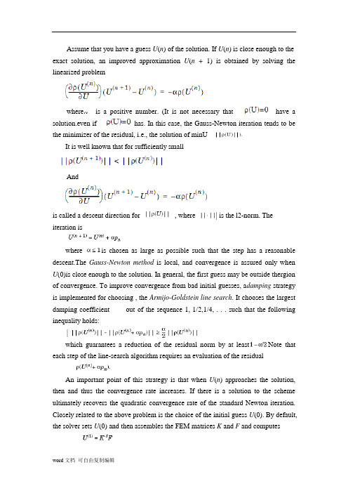
Assume that you have a guess U(n) of the solution. If U(n) is close enough to the exact solution, an improved approximation U(n + 1) is obtained by solving the linearized problemwhere have asolution.has. In this case, the Gauss-Newton iteration tends to be the minimizer of the residual, i.e., the solution of minUIt is well known that for sufficiently smallAndis called a descent direction for , where | is the l2-norm. The iteration iswhere is chosen as large as possible such that the step has a reasonable descent.The Gauss-Newton method is local, and convergence is assured only when U(0)is close enough to the solution. In general, the first guess may be outside thergion of convergence. To improve convergence from bad initial guesses, a damping strategy is implemented for choosing , the Armijo-Goldstein line search. It chooses the largestinequality holds:|which guarantees a reduction of the residual norm by at least Note that each step of the line-search algorithm requires an evaluation of the residualAn important point of this strategy is that when U(n) approaches the solution, then and thus the convergence rate increases. If there is a solution to the scheme ultimately recovers the quadratic convergence rate of the standard Newton iteration. Closely related to the above problem is the choice of the initial guess U(0). By default, the solver sets U(0) and then assembles the FEM matrices K and F and computesThe damped Gauss-Newton iteration is then started with U(1), which should be a better guess than U(0). If the boundary conditions do not depend on the solution u, then U(1) satisfies them even if U(0) does not. Furthermore, if the equation is linear, then U(1) is the exact FEM solution and the solver does not enter the Gauss-Newton loop.There are situations where U(0) = 0 makes no sense or convergence is impossible.In some situations you may already have a good approximation and the nonlinear solver can be started with it, avoiding the slow convergence regime.This idea is used in the adaptive mesh generator. It computes a solution on a mesh, evaluates the error, and may refine certain triangles. The interpolant of is a very good starting guess for the solution on the refined mesh.In general the exact Jacobianis not available. Approximation of Jn by finite differences in the following way is expensive but feasible. The ith column of Jn can be approximated bywhich implies the assembling of the FEM matrices for the triangles containing grid point i. A very simple approximation to Jn, which gives a fixed point iteration, is also possible as follows. Essentially, for a given U(n), compute the FEM matrices K and F and setNonlinear EquationsThis is equivalent to approximating the Jacobian with the stiffness matrix. Indeed, since putting Jn = K yields In many cases the convergence rate is slow, but the cost of each iteration is cheap.The nonlinear solver implemented in the PDE Toolbox also provides for a compromise between the two extremes. To compute the derivative of the mapping , proceed as follows. The a term has been omitted for clarity, but appears again in the final result below.The first integral term is nothing more than Ki,j.The second term is “lumped,” i.e., replaced by a diagonal matrix that contains the row j j = 1, the second term is approximated bywhich is the ith component of K(c')U, where K(c') is the stiffness matrixassociated with the coefficient rather than c. The same reasoning can beapplied to the derivative of the mapping . Finally note that thederivative of the mapping is exactlywhich is the mass matrix associated with the coefficient . Thus the Jacobian ofU) is approximated bywhere the differentiation is with respect to u. K and M designate stiffness and mass matrices and their indices designate the coefficients with respect to which they are assembled. At each Gauss-Newton iteration, the nonlinear solver assembles the matrices corresponding to the equationsand then produces the approximate Jacobian. The differentiations of the coefficients are done numerically.In the general setting of elliptic systems, the boundary conditions are appended to the stiffness matrix to form the full linear system: where the coefficients of and may depend on the solution . The “lumped”approach approximates the derivative mapping of the residual by The nonlinearities of the boundary conditions and the dependencies of the coefficients on the derivatives of are not properly linearized by this scheme. When such nonlinearities are strong, the scheme reduces to the fix-pointiter ation and may converge slowly or not at all. When the boundary condition sare linear, they do not affect the convergence properties of the iteration schemes. In the Neumann case they are invisible (H is an empty matrix) and in the Dirichlet case they merely state that the residual is zero on the corresponding boundary points.Adaptive Mesh RefinementThe toolbox has a function for global, uniform mesh refinement. It divides each triangle into four similar triangles by creating new corners at the midsides, adjusting for curved boundaries. You can assess the accuracy of the numerical solution by comparing results from a sequence of successively refined meshes.If the solution is smooth enough, more accurate results may be obtained by extra polation. The solutions of the toolbox equation often have geometric features like localized strong gradients. An example of engineering importance in elasticity is the stress concentration occurring at reentrant corners such as the MATLAB favorite, the L-shaped membrane. Then it is more economical to refine the mesh selectively, i.e., only where it is needed. When the selection is based ones timates of errors in the computed solutions, a posteriori estimates, we speak of adaptive mesh refinement. Seeadapt mesh for an example of the computational savings where global refinement needs more than 6000elements to compete with an adaptively refined mesh of 500 elements.The adaptive refinement generates a sequence of solutions on successively finer meshes, at each stage selecting and refining those elements that are judged to contribute most to the error. The process is terminated when the maximum number of elements is exceeded or when each triangle contributes less than a preset tolerance. You need to provide an initial mesh, and choose selection and termination criteria parameters. The initial mesh can be produced by the init mesh function. The three components of the algorithm are the error indicator function, which computes an estimate of the element error contribution, the mesh refiner, which selects and subdivides elements, and the termination criteria.The Error Indicator FunctionThe adaption is a feedback process. As such, it is easily applied to a lar gerrange of problems than those for which its design was tailored. You wantes timates, selection criteria, etc., to be optimal in the sense of giving the mostaccurate solution at fixed cost or lowest computational effort for a given accuracy. Such results have been proved only for model problems, butgenerally, the equid is tribution heuristic has been found near optimal. Element sizes should be chosen such that each element contributes the same to the error. The theory of adaptive schemes makes use of a priori bounds forsolutions in terms of the source function f. For none lli ptic problems such abound may not exist, while the refinement scheme is still well defined and has been found to work well.The error indicator function used in the toolbox is an element-wise estimate of the contribution, based on the work of C. Johnson et al. For Poisson'sequation –f -solution uh holds in the L2-normwhere h = h(x) is the local mesh size, andThe braced quantity is the jump in normal derivative of v hr is theEi, the set of all interior edges of thetrain gulation. This bound is turned into an element-wise error indicator function E(K) for element K by summing the contributions from its edges. The final form for the toolbox equation Becomeswhere n is the unit normal of edge and the braced term is the jump in flux across the element edge. The L2 norm is computed over the element K. This error indicator is computed by the pdejmps function.The Mesh RefinerThe PDE Toolbox is geared to elliptic problems. For reasons of accuracy and ill-conditioning, they require the elements not to deviate too much from beingequilateral. Thus, even at essentially one-dimensional solution features, such as boundary layers, the refinement technique must guarantee reasonably shaped triangles.When an element is refined, new nodes appear on its mid sides, and if the neighbor triangle is not refined in a similar way, it is said to have hanging nodes. The final triangulation must have no hanging nodes, and they are removed by splitting neighbor triangles. To avoid further deterioration oftriangle quality in successive generations, the “longest edge bisection” scheme Rosenberg-Stenger [8] is used, in which the longest side of a triangle is always split, whenever any of the sides have hanging nodes. This guarantees that no angle is ever smaller than half the smallest angle of the original triangulation. Two selection criteria can be used. One, pdead worst, refines all elements with value of the error indicator larger than half the worst of any element. The other, pdeadgsc, refines all elements with an indicator value exceeding a user-defined dimensionless tolerance. The comparison with the tolerance is properly scaled with respect to domain and solution size, etc.The Termination CriteriaFor smooth solutions, error equi distribution can be achieved by the pde adgsc selection if the maximum number of elements is large enough. The pdead worst adaption only terminates when the maximum number of elements has been exceeded. This mode is natural when the solution exhibits singularities. The error indicator of the elements next to the singularity may never vanish, regardless of element size.外文翻译假定估计值,如果是最接近的准确的求解,通过解决线性问题得到更精确的值当为正数时,( 有一个解,即使也有一个解都是不需要的。
数学专业外文翻译---幂级数的展开及其应用

数学专业外文翻译---幂级数的展开及其应用In the us n。
we XXX its convergence n。
a power series always converges to a n。
We can use simple power series。
as well as XXX quadrature methods。
to find this n。
However。
this n will address another issue: can an arbitrary n f(x) be expanded into a power series?XXX n will address this XXX power series can be seen as an n of reality。
so we can start to solve the problem of expanding a n f(x) into a power series by considering f(x) and polynomials。
To do this。
we will introduce the following formula without proof:Taylor'XXX that if a n f(x) has derivatives of order n+1 in a neighborhood of x=x0.then we can use the following XXX:f(x)=f(x0)+f'(x0)(x-x0)+f''(x0)(x-x0)^2+。
+f^(n)(x0)(x-x0)^n+r_n(x)Here。
r_n(x) represents the remainder term.XXX (x) is given by (x-x)n+1.This formula is of the (9-5-1) type for the Taylor series。
数学专业英语外文翻译

重庆理工大学数学专业英语学院学号姓名年月 2012年12月17日CONTROLLABILITY OF NEUTRAL FUNCTIONAL DIFFERENTIAL EQUATIONS WITH INFINITE DELA Y可控的无穷时滞中立型泛函微分方程In this article, we establish a result about controllability to the following class of partial neutral functional di fferential equations with infinite delay:0,),()(0≥⎪⎩⎪⎨⎧∈=++=∂∂t x xt t F t Cu ADxt Dxt t βφ (1)在这篇文章中,我们建立一个关于可控的结果偏中性与无限时滞泛函微分方程的下面的类: 0,),()(0≥⎪⎩⎪⎨⎧∈=++=∂∂t x xt t F t Cu ADxt Dxt tβφ (1) where the state variable (.)x takes values in a Banach space ).,(E and the control (.)u is given in[]0),,,0(2>T U T L ,the Banach space of admissible control functions with U a Banach space. C is abounded linear operator from U into E, A : D(A) ⊆ E → E is a linear operator on E, B is the phase space of functions mapping (−∞, 0] into E, which will be specified later, D is a bounded linear operator from B into E defined byB D D ∈-=ϕϕϕϕ,)0(0状态变量(.)x 在).,(E 空间值和控制用(.)u 受理控制范围[]0),,,0(2>T U T L 的Banach 空间,Banach 空间。
- 1、下载文档前请自行甄别文档内容的完整性,平台不提供额外的编辑、内容补充、找答案等附加服务。
- 2、"仅部分预览"的文档,不可在线预览部分如存在完整性等问题,可反馈申请退款(可完整预览的文档不适用该条件!)。
- 3、如文档侵犯您的权益,请联系客服反馈,我们会尽快为您处理(人工客服工作时间:9:00-18:30)。
第3章 最小均方算法3.1 引言最小均方(LMS ,least-mean-square)算法是一种搜索算法,它通过对目标函数进行适当的调整[1]—[2],简化了对梯度向量的计算。
由于其计算简单性,LMS 算法和其他与之相关的算法已经广泛应用于白适应滤波的各种应用中[3]-[7]。
为了确定保证稳定性的收敛因子范围,本章考察了LMS 算法的收敛特征。
研究表明,LMS 算法的收敛速度依赖于输入信号相关矩阵的特征值扩展[2]—[6]。
在本章中,讨论了LMS 算法的几个特性,包括在乎稳和非平稳环境下的失调[2]—[9]和跟踪性能[10]-[12]。
本章通过大量仿真举例对分析结果进行了证实。
在附录B 的B .1节中,通过对LMS 算法中的有限字长效应进行分析,对本章内容做了补充。
LMS 算法是自适应滤波理论中应用最广泛的算法,这有多方面的原因。
LMS 算法的主要特征包括低计算复杂度、在乎稳环境中的收敛性、其均值无俯地收敛到维纳解以及利用有限精度算法实现时的稳定特性等。
3.2 LMS 算法在第2章中,我们利用线性组合器实现自适应滤波器,并导出了其参数的最优解,这对应于多个输入信号的情形。
该解导致在估计参考信号以d()k 时的最小均方误差。
最优(维纳)解由下式给出:10w R p-= (3.1)其中,R=E[()x ()]Tx k k 且p=E[d()x()] k k ,假设d()k 和x()k 联合广义平稳过程。
如果可以得到矩阵R 和向量p 的较好估计,分别记为()R k ∧和()p k ∧,则可以利用如下最陡下降算法搜索式(3.1)的维纳解:w(+1)=w()-g ()w k k k μ∧w()(()()w())k p k R k k μ∧∧=-+2 (3.2) 其中,k =0,1,2,…,g ()w k ∧表示目标函数相对于滤波器系数的梯度向量估计值。
一种可能的解是通过利用R 和p 的瞬时估计值来估计梯度向量,即 ()x()x ()TR k k k ∧=()()x()p k d k k ∧= (3.3) 得到的梯度估计值为()2()x()2x()x ()()T w g k d k k k k w k ∧=-+2x()(()x ()())Tk d k k w k =-+ 2()x()e k k =- (3.4)注意,如果目标函数用瞬时平方误差2()e k 而不是MSE 代替,则上面的梯度估计值代表了真实梯度向量,因为2010()()()()2()2()2()()()()Te k e k e k e k e k e k e k w w k w k w k ⎡⎤∂∂∂∂=⎢⎥∂∂∂∂⎣⎦L2()x()e k k =-()w g k ∧= (3.5)由于得到的梯度算法使平方误差的均值最小化.因此它被称为LMS 算法,其更新方程为 (1)()2()x()w k w k e k k μ+=+ (3.6) 其中,收敛因子μ应该在一个范围内取值,以保证收敛性。
图3.1表示了对延迟线输入x()k 的LMS 算法实现。
典型情况是,LMS 算法的每次迭代需要N+2次乘法(用于滤波器系数的更新),而且还需要N+1次乘法(用于产生误差信号)。
LMS 算法的详细描述见算法3.1图3.1 LMS 自适应RH 滤波器算法3.1 LMS 算法Initializationx(0)(0)[000]T w ==LDo for 0k ≥()()x ()()Te k d k k w k =- (1)()2()x()w k w k e k k μ+=+需要指出的是,初始化并不一定要像在算法3.1小那样将白适应滤波器的系数被创始化为零:比如,如果知道最优系数的粗略值,则可以利用这些值构成w(0),这样可以减少到达0w 的邻域所需的迭代次数。
3.3 LMS 算法的一些特性在本节中,描述丁在平稳环境下与LMS 算法收敛特性相关的主要特性。
这里给出的信息对于理解收敛因子μ对LMS 算法的各个收敛方面的影响是很重要的。
3.3.1 梯度特性正如第2章中所指出的(见式(2.79)),在MSE 曲面上完成搜索最优系数向量解的理想梯度方向为()2{[x()x ()]()[()x()]}T w g k E k k w k E d k k =-2[()]Rw k p =- (3.7) 在LMS 算法中,利用R 和p 的瞬时估计值确定搜索方向,即()2[x()x ()()()x()]T w g k k k w k d k k ∧=- (3.8)正如所期望的,由式(3.8)所确定的方向与式(3.7)所确定的方向很不同。
因此,当通过利用LMS 算法计算更加有效的梯度方向时,收敛特性与最陡下降算法的收敛特性并不相同。
从平均的意义上讲,可以说LMS 梯度方向具有接近理想梯度方向的趋势,因为对于固定购系数向量w ,有[()]2{[x()x ()][()x()]}T w E g k E k k w E d k k ∧=-wg = (3.9)因此,向量g ()w k ∧可以解释为w g 的无偏瞬时估计值。
在具有遍历件的环境中,如果对于一个固定的w ,利用大量的输入和参考信号来计算向量g ()w k ∧,则平均方向趋近于w g ,即11lim ()MwwM i gk i g M∧→∞=+→∑ (3.10)3.3.2 系数向量的收敛特性假设一个系数向量为w 。
的未知FIR 滤波器,被一个具备相同阶数的白适应FIR 滤波器利用LMS 算法进行辨识。
在未知系统输出令附加了测量白噪声n(k),其均值为零,方差为2n σ。
在每一次迭代中,自适应滤波器系数相对于理想系数向量0w ,的误差由N+1维向量描述:0()()w k w k w ∆=- (3.11) 利用这种定义,LMS 算法也可以另外描述为 (1)()2()x()w k w k e k k μ∆+=∆+0()2x()[x ()x ()()]T Tw k k k w k w k μ=∆+-0()2x()[x ()()]Tw k k e k w k μ=∆+-∆0[2x()x ()]()2()x()TI k k w k e k k μμ=-∆+ (3.12)其中,0()e k 为最优输出误差.它由下式给出:00()()x()T e k d k w k =-00x()()x()T T w k n k w k =+-()n k = (3.13) 于是,系数向量中的期望误差为0[(1)]{[2x()x ()]()2[()x()]}T E w k E I k k w k E e k k μμ∆+=-∆+ (3.14)假设x()k 的元素与()w k ∆和0()e k 的元素统计独立,则式(314)可以简化为 [(1)]{2[x()x ()]}[()]TE w k I E k k E w k μ∆+=-∆(2)[()]I R E w k μ=-∆ (3.15) 如果我们假设参数的偏差只依赖于以前的输入信号向量,则第一个假设成立,而在第二个假设中,我们也考虑了最优解对应的误差信号与输入信号向量的元素正交。
由上述表达式可得1[(1)](2)[(0)]k E w k I R E w μ+∆+=-∆ (3.16)如果将式(3.15)左乘Q T(其中Q 为通过一个相似变换使R 对角化的酉矩阵),则可以得到 [(1)](2)[()]TTTE Q w k I Q RQ E Q w k μ∆+=-∆ '[(1)]E w k =∆+ '(2)[()]I E w k μ=-Λ∆1'1200012[()]0012N E w k μλμλμλ-⎡⎤⎢⎥-⎢⎥=∆⎢⎥⎢⎥-⎣⎦L M M M O M (3.17) 其中,'(1)(1)Tw k Q w k ∆+=∆+为旋转系数误差向量。
应用旋转可以得到一个产生对角矩阵的方程,从而更加易于分析方程的动态特性。
另外.上述关系可以表示为 '1'[(1)](2)[(0)]k E w k I E w μ+∆+=-Λ∆101'11(12)000(12)[(0)]00(12)k k k N E w μλμλμλ+++⎡⎤-⎢⎥-⎢⎥=∆⎢⎥⎢⎥-⎢⎥⎣⎦L M M M O M(3.18) 该方程说明.为了保证系数在平均意义上收敛,LMS 算法的收敛因子必须在如下范围内选取:max 10μλ<<(3.19)其中,max λ为R 的最大持征值。
在该范围内的μ值保证了当k →∞时,式(3.18)中对角矩阵的所有元素趋近于零.这是因为对于i =0,l ,…,N ,有1(12)1i μλ-<-<。
因此,对于较大的k 值,'[(1)]E w k ∆+趋近于零。
按照上述方法选取的μ值确保了系数向量的平均值接近于员优系数向量0w 比该指出的是,如果矩阵R 具有大的特征值扩展,则建议选择远小于上界μ值。
因此,系数的收敛速度将主要取决于最小特征值,它对应于式(3.18)中的最慢模式。
上述分析中的关键假设是所谓的独立件理论[4],它考虑了当i =0,1,…,k 时,所有向量()x i 均为统计独立的情况。
这个假设允许我们考虑在式(3.14)中()w k ∆独立于()x ()T x k k 。
尽管在x()k 由延迟线元素组成时,这个假设并不是非常有效,但是由它得到的理论结果与实验结果能够很好地吻合。
3.3.3 系数误差向量协方差矩阵在本节中,我们将推导得出自适应滤波器系数误差的二阶统计量表达式。
由于对于大的k 值,()w k ∆的平均值为零,因此系数误差向量的协方差的定义为00cov[()][()()]{[()][()]}T Tw k E w k w k E w k w w k w ∆=∆∆=-- (3.20)将式(3.12)代人式(3.20),可以得到cov[(1)]{[2x()x ()]()()[2x()x ()]T T T Tw k E I k k w k w k I k k μμ∆+=-∆∆-0[2x()x ()]()2()x ()T TI k k w k e k k μμ+-∆ 02()x ()()[2x()x ()]T T T Te k k w k I k k μμ+∆-2204()x()x ()}T e k k k μ+ (3.21)考虑到0()e k 独立于()w k ∆且正交于()x k ,因此上式中右边第二项和第三项可以消除。
可以通过描述被消除的矩阵的每一个元素来说明这种简化的详细过程。
在这种情况下, cov[(1)]cov[()][2x()x ()()()TTw k w k E k k w k w k μ∆+=∆+-∆∆ 2()()x()x ()TTw k w k k k μ-∆∆ 24x()x ()()()TTk k w k w k μ+∆∆2204()x()x ()]T e k k k μ+ (3.22)另外,假设()w k ∆独立于x()k ,则式(3.22)可以重新写为cov[(1)]cov[()]2[x()x ()][()()]TTw k w k E k k E w k w k μ∆+=∆-∆∆ 2[()()][x()x ()]TT E w k w k E k k μ-∆∆ 24E{x()x ()()()}TTk k w k w k μ+∆∆2204[()x()x ()]T E e k k k μ+cov[()]2cov[()]w k R w k μ=∆-∆2222cov[()]44n w k R A R μμμσ-∆++ (3.23)计算式E{x()x ()[()()]x()x ()}T T TA k k E w k w k k k =∆∆包括了四阶矩,对于联合高斯输人信号样值,可以采用文献[4],[13]中描述的方法。