General Terms Algorithms.
Gravitation-Based Model for Information Retrieval

ABSTRACT
This paper proposes GBM (gravitation-based model), a physical model for information retrieval inspired by Newton’s theory of gravitation. A mapping is built in this model from concepts of information retrieval (documents, queries, relevance, etc) to those of physics (mass, distance, radius, attractive force, etc). This model actually provides a new perspective on IR problems. A family of effective term weighting functions can be derived from it, including the well-known BM25 formula. This model has some advantages over most existing ones: First, because it is directly based on basic physical laws, the derived formulas and algorithms can have their explicit physical interpretation. Second, the ranking formulas derived from this model satisfy more intuitive heuristics than most of existing ones, thus have the potential to behave empirically better and to be used safely on various settings. Finally, a new approach for structured document retrieval derived from this model is more reasonable and behaves better than existing ones.
stoerwagner-mincut.[Stoer-Wagner,Prim,连通性,无向图,最小边割集]
![stoerwagner-mincut.[Stoer-Wagner,Prim,连通性,无向图,最小边割集]](https://img.taocdn.com/s3/m/072209d5360cba1aa811da51.png)
A Simple Min-Cut AlgorithmMECHTHILD STOERTeleverkets Forskningsinstitutt,Kjeller,NorwayANDFRANK WAGNERFreie Universita¨t Berlin,Berlin-Dahlem,GermanyAbstract.We present an algorithm for finding the minimum cut of an undirected edge-weighted graph.It is simple in every respect.It has a short and compact description,is easy to implement,and has a surprisingly simple proof of correctness.Its runtime matches that of the fastest algorithm known.The runtime analysis is straightforward.In contrast to nearly all approaches so far,the algorithm uses no flow techniques.Roughly speaking,the algorithm consists of about͉V͉nearly identical phases each of which is a maximum adjacency search.Categories and Subject Descriptors:G.L.2[Discrete Mathematics]:Graph Theory—graph algorithms General Terms:AlgorithmsAdditional Key Words and Phrases:Min-Cut1.IntroductionGraph connectivity is one of the classical subjects in graph theory,and has many practical applications,for example,in chip and circuit design,reliability of communication networks,transportation planning,and cluster analysis.Finding the minimum cut of an undirected edge-weighted graph is a fundamental algorithmical problem.Precisely,it consists in finding a nontrivial partition of the graphs vertex set V into two parts such that the cut weight,the sum of the weights of the edges connecting the two parts,is minimum.A preliminary version of this paper appeared in Proceedings of the2nd Annual European Symposium on Algorithms.Lecture Notes in Computer Science,vol.855,1994,pp.141–147.This work was supported by the ESPRIT BRA Project ALCOM II.Authors’addresses:M.Stoer,Televerkets Forskningsinstitutt,Postboks83,2007Kjeller,Norway; e-mail:mechthild.stoer@nta.no.;F.Wagner,Institut fu¨r Informatik,Fachbereich Mathematik und Informatik,Freie Universita¨t Berlin,Takustraße9,Berlin-Dahlem,Germany;e-mail:wagner@inf.fu-berlin.de.Permission to make digital/hard copy of part or all of this work for personal or classroom use is granted without fee provided that the copies are not made or distributed for profit or commercial advantage,the copyright notice,the title of the publication,and its date appear,and notice is given that copying is by permission of the Association for Computing Machinery(ACM),Inc.To copy otherwise,to republish,to post on servers,or to redistribute to lists,requires prior specific permission and/or a fee.᭧1997ACM0004-5411/97/0700-0585$03.50Journal of the ACM,Vol.44,No.4,July1997,pp.585–591.586M.STOER AND F.WAGNER The usual approach to solve this problem is to use its close relationship to the maximum flow problem.The famous Max-Flow-Min-Cut-Theorem by Ford and Fulkerson[1956]showed the duality of the maximum flow and the so-called minimum s-t-cut.There,s and t are two vertices that are the source and the sink in the flow problem and have to be separated by the cut,that is,they have to lie in different parts of the partition.Until recently all cut algorithms were essentially flow algorithms using this duality.Finding a minimum cut without specified vertices to be separated can be done by finding minimum s-t-cuts for a fixed vertex s and all͉V͉Ϫ1possible choices of tʦVگ{s}and then selecting the lightest one.Recently Hao and Orlin[1992]showed how to use the maximum flow algorithm by Goldberg and Tarjan[1988]in order to solve the minimum cut problem in timeᏻ(͉VʈE͉log(͉V͉2/͉E͉),which is nearly as fast as the fastest maximum flow algorithms so far[Alon1990;Ahuja et al.1989;Cheriyan et al. 1990].Nagamochi and Ibaraki[1992a]published the first deterministic minimum cut algorithm that is not based on a flow algorithm,has the slightly better running time ofᏻ(͉VʈE͉ϩ͉V͉2log͉V͉),but is still rather complicated.In the unweighted case,they use a fast-search technique to decompose a graph’s edge set E into subsets E1,...,Esuch that the union of the first k E i’s is a k-edge-connected spanning subgraph of the given graph and has at most k͉V͉edges.They simulate this approach in the weighted case.Their work is one of a small number of papers treating questions of graph connectivity by non-flow-based methods [Nishizeki and Poljak1989;Nagamochi and Ibaraki1992a;Matula1992].Karger and Stein[1993]suggest a randomized algorithm that with high probability finds a minimum cut in timeᏻ(͉V͉2log͉V͉).In this context,we present in this paper a remarkably simple deterministic minimum cut algorithm with the fastest running time so far,established in Nagamochi and Ibaraki[1992b].We reduce the complexity of the algorithm of Nagamochi and Ibaraki by avoiding the unnecessary simulated decomposition of the edge set.This enables us to give a comparably straightforward proof of correctness avoiding,for example,the distinction between the unweighted, integer-,rational-,and real-weighted case.This algorithm was found independently by Frank[1994].Queyranne[1995]generalizes our simple approach to the minimization of submodular functions.The algorithm described in this paper was implemented by Kurt Mehlhorn from the Max-Planck-Institut,Saarbru¨cken and is part of the algorithms library LEDA[Mehlhorn and Na¨her1995].2.The AlgorithmThroughout the paper,we deal with an ordinary undirected graph G with vertex set V and edge set E.Every edge e has nonnegative real weight w(e).The simple key observation is that,if we know how to find two vertices s and t, and the weight of a minimum s-t-cut,we are nearly done:T HEOREM2.1.Let s and t be two vertices of a graph G.Let G/{s,t}be the graph obtained by merging s and t.Then a minimum cut of G can be obtained by taking the smaller of a minimum s-t-cut of G and a minimum cut of G/{s,t}.The theorem holds since either there is a minimum cut of G that separates s and t ,then a minimum s -t -cut of G is a minimum cut of G ;or there is none,then a minimum cut of G /{s ,t }does the job.So a procedure finding an arbitrary minimum s -t -cut can be used to construct a recursive algorithm to find a minimum cut of a graph.The following algorithm,known in the literature as maximum adjacency search or maximum cardinality search ,yields the desired s -t -cut.M INIMUM C UT P HASE (G ,w ,a )A 4{a }while A Vadd to A the most tightly connected vertexstore the cut-of-the-phase and shrink G by merging the two vertices added lastA subset A of the graphs vertices grows starting with an arbitrary single vertex until A is equal to V .In each step,the vertex outside of A most tightly connected with A is added.Formally,we add a vertexz ʦ͞A such that w ͑A ,z ͒ϭmax ͕w ͑A ,y ͉͒y ʦ͞A ͖,where w (A ,y )is the sum of the weights of all the edges between A and y .At the end of each such phase,the two vertices added last are merged ,that is,the two vertices are replaced by a new vertex,and any edges from the two vertices to a remaining vertex are replaced by an edge weighted by the sum of the weights of the previous two edges.Edges joining the merged nodes are removed.The cut of V that separates the vertex added last from the rest of the graph is called the cut-of-the-phase .The lightest of these cuts-of-the-phase is the result of the algorithm,the desired minimum cut:M INIMUM C UT (G ,w ,a )while ͉V ͉Ͼ1M INIMUM C UT P HASE (G ,w ,a )if the cut-of-the-phase is lighter than the current minimum cutthen store the cut-of-the-phase as the current minimum cutNotice that the starting vertex a stays the same throughout the whole algorithm.It can be selected arbitrarily in each phase instead.3.CorrectnessIn order to proof the correctness of our algorithms,we need to show the following somewhat surprising lemma.L EMMA 3.1.Each cut -of -the -phase is a minimum s -t -cut in the current graph ,where s and t are the two vertices added last in the phase .P ROOF .The run of a M INIMUM C UT P HASE orders the vertices of the current graph linearly,starting with a and ending with s and t ,according to their order of addition to A .Now we look at an arbitrary s -t -cut C of the current graph and show,that it is at least as heavy as the cut-of-the-phase.587A Simple Min-Cut Algorithm588M.STOER AND F.WAGNER We call a vertex v a active(with respect to C)when v and the vertex added just before v are in the two different parts of C.Let w(C)be the weight of C,A v the set of all vertices added before v(excluding v),C v the cut of A vഫ{v} induced by C,and w(C v)the weight of the induced cut.We show that for every active vertex vw͑A v,v͒Յw͑C v͒by induction on the set of active vertices:For the first active vertex,the inequality is satisfied with equality.Let the inequality be true for all active vertices added up to the active vertex v,and let u be the next active vertex that is added.Then we havew͑A u,u͒ϭw͑A v,u͒ϩw͑A uگA v,u͒ϭ:␣Now,w(A v,u)Յw(A v,v)as v was chosen as the vertex most tightly connected with A v.By induction w(A v,v)Յw(C v).All edges between A uگA v and u connect the different parts of C.Thus they contribute to w(C u)but not to w(C v).So␣Յw͑C v͒ϩw͑A uگA v,u͒Յw͑C u͒As t is always an active vertex with respect to C we can conclude that w(A t,t)Յw(C t)which says exactly that the cut-of-the-phase is at most as heavy as C.4.Running TimeAs the running time of the algorithm M INIMUM C UT is essentially equal to the added running time of the͉V͉Ϫ1runs of M INIMUM C UT P HASE,which is called on graphs with decreasing number of vertices and edges,it suffices to show that a single M INIMUM C UT P HASE needs at mostᏻ(͉E͉ϩ͉V͉log͉V͉)time yielding an overall running time ofᏻ(͉VʈE͉ϩ͉V͉2log͉V͉).The key to implementing a phase efficiently is to make it easy to select the next vertex to be added to the set A,the most tightly connected vertex.During execution of a phase,all vertices that are not in A reside in a priority queue based on a key field.The key of a vertex v is the sum of the weights of the edges connecting it to the current A,that is,w(A,v).Whenever a vertex v is added to A we have to perform an update of the queue.v has to be deleted from the queue,and the key of every vertex w not in A,connected to v has to be increased by the weight of the edge v w,if it exists.As this is done exactly once for every edge,overall we have to perform͉V͉E XTRACT M AX and͉E͉I NCREASE K EY ing Fibonacci heaps[Fredman and Tarjun1987],we can perform an E XTRACT M AX operation inᏻ(log͉V͉)amortized time and an I NCREASE K EY operation inᏻ(1)amortized time.Thus,the time we need for this key step that dominates the rest of the phase, isᏻ(͉E͉ϩ͉V͉log͉V͉).5.AnExample F IG .1.A graph G ϭ(V ,E )withedge-weights.F IG .2.The graph after the first M INIMUM C UT P HASE (G ,w ,a ),a ϭ2,and the induced ordering a ,b ,c ,d ,e ,f ,s ,t of the vertices.The first cut-of-the-phase corresponds to the partition {1},{2,3,4,5,6,7,8}of V with weight w ϭ5.F IG .3.The graph after the second M INIMUM C UT P HASE (G ,w ,a ),and the induced ordering a ,b ,c ,d ,e ,s ,t of the vertices.The second cut-of-the-phase corresponds to the partition {8},{1,2,3,4,5,6,7}of V with weight w ϭ5.F IG .4.After the third M INIMUM C UT P HASE (G ,w ,a ).The third cut-of-the-phase corresponds to the partition {7,8},{1,2,3,4,5,6}of V with weight w ϭ7.589A Simple Min-Cut AlgorithmACKNOWLEDGMENT .The authors thank Dorothea Wagner for her helpful re-marks.REFERENCESA HUJA ,R.K.,O RLIN ,J.B.,AND T ARJAN ,R.E.1989.Improved time bounds for the maximum flow problem.SIAM put.18,939–954.A LON ,N.1990.Generating pseudo-random permutations and maximum flow algorithms.Inf.Proc.Lett.35,201–204.C HERIYAN ,J.,H AGERUP ,T.,AND M EHLHORN ,K.1990.Can a maximum flow be computed in o (nm )time?In Proceedings of the 17th International Colloquium on Automata,Languages and Programming .pp.235–248.F ORD ,L.R.,AND F ULKERSON ,D.R.1956.Maximal flow through a network.Can.J.Math.8,399–404.F RANK , A.1994.On the Edge-Connectivity Algorithm of Nagamochi and Ibaraki .Laboratoire Artemis,IMAG,Universite ´J.Fourier,Grenoble,Switzerland.F REDMAN ,M.L.,AND T ARJAN ,R.E.1987.Fibonacci heaps and their uses in improved network optimization algorithms.J.ACM 34,3(July),596–615.G OLDBERG ,A.V.,AND T ARJAN ,R.E.1988.A new approach to the maximum-flow problem.J.ACM 35,4(Oct.),921–940.H AO ,J.,AND O RLIN ,J.B.1992.A faster algorithm for finding the minimum cut in a graph.In Proceedings of the 3rd ACM-SIAM Symposium on Discrete Algorithms (Orlando,Fla.,Jan.27–29).ACM,New York,pp.165–174.K ARGER ,D.,AND S TEIN ,C.1993.An O˜(n 2)algorithm for minimum cuts.In Proceedings of the 25th ACM Symposium on the Theory of Computing (San Diego,Calif.,May 16–18).ACM,New York,pp.757–765.F IG .5.After the fourth and fifth M INIMUM C UT P HASE (G ,w ,a ),respectively.The fourth cut-of-the-phase corresponds to the partition {4,7,8},{1,2,3,5,6}.The fifth cut-of-the-phase corresponds to the partition {3,4,7,8},{1,2,5,6}with weight w ϭ4.F IG .6.After the sixth and seventh M INIMUM C UT P HASE (G ,w ,a ),respectively.The sixth cut-of-the-phase corresponds to the partition {1,5},{2,3,4,6,7,8}with weight w ϭ7.The last cut-of-the-phase corresponds to the partition {2},V گ{2};its weight is w ϭ9.The minimum cut of the graph G is the fifth cut-of-the-phase and the weight is w ϭ4.590M.STOER AND F.WAGNERM ATULA ,D.W.1993.A linear time 2ϩ⑀approximation algorithm for edge connectivity.In Proceedings of the 4th ACM–SIAM Symposium on Discrete Mathematics ACM,New York,pp.500–504.M EHLHORN ,K.,AND N ¨AHER ,S.1995.LEDA:a platform for combinatorial and geometric mun.ACM 38,96–102.N AGAMOCHI ,H.,AND I BARAKI ,T.1992a.Linear time algorithms for finding a sparse k -connected spanning subgraph of a k -connected graph.Algorithmica 7,583–596.N AGAMOCHI ,H.,AND I BARAKI ,puting edge-connectivity in multigraphs and capaci-tated graphs.SIAM J.Disc.Math.5,54–66.N ISHIZEKI ,T.,AND P OLJAK ,S.1989.Highly connected factors with a small number of edges.Preprint.Q UEYRANNE ,M.1995.A combinatorial algorithm for minimizing symmetric submodular functions.In Proceedings of the 6th ACM–SIAM Symposium on Discrete Mathematics ACM,New York,pp.98–101.RECEIVED APRIL 1995;REVISED FEBRUARY 1997;ACCEPTED JUNE 1997Journal of the ACM,Vol.44,No.4,July 1997.591A Simple Min-Cut Algorithm。
General Terms
The University of Amsterdam at WebCLEF2006Krisztian Balog Maarten de RijkeISLA,University of Amsterdamkbalog,mdr@science.uva.nlAbstractOur aim for our participation in WebCLEF2006was to investigate the robustness ofinformation retrieval techniques to crosslingual retrieval,such as compact documentrepresentations,and query reformulation techniques.Our focus was on the mixedmonolingual task.Apart from the proper preprocessing and transformation of variousencodings,we did not apply any language-specific techniques.Instead,the targetdomain metafield was used in some of our runs.A standard combSUM combinationusing Min-Max normalization was used to combine runs,based on a separate contentand title indexes of documents.We found that the combination is effective only forthe human generated topics.Query reformulation techniques can be used to improveretrieval performance,as witnessed by our best scoring configuration,however thesetechniques are not yet beneficial to all different kinds of topics.Categories and Subject DescriptorsH.3[Information Storage and Retrieval]:H.3.1Content Analysis and Indexing;H.3.3Infor-mation Search and Retrieval;H.3.4Systems and Software;H.3.7Digital Libraries;H.2.3[Database Managment]:Languages—Query LanguagesGeneral TermsMeasurement,Performance,ExperimentationKeywordsWeb retrieval,Multilingual retrieval1IntroductionThe world wide web is a natural setting for cross-lingual information retrieval,since the web content is essentially multilingual.On the other hand,web data is much noisier than traditional collections, eg.newswire or newspaper data,which originated from a single source.Also,the linguistic variety in the collection makes it harder to apply language-dependent processing methods,eg.stemming algorithms.Moreover,the size of the web only allows for methods that scale well.We investigate a range of approaches to crosslingual web retrieval using the test suite of the CLEF2006WebCLEF track,featuring a stream of known-item topics in various languages.The topics are a mixture of human generated(manually)and automatically generated topics.Our focus is on the mixed monolingual task.Our aim for our participation in WebCLEF2006was to investigate the robustness of information retrieval techniques,such as compact document repre-sentations(titles or incoming anchor-texts),and query reformulation techniques.The remainder of the paper is organized as follows.In Section2we describe our retrieval system as well as the specific approaches we applied.In Section3we describe the runs that we submitted,while the results of those runs are detailed in Section4.We conclude in Section5.2System DescriptionOur retrieval system is based on the Lucene engine[4].For our ranking,we used the default similarity measure of Lucene,i.e.,for a collection D, document d and query q containing terms t i:sim(q,d)=t∈q tf t,q·idf tnorm q·tf t,d·idf tnorm d·coord q,d·weight t,wheretf t,X=freq(t,X),idf t=1+log|D| freq(t,D),norm d= |d|,coord q,d=|q∩d||q|,andnorm q=t∈qtf t,q·idf t2.We did not apply any stemming nor did we use a stopword list.We applied case-folding and normalized marked characters to their unmarked counterparts,i.e.,mapping´a to a,¨o to o,æto ae,ˆıto i,etc.The only language specific processing we did was a transformation of the multiple Russian and Greek encodings into an ASCII transliteration.We extracted the full text from the documents,together with the title and anchorfields,and created three separate indexes:•Content:Index of the full document text.•Title:Index of all<title>fields.•Anchors:Index of all incoming anchor-texts.We performed three base runs using the separate indexes.We evaluated the base runs using the WebCLEF2005topics,and decided to use only the content and title indexes.2.1Run combinationsWe experimented with the combination of content and title runs,using standard combination methods as introduced by Fox and Shaw[1]:combMAX(take the maximal similarity score of the individual runs);combMIN(take the minimal similarity score of the individual runs);combSUM(take the sum of the similarity scores of the individual runs);combANZ(take the sum of the similarity scores of the individual runs,and divide by the number of non-zero entries);combMNZ(take the sum of the similarity scores of the individual runs,and multiply by the number of non-zero entries); and combMED(take the median similarity score of the individual runs).Fox and Shaw[1]found combSUM to be the best performing combination method.Kamps and de Rijke[2]conducted extensive experiments with the Fox and Shaw combination rules for nine european languages,and demonstrated that combination can lead into significant improvements.Moreover,they proved that the effectiveness of combining retrieval strategies differs between En-glish and other European languages.In Kamps and de Rijke[2],combSUM emerges as the best combination rule,confirming Fox and Shaw’sfindings.Similarity score distributions may differ radically across runs.We apply the combination methods to normalized similarity scores.That is,we follow Lee[3]and normalize retrieval scores into a[0,1]range,using the minimal and maximal similarity scores(min-max normalization):s =s−minmax−min,(1)where s denotes the original retrieval score,and min(max)is the minimal(maximal)score over all topics in the run.For the WebCLEF2005topics the best performance was achieved using the combSUM combi-nation rule,which is in conjunction with thefindings in[1,2],therefore we used that method for our WebCLEF2006submissions.2.2Query reformulationIn addition to our run combination experiments,we conducted experiments to measure the effect of phrase and query operations.We tested query-rewrite heuristics using phrases and word n-grams.Phrases In this straightforward mechanism we simply add the topic terms as a phrase to the topic.For example,for the topic WC0601907,with title“diana memorial fountain”,the query becomes:diana memorial fountain“diana memorial fountain”.Our intuition is that rewarding documents that contain the whole topic as a phrase,not only the individual terms,would be beneficial to retrieval performance.N-grams In our approach every word n-gram from the query is added to the query as a phrase with weight n.This means that longer phrases get bigger ing the previous topic as an example,the query becomes:diana memorial fountain“diana memorial”2“memorial fountain”2“diana memorial fountain”3,where the number in the upper index denotes the weight attached to the phrase(the weight of the individual terms is1).3RunsWe submittedfive runs to the mixed monolingual task:Baseline Base run using the content only index.Comb Combination of the content and title runs,using the CombSUM method.CombMeta The Comb run,using the target domain metafield.We restrict our search to the corresponding domain.CombPhrase The CombMeta run,using the Phrase query reformulation technique. CombNboost The CombMeta run,using the N-grams query reformulation technique.4ResultsTable1lists our results in terms of mean reciprocal rank.Runs are listed along the left-hand side,while the labels indicate either all topics(all)or various subsets:automatically generated (auto)—further subdivided into automatically generated using the unigram generator(auto-u) and automatically generated using the bigram generator(auto-b)—and manual(manual),which is further subdivided into new manual topics and old manual topics.Significance testing was done using the two-tailed Wilcoxon Matched-pair Signed-Ranks Test, where we look for improvements at a significance level of0.05(1),0.001(2),and0.0001(3). Signficant differences noted in Table1are with respect to the Baseline run.Table1:Submission results(Mean Reciprocal Rank)runID all auto auto-u auto-b manual man-n man-oBaseline0.16940.12530.13970.11100.39340.47870.3391Comb0.168510.120830.139430.10210.41120.49520.3578CombMeta0.194730.150530.167030.134130.418830.510810.36031 CombPhrase0.200130.157030.163930.150030.41900.51380.3587CombNboost0.195430.158630.159530.157630.38260.48910.3148Combination of the content and title runs(Comb)increased performance only for the manual topics.The use of the title tag does not help when the topics are automatically generated. Instead of employing a language detection method,we simply used the target domain metafield. The CombMeta run improved the retrieval performance significantly for all subsets of topics.Our query reformulation techniques show mixed,but promising results.The best overall score was achieved when the topic,as a phrase,was added to the query(CombPhrase).The comparison of CombPhrase vs CombMeta reveals that they achieved similar scores for all subsets of topics,except for the automatic topics using the bigram generator,where the query reformulation technique was clearly beneficial.The n-gram query reformulation technique(CombNboost)further improved the results of the auto-b topics,but hurt accuracy on all other subsets,especially on the manual topics. The CombPhrase run demonstrates that even a very simple query reformulation technique can be used to improve retrieval scores.However,we need to further investigate how to automatically detect whether it is beneficial to use such techniques(and if yes,which technique to apply)for a given a topic.Comparing the various subsets of topics,we see that the automatic topics have proven to be more difficult than the manual ones.Also,the new manual topics seem to be more appropriate for known-item search than the old manual topics.There is a clear ranking among the various subsets of topics,and this ranking is independent from the applied methods:man−n man−o auto−u auto−b.5ConclusionsOur aim for our participation in WebCLEF2006was to investigate the robustness of information retrieval techniques to crosslingual web retrieval.The only language-specific processing we applied was the transformation of various encodings into an ASCII transliteration.We did not apply any stemming nor did we use a stopword list.We indexed the collection by extracting the full text and the titlefields from the documents.A standard combSUM combination using Min-Max normalization was used to combine the runs based on the content and title indexes.We found that the combination is effective only for the human generated topics,using the titlefield did not improve performance when the topics are automatically generated.Significant improvements (+15%MRR)were achieved by using the target domain metafield.We also investigated the effect of query reformulation techniques.We found,that even very simple methods can improve retrieval performance,however these techniques are not yet beneficial to retrieval for all subsets of topics.Although it may be too early to talk about a solved problem,effective and robust web retrieval techniques seem to carry over to the mixed monolingual setting.6AcknowledgmentsKrisztian Balog was supported by the Netherlands Organisation for Scientific Research(NWO)un-der project numbers220-80-001,600.-065.-120and612.000.106.Maarten de Rijke was supported by NWO under project numbers017.001.190,220-80-001,264-70-050,354-20-005,600.-065.-120, 612-13-001,612.000.106,612.066.302,612.069.006,640.001.501,and640.002.501. References[1]E.Fox and bination of multiple searches.In The Second Text REtrieval Con-ference(TREC-2),pages243–252.National Institute for Standards and Technology.NIST Special Publication500-215,1994.[2]J.Kamps and M.de Rijke.The effectiveness of combining information retrieval strategiesfor European languages.In Proceedings of the2004ACM Symposium on Applied Computing, pages1073–1077,2004.[3]bining multiple evidence from different properties of weighting schemes.InSIGIR’95:Proceedings of the18th annual international ACM SIGIR conference on Research and development in information retrieval,pages180–188,New York,NY,USA,1995.ACM Press.ISBN0-89791-714-6.doi:/10.1145/215206.215358.[4]Lucene.The Lucene search engine,2005./.。
Boid规则
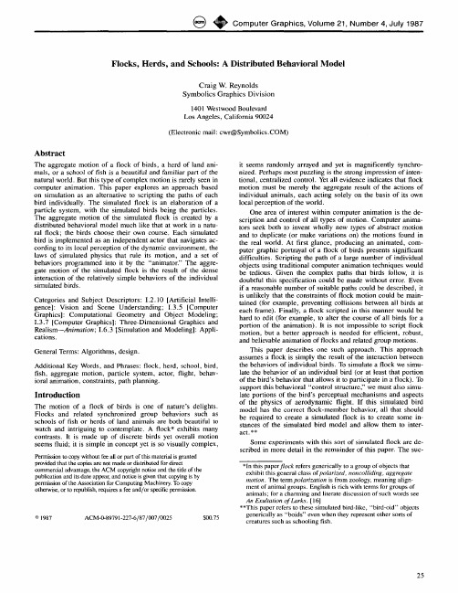
Abstract
The aggregate motion of a flock of birds, a herd of land animals, or a school of fish is a beautiful and familiar part of the n a t u r a l world. But this type of complex motion is rarely seen in computer animation. This paper explores an approach based on simulation as an alternative to scripting the paths of each bird individually. The simulated flock is an elaboration of a particle system, with the simulated birds being the particles. The aggregate motion of the simulated flock is created by a distributed behavioral model much like that at work in a natural flock; the birds choose their own course. Each simulated bird is implemented as an independent actor that navigates according to its local perception of the dynamic environment, the laws of simulated physics that rule its motion, and a set of behaviors programmed into it by the "animator." The aggregate motion of the simulated flock is the result of the dense interaction of the relatively simple behaviors of the individual simulated birds. Categories and Subject Descriptors: 1.2.10 [Artificial Intelligence]: Vision and Scene Understanding; 1.3.5 [Computer Graphics]: Computational Geometry and Object Modeling; 1.3.7 [Computer Graphics]: Three-Dimensional Graphics and Realism--Animation; 1.6.3 [Simulation and Modeling[: Applications. General Terms: Algorithms, design. Additional Key Words, and Phrases: flock, herd, school, bird, fish, aggregate motion, particle system, actor, flight, behavioral animation, constraints, path planning. it seems randomly arrayed and yet is magnificently synchronized. Perhaps most puzzling is the strong impression of intentional, centralized control. Yet all evidence indicates that flock motion must be merely the aggregate result of the actions of individual animals, each acting solely on the basis of its own local perception of the world. One area of interest within computer animation is the description and control of all types of motion. Computer animators seek both to invent wholly new types of abstract motion and to duplicate (or make variations on) the motions found in the real world. At first glance, producing an animated, computer graphic portrayal of a flock of birds presents significant difficulties. Scripting the path of a large number of individual objects using traditional computer animation techniques would be tedious. Given the complex paths that birds follow, it is doubtful this specification could be made without error. Even if a reasonable number of suitable paths could be described, it is unlikely that the constraints of flock motion could be maintained (for example, preventing collisions between all birds at each frame). Finally, a flock scripted in this manner would be hard to edit (for example, to alter the course of all birds for a portion of the animation). It is not impossible to script flock motion, but a better approach is needed for efficient, robust, and believable animation of flocks and related group motions. This paper describes one such approach. This approach assumes a flock is simply the result of the interaction between the behaviors of individual birds. To simulate a flock we simulate the behavior of an individual bird (or at least that portion of the bird's behavior that allows it to participate in a flock). To support this behavioral "control structure" we must also simulate portions of the bird's perceptual mechanisms and aspects of the physics of aerodynamic flight. If this simulated bird model has the correct flock-member behavior, all that should be required to create a simulated flock is to create some instances of the simulated bird model and allow them to interact. ** Some experiments with this sort of simulated flock are described in more detail in the remainder of this paper. The suc*In this paperflock refers generically to a group of objects that exhibit this general class of polarized, noncolliding, aggregate motion. The term polarization is from zoology, meaning alignment of animal groups. English is rich with terms for groups of animals; for a charming and literate discussion of such words see An Exultation of Larks. [16] **This paper refers to these simulated bird-like, "bird-old" objects generically as "boids" even when they represent other sorts of creatures such as schooling fish.
cuda bfs

Accelerating CUDA Graph Algorithms at Maximum WarpSungpack Hong Sang Kyun Kim Tayo Oguntebi Kunle OlukotunComputer Systems LaboratoryStanford University{hongsup,skkim38,tayo,kunle}@AbstractGraphs are powerful data representations favored in many compu-tational domains.Modern GPUs have recently shown promising re-sults in accelerating computationally challenging graph problems but their performance suffers heavily when the graph structure is highly irregular,as most real-world graphs tend to be.In this study, wefirst observe that the poor performance is caused by work imbal-ance and is an artifact of a discrepancy between the GPU program-ming model and the underlying GPU architecture.We then propose a novel virtual warp-centric programming method that exposes the traits of underlying GPU architectures to users.Our method signif-icantly improves the performance of applications with heavily im-balanced workloads,and enables trade-offs between workload im-balance and ALU underutilization forfine-tuning the performance.Our evaluation reveals that our method exhibits up to9x speedup over previous GPU algorithms and12x over single thread CPU execution on irregular graphs.When properly configured,it also yields up to30%improvement over previous GPU algorithms on regular graphs.In addition to performance gains on graph algo-rithms,our programming method achieves1.3x to15.1x speedup on a set of GPU benchmark applications.Our study also confirms that the performance gap between GPUs and other multi-threaded CPU graph implementations is primarily due to the large difference in memory bandwidth.Categories and Subject Descriptors D.1.3[Programming Tech-niques]:Concurrent Programming–Parallel programming; D.3.3 [Programming Languages]:Language Constructs and Features–PatternsGeneral Terms Algorithms,PerformanceKeywords Parallel graph algorithms,CUDA,GPGPU1.IntroductionGraphs are widely-used data structures that describe a set of ob-jects,referred to as nodes,and the connections between them, called edges.Certain graph algorithms,such as breadth-first search, minimum spanning tree,and shortest paths,serve as key compo-nents to a large number of applications[4,5,15–17,22,25]and have thus been heavily explored for potential improvement.Despite the considerable research conducted on making these algorithms Permission to make digital or hard copies of all or part of this work for personal or classroom use is granted without fee provided that copies are not made or distributed for profit or commercial advantage and that copies bear this notice and the full citation on thefirst page.To copy otherwise,to republish,to post on servers or to redistribute to lists,requires prior specific permission and/or a fee.PPoPP’11,Feb12–16,2011,San Antonio,Texas,USA.Copyright©2011ACM978-1-4503-01190-0/11/02...$10.00efficient,and the significant performance benefits they have reaped due to ever-increasing computational power,processing large irreg-ular graphs quickly and effectively remains an immense challenge today.Unfortunately,many real-world applications involve large irregular graphs.It is therefore important to fully exploit thefine-grain parallelism in these algorithms,especially as parallel compu-tation resources are abundant in modern CPUs and GPUs.The Parallel Random Access Machine(PRAM)abstraction has often been used to investigate theoretical parallel performance of graph algorithms[18].The PRAM abstraction assumes an infinite number of processors and unit latency to shared memory from any of the processors.Actual hardware approximations of PRAM,how-ever,have been rare.Conventional CPUs lack in number of pro-cessors,and clusters of commodity general-purpose processors are poorly-suited as PRAM approximations due to their large inter-node communication latencies.In addition,clusters which span multiple address spaces impose the added difficulty of partitioning the graphs.In the supercomputer domain,several accurate approx-imations of the PRAM,such as the Cray XMT[13],have demon-strated impressive performance executing sophisticated graph al-gorithms[5,17].Unfortunately,such machines are prohibitively costly for many organizations.GPUs have recently become popular as general computing de-vices due to their relatively low costs,massively parallel architec-tures,and improving accessibility provided by programming envi-ronments such as the Nvidia CUDA framework[23].It has been observed that GPU architectures closely resemble supercomputers, as they implement the primary PRAM characteristic of utilizing a very large number of hardware threads with uniform memory la-tency.PRAM algorithms involving irregular graphs,however,fail to perform well on GPUs[15,16]due to the workload imbalance between threads caused by the irregularity of the graph instance.In this paper,wefirst observe that the significant performance drop of GPU programs from irregular workloads is an artifact of a discrepancy between the GPU hardware architecture and direct application of PRAM-based algorithms(Section2).We propose a novel virtual warp-centric programming method that reduces the inefficiency in an intuitive but effective way(Section3).We apply our programming method to graph algorithms,and show significant speedup against previous GPU implementations as well as a multi-threaded CPU implementation.We discuss why graph algorithms can execute faster on GPUs than on multi-threaded CPUs.We also demonstrate that our programming method can benefit other GPU applications which suffer from irregular workloads(Section4).This work makes the following contributions:•We present a novel virtual warp-centric programming method which addresses the problem of workload imbalance,a general issue in GPU ing our method,we improve upon previous implementations of GPU graph algorithms,by several factors in the case of irregular graphs.Thread BlocksGraphics MemoryMemory Control UnitSM Unit Instr UnitShared Mem Reg FileALUSM Unit Instr UnitShared MemReg File ALUSM UnitInstr UnitShared MemReg File ALUWARPThreadFigure 1.GPU architecture and thread execution model in CUDA.•Our method provides a generalized,systematic scheme of warp-wise task allocation and improves the performance of GPU ap-plications which feature heavy branch divergence or (unneces-sary)scattering of memory accesses.Notably,it enables users to easily make the necessary trade-off between SIMD under-utilization and workload imbalance with a single parameter.Our method boosts the performance of a set of benchmark ap-plications suffering from these issues by 1.3x –15.1x.•We provide a comparative analysis featuring a GPU and twodifferent CPUs that examines which architectural traits are crit-ical to the performance of graph algorithms.In doing so,we show that GPUs can outperform other architectures by provid-ing sufficient random access memory bandwidth to exploit the abundant parallelism in the algorithm.2.Background2.1GPU Architectures and the CUDA Programming Model In this section,we briefly review the microarchitecture of modern graphics processors and the CUDA programming model approach to using them.We then provide a sample graph algorithm and illus-trate how the conventional CUDA programming model can result in low performance despite abundant parallelism available in the graph algorithm.In this paper,we focus on Nvidia graphics archi-tectures and terminology specific to their products.The concepts discussed here,however,are relatively general and apply to any similar GPU architecture.2.2Graph Algorithms on GPUFigure 1depicts a simplified block diagram of a modern GPU archi-tecture,only displaying modules related to general purpose com-putation.As seen in the diagram,typical general-purpose graphics processors consist of multiple identical instances of computation units called Stream Multiprocessors (SM).An SM is the unit of computation to which a group of threads,called thread blocks,are assigned by the runtime for parallel execution.Each SM has one (or more)unit to fetch instructions,multiple ALUs (i.e.,stream proces-sors or CUDA cores)for parallel execution,a shared memory ac-cessible by all threads in the SM,and a large register file which contains private register sets for each of the hardware threads.Each thread of a thread block is processed on an ALU in the SM.Since ALUs are grouped to share a single instruction unit,threads mapped on these ALUs execute the same instruction each cycle,but on different data.Each logical group of threads sharing instructions is called a warp.1Moreover,threads belonging to different warps can execute different instructions on the same ALUs,but in a dif-ferent time slot.In effect,ALUs are time-shared between warps.1Notethat the number of ALUs sharing an instruction unit (e.g.8)can be smaller than the warp size.In such cases,the ALUs are time-shared between threads in a warp;this resembles vector processors whose vector length is larger than the number of vector lanes.The following summarizes the discussion above:from the ar-chitectural standpoint,a group of threads in a warp performs as a SIMD(Single Instruction Multiple Data)unit,each warp in a thread block as a SMT(Simultaneous Multithreading)unit,and a thread block as a unit of multiprocessing.That said,modern GPU architectures relax SIMD constraints by allowing threads in a given warp to execute different instruc-tions.Since threads in a warp share an instruction unit,however,these varying instructions cannot be executed concurrently and are serialized in time,severely degrading performance.This advanced feature,so called SIMT (Single Instruction Multiple Threads),pro-vides increased programming flexibility by deviating from SIMD at the cost of performance.Threads executing different instructions in a warp are said to diverge;if-then-else statements and loop-termination conditions are common sources of divergence.Another characteristic of a graphics processor which greatly im-pacts performance is its handling of different simultaneous mem-ory requests from multiple threads in a warp.Depending on the accessed addresses,the concurrent memory requests from a warp can exhibit three possible behaviors:1.Requests targeting the same address are merged to be one unless they are atomic operations.In the case of write operations,the value actually written to memory is nondeterministically chosen from among merged requests.2.Requests exhibiting spatial locality are maximally coalesced.For example,accesses to addresses i and i +1are served by a single memory fetch,as long as they are aligned.3.All other memory requests (including atomic ones)are serial-ized in a nondeterministic order.This last behavior,often called the scattering access pattern,greatly reduces memory throughput,since each memory request utilizes only a few bytes from each memory fetch.To best utilize the aforementioned graphics processors for gen-eral purpose computation,the CUDA programming model was in-troduced recently by Nvidia [23].CUDA has gained great popu-larity among developers,engineers,and scientists due to its easily accessible compiler and the familiar C-like constructs of its API ex-tension.It provided a method of programming a graphics processor without thinking in the context of pixels or textures.There is a direct mapping between CUDA’s thread model and the PRAM abstraction;each thread is identified by its thread ID and is assigned to a different job.External memory access takes a unit amount of time in a massive threading environment,and no con-cept of memory coherence is enforced among executing threads.The CUDA programming model extends the PRAM abstraction to include the notion of shared memory and thread blocks,a reflec-tion of the underlying hardware architecture as shown in Figure 1.All threads in a thread block can access the same shared memory,which provides lower latency and higher bandwidth access than global GPU memory but is limited in size.Threads in a thread block may also communicate with each other via this shared memory.This widely-used programming model efficiently maps computa-tion kernels onto GPU hardware for numerous applications such as matrix multiplication.The PRAM-like CUDA’s thread model,however,exhibits cer-tain discrepancies with the GPU microarchitecture that can signifi-cantly degrade performance.Especially,it provides no explicit no-tion of warps;they are transparent to the programmers due to the SIMT ability of the processors to handle divergent threads.As a result,applications written according to the PRAM paradigm will likely suffer from unnecessary path divergence,particularly when each task assigned to a thread is completely independent from other tasks.One example is parallel graph algorithms,where the irregular nature of real-world graph instances often induce extreme branch1struct graph {2int nodes[N+1];//start index of edges from nth node 3int edges[M];//destination node of mth edge4int levels[N];//will contatin BFS level of nth node 5};67void bfs_main(graph *g,int root){8initialize_levels(g->levels,root);9curr =0;finished =false ;10do {11finished =true ;12launch_gpu_bfs_kernel(g,curr++,&finished);13}while (!finished);14}15__kernel__16void baseline_bfs_kernel(int N,int curr,int *levels,17int *nodes,int *edges,bool *finished){18int v =THREAD_ID;19if (levels[v]==curr){20//iterate over neighbors21int num_nbr =nodes[v+1]-nodes[v];22int *nbrs =&edges[nodes[v]];23for (int i =0;i <num_nbr;i++){24int w =nbrs[i];25if (levels[w]==INF){//if not visited yet 26*finished =false ;27levels[w]=curr +1;28}}}}Figure 2.The baseline GPU implementation of BFS algorithm.divergence problems and scattering memory access patterns,as will be explained in the next section.In Section 3,we introduce a new generalized programming method that uses its awareness of the warp concept to address this problem.Figure 2is an example of a graph algorithm written in CUDA using the conventional PRAM-style programming from a previous work [15].2This algorithm performs a breadth-first search (BFS)on the graph instance,starting from a given root node.More accu-rately,it assigns a “BFS level”to every (connected)vertex in the graph;the level represents the minimum number of hops to reach this node from the root node.Figure 2also describes the graph data structure used in the BFS,which is the same as the data structures used in other related work [6,15,16].This data structure consists of an array of nodes and edges,where each element in the nodes array stores the start index (in the edges array)of the edges outgoing from each node.The edges array stores the destination nodes of each edge.The last element of the nodes array serves as a marker to indicate the length of the edges array.Figure 3.(a)visualizes the data structure.3For this algorithm,the level of each node is set to ∞,except for the root which is set to zero.The kernel (code to be executed on the GPU)is called multiple times until all reachable nodes are visited,incrementing the current level by one upon each call.At each invo-cation,each thread visits a node which has the same current_level and marks all unvisited neighbors of the node with current_level+1.Nodes may be marked multiple time within a kernel invocation,since updates are not immediately visible to all threads.This does not affect correctness,as all updates will use the same correct value.This paper mainly focuses on the BFS algorithm,but our discussion can be applied to many similar parallel graph algorithms that pro-cess multiple nodes in parallel while exploring neighboring nodes from each.We will discuss some of these algorithms in Section 4.3.The baseline BFS implementation shown in Figure 2suffers a severe performance penalty when the graph is highly irregular,i.e.when the distribution of degrees (number of edges per node)is highly skewed.As we will show in Section 4,the baseline al-gorithm yields only a 1.5x speedup over a single-threaded CPU when the graph is very irregular.Performance degradation comes from execution path divergence at lines 19,23,and 25in Fig-ure 2.Specifically,a thread that processes a high-degree node will iterate the loop at line 23many more times than other threads,stalling other threads in its warp.Additional performance degrada-tion comes from non-coalesced memory operations at lines 21,22,25,and 27since their addresses exhibit no spatial locality across the threads.In addition,a repeated single-threaded access over con-2Thealgorithm presented actually contains additional optimizations we made to the original version [15];we eliminated unnecessary memory accesses and also eliminated an entire secondary kernel,which resulted in more than 20%improvement.We use this optimized version as our baseline.3This data-structure is also known as compressed sparse row (CSR)in sparse-matrix computation domain [9].………02599189…NodesEdges799250189…………78…(a)Degree# N o d e s(b)Figure 3.(a)A visualization of the graph data structure used in theBFS algorithm.(b)A degree distribution of a real-world graph instance (LiveJournal),which we used for our evaluation in Section 4.secutive memory addresses (i.e.,at line 21)actually wastes memory bandwidth by failing to exploit spatial locality in memory accesses.Unfortunately,the nature of most real-world graph instances is known to be irregular [24].Figure 3.(b)displays the degree distri-bution from one such example.Note that the plot is presented in log-log format.The distribution shows that although the average degree is small (about 17),there are many nodes which have de-grees 10x ∼100x (and some even 1000x)larger than the average.3.Addressing Irregular Workloads using GPUs3.1Virtual Warp-centric Programming MethodWe introduce a novel virtual warp-centric programming method which explicitly exposes the underlying SIMD nature of the GPU architecture to achieve better performance under irregular work-loads.Generalized warp-based task allocationInstead of assigning a different task to each thread as is typical in PRAM-style programming,our approach allocates a chunk of tasks to each warp and executes distinct tasks as serial.We uti-lize multiple threads in a warp for explicit SIMD operations only,thereby preventing branch-divergence altogether.More specifi-cally,the kernel in our programming model alternates between two phases:the SISD (Single Instruction Single Data)phase,which is the default serial execution mode,and the SIMD phase,the parallel execution mode.When the kernel is in the SISD phase,only a sin-gle stream of instructions is executed by each warp.In this phase,each warp is identified by a unique warp ID and works on an inde-pendent set of tasks.The degree of parallelism is thus maintained by utilizing multiple warps.In contrast,the SIMD phase begins by entering a special function explicitly invoked by the user.Once in the SIMD phase,each thread in the warp follows the same in-struction sequence,but on different data based on its warp offset,or the lane ID within the given SIMD width.Unlike the classi-cal (CPU-based)SIMD programming model,however,our SIMD threads are allowed more flexibility in executing instructions;they29template<int W_SZ>__device__30void memcpy_SIMD31(int W_OFF,int cnt,int*dest,int*src){32for(int IDX=W_OFF;IDX<cnt;IDX+=W_SZ) 33dest[IDX]=src[IDX];34__threadfence_block();}3536template<int W_SZ>__device__37void expand_bfs_SIMD38(int W_SZ,int W_OFF,int cnt,int*edges,39int*levels,int curr,bool*finished){40for(int IDX=W_OFF;IDX<cnt;IDX+=W_SZ){ 41int v=edges[IDX];42if(levels[v]==INF){43levels[v]=curr+1;44*finished=false;45}}46__threadfence_block();}4748struct warpmem_t{49int levels[CHUNK_SZ];50int nodes[CHUNK_SZ+1];51int scratch;52};53template<int W_SZ>__kernel__54void warp_bfs_kernel55(int N,int curr,int*levels,56int*nodes,int*edges,bool*finished){57int W_OFF=THREAD_ID%W_SZ;58int W_ID=THREAD_ID/W_SZ;59int NUM_WARPS=NUM_THREADS/W_SZ;60extern__shared__warp_mem_t SMEM[];61warpmem_t*MY=SMEM+(LOCAL_THREAD_ID/W_SZ); 6263//copy my work to local64int v_=W_ID*CHUNK_SZ;65memcpy_SIMD<W_SZ>(W_OFF,CHUNK_SZ,66MY->levels,&levels[v_]);67memcpy_SIMD<W_SZ>(W_OFF,CHUNK_SZ+1,68MY->nodes,&nodes[v_]);6970//iterate over my work71for(int v=0;v<CHUNK_SZ;v++){72if(MY->levels[v]==curr){73int num_nbr=MY->nodes[v+1]-MY->nodes[v]; 74int*nbrs=&edges[MY->nodes[v]];75expand_bfs_SIMD<W_SZ>(W_OFF,num_nbr,76nbrs,levels,curr,finished)77}}}Figure4.BFS kernel written in virtual warp-centric programming modelcan perform scattering/gathering memory accesses,execute condi-tional operations independently,and process dynamic data width. This is all done while taking advantage of the underlying hardware SIMT feature.The proposed programming method has several advantages: 1.Unless explicitly intended by the user,this approach never en-counters execution-path divergence issues.Intra-warp workload imbalance is therefore never unaware.2.Memory access patterns can be more coalesced than the con-ventional thread-level task allocation in applications where con-current memory accesses within a task exhibit much higher spa-tial locality than across different tasks.3.Many developers are already familiar with our approach,sinceit resembles,in many ways,the traditional SIMD programming model for CPU architectures.However,the proposed approach is even simpler and more powerful than SIMD programming for CPU,since CUDA allows users to describe custom SIMD operations with C-like syntax.4.This method allows for each task to allocate a substantialamount of privately-partitioned shared memory per task.This is because there are fewer warps than threads in a thread block.In order to generally apply our programming method within current GPU hardware and compiler environments,we take simple means of replicated computation:during the SISD phase,every thread in a warp executes exactly the same instruction on exactly the same data.We enforce this by assigning the same warp ID to all threads in a warp.Note that this does not waste memory bandwidth since accesses from the same warp to the same destination address are merged into one by the underlying hardware.Virtual Warp SizeAlthough naive warp-granular task allocation provides several merits aforementioned,it suffers from two potential drawbacks, where in both cases,unused ALUs within a warp limit the parallel performance of kernel execution:1.If the native SIMD width of the user application is small,theunderlying hardware will be under-utilized.2.The ratio of the SIMD phase duration to the SISD phase dura-tion imposes an Amdahl’s limit on performance.We address these issues by logically partitioning a warp into multiple virtual warps.Specifically,instead of setting the warp size parameter value to be the actual physical warp size of32,we use a divisor(i.e.4,8,and16).Multiple virtual warps are then co-located in one physical warp,with each virtual warp processing a different task.Note that all previous assumptions on a warp’s execution behavior–synchronized execution and merged memory accesses for the threads inside a warp–are still valid within virtual warps.Thus,the parallelism of the SISD phase increases as a result of having multiple virtual warps for each physical warp,and the ALU utilization improves as well due to the logically narrower SIMD width.Using virtual warps leads to the possibility of execution path divergence among different virtual warps,which in turn serializes different instruction streams among the warps.The degree of diver-gence among virtual warps,however,is most likely much less than among threads in a conventional PRAM warp.In essence,the vir-tual warp scheme can be viewed as a trade-off between execution-path divergence and ALU underutilization by varying a single pa-rameter,the virtual warp size.BFS in the Virtual Warp-centric Programming MethodFigure4displays the implementation of the BFS algorithm using our virtual warp-centric method.While the underlying BFS algorithm is fundamentally identical to the baseline implementation in Figure2,the new implementation divides into SISD and SIMD phases.The main kernel(lines54-77)executes the same instruction and data pattern for every thread in the warp,thus operating in the SISD phase.Functions in lines30-46operate in the SIMD phase, since distinct partitions of data are processed.Each warp also uses a private partition of shared memory;the data structure in lines48-51 illustrates the layout of each private partition.Lines57-61of the main kernel define several utility variables. The virtual-warp size(W_SZ)is given as a template parameter;the warp ID(W_ID)of the current warp and the warp offset(W_OFF)of each thread is computed using the warp size.Warp-private memory space is allocated by setting the pointer(MY)to the appropriate location in the shared memory space.The virtual warp-centric implementation copies its portion of work to the private memory space(lines64-68)before executing the main loop.As the function name implies,the memory copy operation is performed in a SIMD manner.After the memory copy operationfinishes,the kernel executes the iterative BFS algorithm78BEGIN_SIMD_DEF(memcpy,int*dest,int*src) 79{dest[IDX]=src[IDX];}END_SIMD_DEF8081BEGIN_SIMD_DEF(expand_bfs,int*edges,82int*level,int curr,bool*finished)83{int v=edges[IDX];84if(level[v]==INF){85level[v]=curr+1;86*finished=false;87}}END_SIMD_DEF8889BEGIN_WARP_KERNEL(warp_bfs_kernel,90int N,int curr,int*level,91int*nodes,int*edges,bool*finished){92USE_PRIV_MEM(warp_mem_t);93//copy my_work94int v_=N/NUM_WARPS*W_ID;95DO_SIMD(mempcy,CHUNK_SZ,MY->levels,&level[v_]); 96DO_SIMD(mempcy,CHUNK_SZ+1,MY->nodes,&nodes[v_]); 9798//iterate over my_work99for(int v=0;v<CHUNK_SZ;v++){100if(level[v]==curr){101int num_nbr=MY->nodes[v+1]-MY->nodes[v];102int*nbrs=&edges[MY->nodes[v]];103DO_SIMD(expand_bfs,num_nbr,104nbrs,begin,level,curr,finished)105}}}END_WARP_KERNELFigure5.Same code as Figure4using macro-expansion.Type definition of warp_mem_t is same as before and omitted.sequentially(lines71-77),with the exception of explicitly-called SIMD functions.The expansion of BFS neighbors(line75)is an explicit SIMD function call to the one defined at line37,whose functionality is equivalent to lines23-27of the baseline algorithm Figure2.For a detailed explanation of how SIMD functions are imple-mented,consider the simple memcpy function in line30.Each thread in a warp enters the function with a distinct warp offset(W_OFF), which leads to a different range of indices(IDX)of the data to be copied.The SIMT feature of CUDA enables the width of the SIMD operation to be determined dynamically.Although the SIMT fea-ture guarantees synchronous execution of all threads at the end of the memcpy function,__threadfence_block()at line34is still re-quired for intra-warp visibility of any pending writes before re-turning to SISD phase.4The second SIMD function,expand_bfs (line37),is structured similarly to memcpy.The if-then-else state-ment in line42is an example of a conditional SIMD operation, automatically handled by SIMT hardware.Using the virtual warp-centric method,the BFS code exhibits no execution-path divergence other than intended dynamic widths and conditional operations,as shown in Figure4.Moreover,memory accesses are coalesced except thefinal scattering at line42and43, which are inherent to the nature of the BFS algorithm.Abstracting the Virtual Warp-centric Programming Method As evident in the BFS example,the virtual warp-centric pro-gramming method is intuitive enough to be manually applied by GPU programmers.Closer inspection of the code in Figure4,how-ever,reveals some structural repetition in patterns that serve the programming method itself,rather than the user algorithm.Thus, providing an appropriate abstraction for the model can further re-duce programmer effort as well as potential for error in the struc-tural part of the program.To this end,we introduce a small set of syntactic constructs in-tended to facilitate use of the programming model.Figure5illus-trates how these constructs can simplify our previous warp-centric BFS implementation.For example,the SIMD function memcpy(line 30-33)in Figure4can be concisely expressed as line78-79in Fig-ure5.The constructs BEGIN_SIMD_DEF and END_SIMD_DEF automat-ically generate the function definition and outer-loop for work dis-tribution.The user invokes the SIMD function using the DO_SIMD construct(line95),where the function name,dynamic width,and other arguments are specified.Similarly,the BEGIN_WARP_KERNEL and END_WARP_KERNEL constructs indicate and generate the begin-ning and end of a warp-centric kernel,while the USE_PRIV_MEM con-struct allocates a private partition of shared memory.4Although intra-warp visibility is attainable without the fence in some GPU generations(e.g.GT200),it is not guaranteed in general by the CUDA specification.Also note that the fence guarantees threadblock-wide visibility,which is larger than required;however,the performance impact of the overhead is negligible.The current set of constructs are implemented as C-macros, which is adequate to demonstrate how these constructs can gen-erate desired routines and simplify programming.However,future compiler support of such virtual warp-centric constructs,or simi-lar,could provide further benefits.For example,the compiler may choose to generate codes for SISD regions such that only a sin-gle thread in a warp is actually activated,rather than replicating computation.This eliminates unnecessary allocation of duplicated registers which are used only in the SISD phase and can also save power wasted by replicated computation.3.2Other TechniquesIn this subsection,we discuss two other general techniques for addressing work imbalance.These techniques do not necessarily rely on the new programming model but can accompany it.Deferring OutliersThefirst technique is deferring execution of exceptionally large-sized tasks,which we term’outliers’.Since there are a limited number of such tasks which induce load imbalance,we identify these tasks during main-kernel execution and defer their processing by placing them in a globally-shared queue,rather than processing them on-line.In subsequent kernel calls,each of the deferred tasks is executed individually,with its work parallelized across multiple threads.Figure6illustrates this idea.In the BFS algorithm,the amount of work is proportional to the degree of each node,which is obtainable in0(1)time given our data structure.For this technique,therefore,we simply defer processing of any node having degree greater than a predetermined threshold. Results in Section4explore the effects on performance when one varies this threshold.This optimization technique requires the implementation of a global queue,a challenging task on a GPU in general.It is rela-tively simple,however,to implement a queue that always grows (or shrinks)during a kernel’s execution.The code below exempli-fies such an implementation using a single atomic operation: AddQueue(int*q_idx,type_t*q,type_t item){ int old_idx=AtomicAdd(q_idx,1);q[old_idx]=item;}In our case,the overhead of the atomic operations is negligible compared to overall execution time,since queuing of deferred out-liers is rare.However,this technique presents additional overhead via subsequent kernel invocations to process the deferred outliers.Dynamic Workload DistributionThe virtual warp-centric programming method addresses the problem of workload imbalance inside a warp.However,there still exists the possibility of workload imbalance between warps:a sin-gle warp processing an exceptionally large task can stall the entire thread block(mapped to an SM),wasting computational resources. To solve this problem,we apply a dynamic workload distribution。
What Every Computer Scientist Should Know About Floating-Point Arithmetic
2550 Garcia Avenue Mountain View, CA 94043 U.S.A.
Part No: 800-7895-10 Revision A, June 1992
iii
Exception Handling. . . . . . . . . . . . . . . . . . . . . . . . . . . . . . . . . The Details . . . . . . . . . . . . . . . . . . . . . . . . . . . . . . . . . . . . . . . . . . . Rounding Error . . . . . . . . . . . . . . . . . . . . . . . . . . . . . . . . . . . . Errors In Summation . . . . . . . . . . . . . . . . . . . . . . . . . . . . . . . . Summary. . . . . . . . . . . . . . . . . . . . . . . . . . . . . . . . . . . . . . . . . . . . . Acknowledgments . . . . . . . . . . . . . . . . . . . . . . . . . . . . . . . . . . . . . References . . . . . . . . . . . . . . . . . . . . . . . . . . . . . . . . . . . . . . . . . . . . Theorem 14 and Theorem 8 . . . . . . . . . . . . . . . . . . . . . . . . . . . . .
Categories and Subject Descriptors
Searching the Web Using Composed Pages Ramakrishna Varadarajan Vagelis Hristidis Tao LiFlorida International University{ramakrishna,vagelis,taoli}@Categories and Subject Descriptors:H.3.3 [Information Search and Retrieval]General Terms: Algorithms, Performance Keywords: Composed pages1.INTRODUCTIONGiven a user keyword query, current Web search engines return a list of pages ranked by their “goodness” with respect to the query. However, this technique misses results whose contents are distributed across multiple physical pages and are connected via hyperlinks and frames [3]. That is, it is often the case that no single page contains all query keywords. Li et al. [3] make a first step towards this problem by returning a tree of hyperlinked pages that collectively contain all query keywords. The limitation of this approach is that it operates at the page-level granularity, which ignores the specific context where the keywords are found within the pages. More importantly, it is cumbersome for the user to locate the most desirable tree of pages due to the amount of data in each page tree and a large number of page trees.We propose a technique called composed pages that given a keyword query, generates new pages containing all query keywords on-the-fly. We view a web page as a set of interconnected text fragments. The composed pages are generated by stitching together appropriate fragments from hyperlinked Web pages, and retain links to the original Web pages. To rank the composed pages we consider both the hyperlink structure of the original pages, as well as the associations between the fragments within each page. In addition, we propose heuristic algorithms to efficiently generate the top composed pages. Experiments are conducted to empirically evaluate the effectiveness of the proposed algorithms. In summary, our contributions are listed as follows: (i) we introduce composed pages to improve the quality of search; composed pages are designed in a way that they can be viewed as a regular page but also describe the structure of the original pages and have links back to them, (ii) we rank the composed pages based on both the hyperlink structure of the original pages, and the associations between the text fragments within each page, and (iii) we propose efficient heuristic algorithms to compute top composed pages using the uniformity factor. The effectiveness of these algorithms is shown and evaluated experimentally. 2.FRAMEWORKLet D={d1,d2,,…,d n} be a set of web pages d1,d2,,…,d n. Alsolet size(d i)be the length of d i in number of words. Termfrequency tf(d,w) of term (word) w in a web page d is thenumber of occurrences of w in d. Inverse documentfrequency idf(w)is the inverse of the number of web pagescontaining term w in them. The web graph G W(V W,E W) of aset of web pages d1,d2,,…,d n is defined as follows: A node v i∈V W, is created for each web page d i in D. An edge e(v i,v j)∈E W is added between nodes v i,v j∈V W if there is a hyperlink between v i and v j. Figure 1 shows a web graph. Thehyperlinks between pages are depicted in the web graph asedges. The nodes in the graph represent the web pages andinside those nodes, the text fragments, into which that webpage has been split up using html tag parsing, are displayed(see [5]).In contrast to previous works on web search [3,4], wego beyond the page granularity. To do so, we view each pageas a set of text fragments connected through semanticassociations. The page graph G D(V D,E D) of a web page d isdefined as follows: (a) d is split to a set of non-overlapping text fragments t(v), each corresponding to a node v∈V D.(b) An edge e(u,v)∈E D is added between nodes u,v∈V D if there is an association between t(u) and t(v) in d. Figure 2 shows the page graph for Page 1 of Figure 1. As denoted in Figure 1, page 1 is split into 7 text fragments and each one is represented by a node. An edge between two nodes denotes semantic associations. Higher weights denote greater association. In this work nodes and edges of the page graph are assigned weights using both query-dependent and independent factors (see [5]). The semantic association between the nodes is used to compute the edge weights (query-independent) while the relevance of a node to the query is used to define the node weight (query-dependent).A keyword query Q is a set of keywords Q={w1,…,w m}.A search result of a keyword query is a subtree of the webgraph, consisting of pages d1,…,d l, where a subtree s i of thepage graph G Di of d i is associated with each d i. A result is total−all query keywords are contained in the text fragments−and minimal−by removing any text fragment a query keyword is missed. For example, Table 1 shows the Top-3 search results for the query “Graduate Research Scholarships” on the Web graph of Figure 1.3.RANKING SEARCH RESULTSProblem 1 (Find Top-k Search Results).Given a webgraph G W, the page graphs G D for all pages in G W, and akeyword query Q, find the k search results R with maximumScore(R).The computation of Score(R) is based on the followingprinciples. First, search results R involving fewer pages areranked higher [3]. Second, the scores of the subtrees ofCopyright is held by the author/owner(s).SIGIR’06, August 6–11, 2006, Seattle, Washington, USA. ACM 1-59593-369-7/06/0008.Figure 2: A page graph of Page 1 of Figure 1.Table 1: Top-3 search results for query “Graduate ResearchScholarships”Search Resultsthe page graphs of the constituting pages of are combined usinga monotonic aggregate function to compute the score of the searchresult. A modification of the expanding search algorithm of [1] isused where a heuristic value combining the Information Retrieval(IR) score, the PageRank score [4], and the inverse of theuniformity factor (uf)of a page is used to determine the nextexpansion page. The uf is high for pages that focus on a single orfew topics and low for pages with many topics. The uf iscomputed using the edge weights of the page graph of a page(high average edge weights imply high uf). The intuition behindexpanding according tothe inverse uf is that among pages withsimilar IR scores, pages with low uf are more likely to contain ashort focused text fragment relevant to the query keywords.Figure 3 shows the quality of the results of our heuristic search vs.the quality of the results of the non-heuristic expanding search [1](a random page is chosen for expansion since hyperlinks are un-weighted) compared to the optimal exhaustive search. Themodified Spearman’s rho metric [2] is used to compare two Top-kFigure 3: Quality Experiments using Spearman’s rho.4.REFERENCES[1]G. Bhalotia, C. Nakhe, A. Hulgeri, S. Chakrabarti and S,Sudarshan:Keyword Searching and Browsing in Databases using BANKS.ICDE, 2002[2]Ronald Fagin, Ravi Kumar, and D. Sivakumar: Comparing top-klists. SODA, 2003[3]W.S. Li, K. S. Candan, Q. Vu and D. Agrawal: Retrieving andOrganizing Web Pages by "Information Unit". WWW, 2001[4]L. Page, S. Brin, R. Motwani, and T. Winograd: The pagerankcitation ranking: Bringing order to the web. Technical report,Stanford University, 1998[5]R. Varadarajan, V Hristidis: Structure-Based Query-SpecificDocument Summarization. CIKM, 2005。
科学文献
Abstract In standard fractal terrain models based on fractional Brownian motion the statistical character of the surface is, by design, the same everywhere. A new approach to the synthesis of fractal terrain height fields is presented which, in contrast to previous techniques, features locally independent control of the frequencies composing the surface, and thus local control o f fractal dimension and other statistical characteristics. The new technique, termed noise synthesis, is intermediate in difficulty of implementation, between simple stochastic subdivision and Fourier filtering or generalized stochastic subdivision, and doe s not suffer the drawbacks of creases or periodicity. Varying the local crossover scale of fractal character or the fractal dimension with altitude or other functions yi
- 1、下载文档前请自行甄别文档内容的完整性,平台不提供额外的编辑、内容补充、找答案等附加服务。
- 2、"仅部分预览"的文档,不可在线预览部分如存在完整性等问题,可反馈申请退款(可完整预览的文档不适用该条件!)。
- 3、如文档侵犯您的权益,请联系客服反馈,我们会尽快为您处理(人工客服工作时间:9:00-18:30)。
Gain-Based Technology Mapping for Discrete-SizeCell LibrariesAbstractIn this paper we describe a technology mapping technique based on the logical effort theory [13]. First, we appropriately characterize a given standard cell library and extract from it a set of cell classes. Each cell-class is assigned a constant-delay model and correspond-ing load-bounds, which define the conditions of the delay model’s validity. Next, we perform technology mapping using the classes determined in the first step. We propose several effective area-opti-mization heuristics which allow us to apply our algorithm directly to general graphs. E xperimental results show that our gain-based mapping algorithm achieves reduced delay with less area, com-pared to the mapper in SIS [15]. By adjusting the constant delay model associated with each class, we determine the area-delay trade-off curve. We achieve the best area-delay trade-off using a design-specific constant delay models.Categories and Subject DescriptorsJ.6 Computer-Aided Engineering - Computer-aided Design (CAD) General TermsAlgorithms.KeywordsLogic effort, gain, technology mapping1.IntroductionTechnology mapping is an essential step in logic synthesis for ASICs. Numerous technology mapping algorithms have been pro-posed in the literature [3][7][10][12][16] targeting traditional area-optimized standard cell libraries. In such libraries, each cell type may be available in several size instances. The larger the size instance of a cell, the more driving capability the cell provides. In addition, each cell is described by a load-dependent delay model which estimates its delay for the load it drives. The load of a cell includes the next-stage gate capacitance and interconnect capaci-tance. As technology advances, interconnect coupling capacitance also contributes to the cell’s load. In technology mapping using an area-based library, the interconnect capacitance is usually estimated by a wire-load model [2], especially when the layout information is not available.In [13], the concept of logical effort has been proposed to model the load-independent gate delay.(EQ1) In this model, the gate delay has been divided into two parts. Part (1) consists of the load dependent effort delay, in EQ1. The logical effort e is related only to the gate topology and is indepen-dent of the load capacitance. The gain g is defined by the E Q2 below, where is the output load, and is the gate input capacitance. Part (2) of the delay model is the load-independent parasitic delay p caused primarily by the gate’s parasitic capaci-tance.( EQ2)It can be seen from this model that the delay of a gate is indepen-dent of the output load as long as the gain g is known.Based on this delay model, [13] states that the optimal delay of multi-level logic is achieved when the effort delay is bal-anced for all the stages along critical paths. Since different cell types usually have different logical effort e, the optimal delay con-dition imposes different gain g requirements for them. The larger the logical effort, the less output load a cell can drive while main-taining the same effort delay.The authors of [6], [8], [14] proposed a delay-optimal, load-inde-pendent model based technology mapping algorithms for general graphs and achieved good timing results. Their approaches are applicable to continuously-sized networks [4] but are not suitable for a practical standard cell library where the assumption of contin-uously sizable cells does not hold. The logical-effort-based fanout optimization described in [11] also requires a near-continuous size buffer library.In this paper we propose a technology mapping technique based on the logical effort theory [13]. First, we appropriately characterize a given standard cell library and extract from it a set of gain-based cell classes. Each cell class is assigned a constant delay model and appropriate load bounds, which define the delay model’s validity. Next, we perform technology mapping using the classes determined in the first step. Several effective area optimization heuristics are proposed to make our algorithm applicable to general graphs. Experimental results show that our gain based mapping algorithm achieves reduced delay with less area, compared to the mapper in SIS[15]. By adjusting the constant delay model associated with each class, we derive an area-delay trade-off curve. We observe that the best area-delay trade-off is achieved for design-specific con-stant delay models.2.Gain-based cell class extractionAll the existing technology mapping algorithms which use the load independent models are based on the assumption that a cell can bePermission to make digital or hard copies of all or part of this work for personal or classroom use is granted without fee provided that copies are not made or distributed for profit or commercial advantage and that copies bear this notice and the full citation on the first page. To copy otherwise, or republish, to post on servers or to redistribute to lists, requires prior specific permission and/or a fee.DAC 2003, June 2-6, 2003, Anaheim, California, USA.Copyright 2003 ACM 1-58113-688-9/03/0006...$5.00.d e g⋅p+=e g⋅C out C ingC outCin----------=e g⋅Bo HuECE Department Univ. of CA, Santa Barbara CA 93106, USAhb@Malgorzata Marek-SadowskaECE DepartmentUniv. of CA, Santa BarbaraCA 93106, USAmms@ Yosinori WatanabeAlex KondratyevCadence Berkeley LabsBerkeley, CA 94704{watanabe, kalex}@34.1sized continuously to maintain its delay independence of the out-put load capacitance. This requirement is rarely satisfiable in com-mercial standard cell libraries. For example, it is possible that even the largest cell in the library cannot satisfy the load requirement and maintain the constant delay. Usually, a cell of a particular type has only 3 or 4 instances of different sizes. However, for each cell type we can determine a range of load capacitances for which the constant delay model holds. If the load capacitance is out of that range, there is no cell in the library which can drive such a big load while preserving constant delay.In the following subsections, we describe the three-step procedure of building the gain-based library used in our gain based technol-ogy mapping process.2.1 Cell characterization - deriving e and p First, we characterize each cell in the standard cell library using the delay model of E Q1. Usually, the gate delays in the original library are given in terms of table-lookups. A particular delay value with respect to such parameters as load, input slew rate, or input transition (falling or rising) can be retrieved from the table by using the specific values of those parameters as table indexes. Without loss of generality, let us assume that the original cells have the same rising and falling delay models. In case they are different, we take the worst case. We also assume that all the inputs of a cell have the same delay models. If they are different, we take the worst case delay. Extension for the general case is straightforward and this assumption does not limit the principle of our approach. As for the input slew rate, the situation is more complicated. Since the gate delay model in the library is usually different for different input slew rates, we have to determine an appropriate input slew rate in order to derive a model like that in EQ1. We have conducted experiments with commercial ASIC designs and observed the gen-eral tendency that slew rates are roughly the same along the critical paths under the condition that each stage has similar effort delay. It is also true that in custom or semi-custom designs, an experienced designer usually knows the circuit’s target slew rate. So we choose to set the target slew rate as a variable which can be user-defined. Once a target slew rate is given, the delay table of the cell is used to identify the relationship between the output load and delay. This relationship is linear for a practical range of load, and thus follows the model given in EQ1. Using this linear portion of the relation-ship and EQ1, we compute e and p.2.2 Determining the cell target gain g and the max load lAfter completing the first step, each cell is associated with the e and p values which specify the load independent delay model. Unlike the methods of previous works, ours provides a user-defined parameter global gain G, which is used to determine the target effort delay at each stage. G is determined with respect to the inverter in the original library. The target gains of the other cells can be determined based on the condition that each cell should have the same effort delay as in EQ3.(EQ3)Here denotes the logical effort of the inverter. Once the target gain for a cell is determined, we compute the corresponding maxi-mum output load l and delay value d associated with the target gain. From EQ2, l is given by EQ4.(EQ4) The delay d is obtainable from EQ1 since all the values of the right hand side of the equations are available now. The cell delay does not exceed d if the output load is less than or equal to the max-load l.2.3 Extracting gain-based cellsAs stated in [13], different instances of the same cell type have similar values of e and p parameters, although their sizes might differ significantly. Thus it is possible to reduce the complexity of the original library by using a single, constant-delay-based, or gain-based in our context, cell to represent a set of original cells with similar e and p.Definition 1: A gain-based cell c is a cell described by a property tuple (f, d, C, , ) where f represents the cell’s functionality;d is the load independent, constant delay of the cell; C is a set of cell instances from the original library; and are arrays of input capacitances and max loads, respectively. and are obtained by enumerating C in and l for each cell in C, and sort-ing them in ascending order.In fact, represents the range of output load capacitance. Within this range, the delay value less than or equal to d is guaranteed by choosing any cell in C if its max-load l is larger than the output load. We point out that acts like a constraint under which a constant delay model can be applied, and this constraint is implied by the limitation of the original library. In contrast, previous works applied a constant delay model in an unconstrained manner, since they assumed that cells were continuously sizable.We build the new library composed of gain-based cells as defined above. Each gain-based cell represents a set of original library cells with similar e and p. For example, four NAND2 cells can be repre-sented by one gain-based cell which has the same functionality as NAND2.In practice, one may restrict the range of input capacitances and loads defined by and within a certain bound. This is often the case for inverters, where state-of-the-art ASIC libraries contain inverters with various delay characteristices. In particular, those mainly used for clock trees have significantly different gains from the rest of the inverters. In such a case, it is possible that cells with the same functionality in the original library belong to different gain-based cells in the resulting library.3.Gain-based technology mappingAn AND-INV representation of the input netlist is referred to as a subject graph. A node in the subject graph is either of a type AND, INV, primary input, or primary output.A pattern is an AND-INV tree representation of a library cell. A match occurs when a pattern is identified in the subject graph. We refer to the nodes in the subject graph corresponding to the matched pattern as the internal nodes of the match. The inputs of a match are those nodes in the subject graph, which fanout directly to the internal nodes of the match and are not included in the match.A partial pattern is a sub-graph of an AND-INV tree representation of a library cell. Partial patterns can be used to create patterns. A partial match is obtained when a partial pattern is identified in the subject graph. The internal nodes and inputs of a partial match are defined similarly to those of a match.A solution s of a node i, denoted by s[i], in the subject graph is a match rooted at i. Solution s[i] stores the following information: (1) a cell c in the gain based library, denoted by c(s[i]), and (2) the cost tuple (D, L), where L represents the max-load s[i] can drive, and D represents the arrival time at i if the actual load is less than or equal to L.L determines the upper load bound. Within this bound the solution s[i](D, L) can deliver a signal before or at the time D. The tuple (D, L) measures the quality of solutions. For example, a solution with larger L (driving capability) and less D (arrival time) is pre-ferred. In the following description, we use D(s[i]) and L(s[i]) to represent D and L value related to the solution s[i].We store a set of non-inferior solutions at each node. A solution is called non-inferior if no other solution is better in terms of D and L. We do not record any area-related information about the solu-e g⋅gG e inv⋅e-----------------=e invl C in g⋅=C IN C LCINCLC IN C L C LC LC IN C Ltion since we are dealing with general graph mapping and such an information is unknown until we create the mapped netlist. We apply several effective area-optimization heuristics in the back-ward traversal phase to create a network with the smallest area.The mapping procedure is based on the bottom-up matching algo-rithm described in [5]. The idea is to store not only the complete matches (the solutions in our case) but also the partial ones. By doing so, when a node is processed, we only need to check the matches or partial matches at its immediate fanins and use such information to create new matches at the current node. In this way,a significant speedup is achieved. We denote a partial match at node i as p[i] and associate it with a cost tuple (D, L) as we do for solutions. We will show in the next section how exactly such a tuple is computed for a partial match. In addition to the non-infe-rior solutions (complete matches), we also maintain a set of non-inferior partial matches for each partial pattern at each node in the subject graph. The definition of non-inferior partial match is simi-lar to that of the non-inferior solutions.The approach in [5] uses only tree patterns. To handle some of the non-tree cells, such as the XOR gates, we represent such a cell using a tree pattern by duplicating the inputs and perform an addi-tional check when a match for the pattern is found in the subject graph. Specifically, we associate conditions about which inputs of the tree pattern have to be identical, and permutation of the inputs of the match are examined to check the conditions. If the condi-tions hold, then a solution with XOR cell may be generated based on this match.To take into account different AND gate decompositions, we use the technique proposed in [9] and build a mapping graph which encodes all decompositions of AND gates up to 5 inputs. For ease of explanation, we assume that the mapping is performed on the subject graph and that the subject graph consists of only AND and INV nodes.3.1 Forward phase - generating solutionsIn the solution generation phase we traverse the subject graph in topological order from the primary inputs to the primary outputs.Topological order guarantees that when a node is processed, all of its fanin nodes have been processed already. In the following, we describe the procedure that generates all the solutions at one node.For each already processed node, there is a set of non-inferior par-tial matches for each partial pattern. The cost tuple (D, L) of each match or partial match is computed based on the costs of the solu-tions at the inputs of that match. Particularly, for each primary input, (D, L) can be set by the designer and D is the arrival time of primary input and L is the maximum load it can drive. In the fol-lowing, we use the example shown in Figure 1 to illustrate the pro-cedure of creating partial matches and solutions for internal nodes. Suppose that the node i in figure 1 is currently processed. The inputs to i are the nodes m and n , which have already been pro-cessed and associated with, for simplicity, only a set of solutions but no partial matches. Suppose the nodes m and n have two solu-tions each. First, we create the non-inferior partial matches at nodei . If the node i is an AND type, it is obvious that an AND pattern has a match here if an AND pattern indeed exists in the pattern set.Thus we create a partial match p0[i](D, L) based on both solutions s0 from m and n . D(p0[i]) is the arrival time of the partial matchp0[i] and assumes the worse of two values D(s0[m]) or D(s0[n]).L(p0[i]) is the max load of the partial match p0[i], which assumes the smaller value of L(s0[m]) and L(s0[n]). By enumerating all pairs of solutions at m and n , a set of partial, non-inferior cost matches can be built.Partial matches can also be built from partial matches. In Figure 1,if the node m and the node n have partial matches, we can also cre-ate non-inferior partial matches from them using the same proce-dure above.During the partial match construction process, we check to see whether any of the newly created partial matches could be trans-formed into a solution. Take the previous example, and suppose that an AND cell is available in the gain based library; we can reduce partial match p0[i](D, L) to a solution s0[i](D, L). The D(s0[i]) is the sum of D(p0[i]) and the constant delay of the cell,in this case, the AND cell. Simply put, the arrival time of the solu-tion is the sum of its input worst arrival time, D(p0[i]), and its own delay.Determining the L(s0[i]) is somewhat more complex. To derive a solution from a partial match p0[i](D, L), we have to determine whether p0[i] has the capability to drive the gain based cell c wechoose for the solution. Thus, the following condition has to besatisfied:, (E Q5)In EQ5, is the j th input capacitance of as definedin section 2.3. E Q5 checks if L(p0[i]) is larger than at least one input capacitance in the array , which stores all the input capacitances of the original library cells included in the gain based cell c. In other words, EQ5 guarantees that there exists at least one original library cell such that the capacitance of each input of the cell does not exceed the upper load bound of the solution at the corresponding input of the s0[i] from which the partial match p0[i]was created.Based on EQ5, we find the largest possible index j such that EQ5holds. L(s0[i]) is given by , which is the j th max-load in as defined in section 2.3. Simply, L(s0[i]) is the largest pos-sible max load value we can assign to a solution s0[i] while still guaranteeing the worst case delay D(s0[i]).It can be seen that L(s0[i]) is computed in such a way that it con-sumes all the driving capability of some, if not all, input solutions.In other words, it assumes that input solutions have only one single fanout: that is, the current solution. So if there is a solution of another node which uses the same input solutions, some input solutions might not be able to drive both fanouts within the maxi-mum loads. We call this situation a max-load violation. However,it does not cause any problem to our mapper because in the back-ward traversal phase, we will decide whether the solution is shared or duplicated to correct any max-load violations, if required, to achieve the target timing.For the same reason, we can handle naturally the wire load model in the mapping phase. To do so, we modify EQ5 to incorporate the capacitance of a two-pin wire as stated in EQ6., (E Q6)E Q6 says that the inputs of p0[i] should be able to drive at leastone 2-pin wire in addition to the library cell c. In backward tra-versal, we still use solution/gate duplication if necessary. In an extreme case, we can duplicate every solution such that only 2-pin wires exist in the mapped network except the primary inputs,although it might not be desirable due to excessive area overhead and/or performance degradation. This problem is discussed in detail in Section 3.2.2.s 0[m](D, L)s 1[m](D, L)s 1[n](D, L)s 0[n](D, L)i nmp 0[i](D, L)s 1[i](D, L)ks 0[i](D, L)Fig. 1: Generating partial matches and complete solutions atnode i L p 0i []()C IN jc ()>j ∃C IN c ()<C IN jc ()C IN c ()C IN c ()C L jc ()C L c ()L p 0i []()C IN jc ()C 2pin +>j ∃C IN c ()<We also perform buffer insertion when creating solutions. For example, as shown in Figure 1, we check to see whether a non-inferior solution s1[i] with a buffer cell could be used as well as the s0[i]. With the same procedure, we can build a buffer chain where each stage constitutes a non-inferior buffer solution.The above procedure is applied to every node in the subject graph.During the process, only non-inferior partial matches and solutions are maintained.At the end, we obtain a set of solutions for each primary output. It follows from EQ6 that each solution s guarantees the existence of a tree implementation of the primary output using the cells of the original library whose delay is at most D(s) if the wire capacitance is compatible with that used in E Q6 and the load at the primary output does not exceed L(s). In practice, it is often possible to share logic among implementations for different outputs while satisfying the load and delay requirements. We present procedures for effec-tively selecting solutions in the next section.3.2 Backward phase - solution selection and area optimizationAfter all the nodes have been processed and associated with a set of solutions, we traverse the subject graph from the primary out-puts to build the final mapped network. We use a procedure which combines the following several heuristics.3.2.1 Selecting SolutionsGiven the required time and load requirement at primary outputs,we first sort the primary outputs according to their criticality in time under the load requirement, where without loss of generality,we assume that there is at least one solution that meets the load requirement for each primary output.When selecting a solution, we are guided by the constraint tuple (L, R). L states that the selected solution must have the driving capability larger than L. R is the required time the solution must meet. Among the eligible solutions, we select the one with the largest driving capability. This is our maximum max-load heuris-tic. Figure 2 illustrates an example. Referring to figure 2, suppose we are to select a solution for the node i under the constraint (L, R)propagated from the previous stage - in this case, a NOR gate.Since it is unknown a priori how many fanouts a node will drive because we encode several decompositions [2] and fanouts might be duplicated, we select a solution which can drive as many fanouts as possible. Suppose the node i has two candidate solutions s0 and s1 with D0 < R , L0 > L and D1 < R , L1 > L; L0 > L1. Apply-ing our max-load heuristic, s0 is selected to be implemented at node i .Once a solution is selected at a node, we form a new constraint and propagate it to the fanins of the selected solution. is the input capacitance of the selected solution and is the new required time R - D(s0).The above procedure is applied to a node which has never been visited before. In case when a node has been visited already andone or more solutions may have been selected, we first check to see whether there exists any selected solution which satisfies the new constraint. In the example above, when the node i is visited again from the edge connecting to node j , since s0 has already been chosen previously, we first find out whether s0 can be reused. If so,we choose s0. If no existing solutions can be used to fulfill the new requirement, the same procedure as the one used to select s0 is invoked.Observe, that once a solution has been reused, it is possible that the real load from all the fanouts might exceed the max load. This max load violation will be rectified in the solution refinement and /or duplication phase.3.2.2 Duplicating SolutionsIn the case when a solution drives more load than its max-load allows, solution duplication is necessary to achieve the target gain.But care must be taken to avoid excessive duplication. Excessive duplication will eventually compromise the performance. Usually,primary inputs are outputs of other logic blocks, and thus we can-not assume that they possess an infinite driving capability. Exces-sive duplication might cause a dramatic increase in the load that the primary inputs drive. As a result, the speedup achieved by duplication might be overwhelmed by the delay penalty caused by excessive loading of the primary inputs.It is not trivial to tell whether duplication is really necessary. It could be a by-product of earlier incorrectly selected solutions, or previous unnecessary duplications. There is no global metric of a network which could be used to justify the necessity for duplica-tion.In light of this analysis, we try to avoid duplication as much as possible. We duplicate only those solutions which are on the criti-cal path and whose max-load is violated. To do this, we traverse the network in topological order from primary outputs. When deciding whether duplication should be performed on a solution s ,we first compute the real required time for s . We obtain by performing static timing analysis on the mapped network. If max-load of s is larger than its fanout load, we skip s ; otherwise, we fur-ther check on the need for duplication. In the case when max-load constraint is violated, but the slack existing in s allows us to meet target timing, we skip duplication. Because of the order in which the network is traversed, when s is processed, no solutions in its fanin cone have been processed yet. We define a partial slack S(s)using EQ7:(EQ7)In this equation, D(s) is the delay value associated with s . Given a partial slack S(s), if max-load violation of s can be tolerated within the target timing, we skip the duplication. We note that S(s) acts like an implicit slack assignment. The advantage of introducing S(s) is that a duplication can be avoided even at the node where the load violation is observed with respect to the delay given in the gain based cell, as long as the actual delay required to drive the load is within the available slack. Further, using S(s) we provide more flexibility for choose solutions at the fanins of the current node.Solution duplication procedure is interleaved with the gate sizing described in section 3.2.5. Gate sizing is performed on both dupli-cated and original solutions to reduce the loading of fanin solu-tions.3.2.3 Refining solutionsThe objective of the refinement step is to eliminate unnecessary duplication. Intuitively, we would like to choose the solutions with larger driving capabilities and less area overhead while still meet-ing timing requirements. Here the driving capability of a solution refers to its max-load constraint.In the solution refinement step, we take into account both the net-work area and the overall driving capability and penalty. We uses 0(D, L)s 1(D, L)(L, R)ijFig. 2: select a solution with max drive for node iL 'R ′,()L 'R 'R 'R 'S s ()R 'D s ()–=the following metric to compare solutions s0 and s1. A solution s0 is better than s1 if one of the following conditions holds:(1) s0 can drive all the fanouts, but s1 cannot; choosing s0 allows us to avoid duplication.(2) s0 and s1 can drive all the fanouts, and cost(s0) < cost(s1). The cost of a solution is given by E Q8, where F A(s) is the area of fanout free region (FFR(s)) rooted at s. In other words, if s is deleted, the area saving is F A(s). F A(s) reflects the area overhead introduced by s only. FC(s) is the total input capacitance of the leaf nodes in FFR(s). FC(s) gives the overall capacitance which has to be driven by the rest of network if s is introduced. It is intuitively plausible that less capacitance is desirable to avoid solution dupli-cation. FD(s) is the total spare driving capability of all solutions feeding FFR(s). The idea is to select those solutions which depend on strong drivers so that duplication is less likely to occur. Spare driving capability specifies how much more capacitance a solution can drive before reaching its max-load constraint.(EQ8)(3) neither s0 nor s1 can drive all the fanouts. We modify EQ8 to take into account max-load of the solution, as expressed in EQ9, to avert a possibly unnecessary duplication.(EQ9)We perform the solution refinement immediately after the solution selection, since at that time, the initial mapped network has already been built, and we have more accurate fanout information for each selected solution. We visit each node in topological order from pri-mary outputs and use the metric described above to select better solutions than the existing ones.3.2.4 Gate sizingE ach solution is associated with a gain-based cell representing a set of original, different-sized cells. It is the gate sizing’s task to pick a specific cell from each set to actually implement the solu-tion and thus construct the mapped network.We traverse the subject graph in topological order from primary outputs. For each solution at the visited node, we choose the small-est original library cell which meets the target timing. In fact, we use either partial slack in EQ7 or real slack from static timing anal-ysis, depending on the stage of network generation, since we apply gate sizing both during solution duplication and after solution merging. In the solution duplication step, we use partial slacks. That is, we choose the smallest library cell which can be tolerated by partial slack available at the visited node. After solution merg-ing, we use the real slack to determine if a cell can be down-sized.3.2.5 Merging solutionsIt is possible to merge solutions such that one of them is sufficient to drive all the fanouts. This procedure may reverse bad decisions made at the duplication step. It is possible because partial or real slack is often available on non-critical paths.We traverse the subject graph in topological order from primary outputs to primary inputs. For each node in the subject graph, if multiple solutions exist at this node, we check whether it is possi-ble to use a single solution to drive all the fanouts of two or more existing solutions without violating the target timing. If that is the case, we replace those solutions by a single one. In this way, we can reduce the network area and load capacitance.4.ExperimentsWe implemented the gain based technology mapper in SIS1.2 [15]. We used a 0.18u commercial standard cell library for the experi-ments. All the experiments were run on 1.4Ghz Pentium 4 proces-sor with 1G bytes memory. The operation system is GNU/Linux Mandrake 9.0. We use a wire load model which computes the capacitance of a wire according the number of its fanouts.4.1 Gain vs. Area-Delay trade-offIn this experiment, we explore the area-delay trade-off by using different global gain values. After selecting a global gain, the delays of all gains based cells are fixed with respect to this gain regardless of load capacitance. Once the mapper finishes its for-ward traversal phase, the minimum delay at the output is known and we call it the target delay. Clearly the value of the target delay, to a large extent, is determined by the target gain. The larger the gain, the larger the target delay. For example, if we want a high performance, we can set the target gain to a smaller value and achieve a smaller target delay. But a smaller gain value usually requires more area. This is so because smaller target gain value implies an overall smaller driving capability for all cells. Thus it is possible that more area is required because more duplications are necessary to satisfy the gain requirement. It is interesting to explore how delay and area react to different values of the target gain.In Figure 3, we show the area-delay trade-off for different gains for the benchmark C1355. The x and y axis represent delay and area of the circuit after mapping. The curve is determined by using differ-ent values of target gains, which are marked in the figure for each data point. It can be seen that to achieve the best area-delay trade-off, the target gain value has to be carefully selected. For the exam-ple in Figure 4, G = 2.25 is a reasonable choice (delay = 2.26 ns at this point) since smaller gain comes with a large area overhead. Although it is indeed possible to implement C1355 with delay less than 2.1ns as indicated in Figure 3, where the target gain is less than 2, the area is prohibitively large due to excessive duplication. In general, we observe that good delay-area trade-off is generally located within a rather limited gain region 1.6 ~ 2.5. Fig 4 gives another delay-area trade-off curve for C880. It indicates that even if user-predefined G is not available before technology mapping, it is possible to create a gain based library which combines a small set of gains selected within that range. Since our gain based library with respect to one gain consists of only around 20~30% cells compared to the original library, the new library based on a set of gains is still managable by our mapping algorithm.t s() cosFA s()FC s()⋅FD s()----------------------------------=t s() cosFA s()FC s()⋅FD s()L s()⋅----------------------------------=Fig. 3: Area-delay trade-off for C1355。