Wave-current interaction with a vertical square cylinder at different Reynolds numbers
高密度阳极铝电解槽电
第 54 卷第 2 期2023 年 2 月中南大学学报(自然科学版)Journal of Central South University (Science and Technology)V ol.54 No.2Feb. 2023高密度阳极铝电解槽电−热场耦合仿真研究魏兴国1,廖成志1,侯文渊1, 2,段鹏1,李贺松1(1. 中南大学 能源科学与工程学院,湖南 长沙,410083;2. 中北大学 能源与动力工程学院,山西 太原,030051)摘要:在铝电解槽中,阳极炭块内存在的气孔会降低炭块的导电和导热性能,并且增加炭渣,降低电流效率,导致炭耗和直流电耗升高。
通过浸渍工艺得到的高密度阳极可以有效地降低炭块的气孔率。
为了探究高密度阳极铝电解槽的电−热场变化和影响,基于ANSYS 软件建立高密度阳极铝电解槽的电−热场耦合计算模型。
研究结果表明:铝电解槽高密度阳极炭块的平均温度上升8.73 ℃,热应力增加,但形变量减小;侧部槽壳的平均温度下降28.59 ℃,热应力和形变量均降低,有利于保持槽膛内形稳定;热场变化主要与阳极炭块物性改变有关;槽电压降低49.16 mV ,主要与炭块物性改变和电解质电阻率降低有关;高密度阳极电流全导通时间缩短3.39 h ,可有效减弱换极产生的负面影响,阳极使用寿命可延长4 d ,炭耗降低10.3 kg/t ;铝电解槽反应能耗占比增加0.62%,电流效率提高1.69%,直流电耗降低270 kW·h/t 。
关键词:铝电解槽;高密度阳极;电−热场;耦合仿真中图分类号:TF821 文献标志码:A 文章编号:1672-7207(2023)02-0744-10Simulation study of electric-thermal field coupling in high-densityanode aluminum electrolyzerWEI Xingguo 1, LIAO Chengzhi 1, HOU Wenyuan 1, 2, DUAN Peng 1, LI Hesong 1(1. School of Energy Science and Engineering, Central South University, Changsha 410083, China;2. School of Energy and Power Engineering, North University of China, Taiyuan 030051, China)Abstract: In aluminum electrolytic cells, porosity in anode carbon blocks can reduce the electrical and thermal conductivity of the blocks and increase carbon slag, reduce current efficiency and lead to higher carbon consumption and DC power consumption. High-density anodes obtained by impregnation process can effectively reduce the porosity of carbon blocks. In order to investigate the electric-thermal field variation and the causes of influence in the high-density anode aluminum electrolyzer, a coupled electric-thermal field calculation model of收稿日期: 2022 −07 −11; 修回日期: 2022 −08 −20基金项目(Foundation item):国家高技术研究发展项目(2010AA065201);中南大学研究生自主探索创新项目(2021zzts0668)(Project(2010AA065201) supported by the National High-Tech Research and Development Program of China; Project (2021zzts0668) supported by the Independent Exploration and Innovation of Graduate Students in Central South University)通信作者:李贺松,博士,教授,博士生导师,从事铝电解研究;E-mail:****************.cnDOI: 10.11817/j.issn.1672-7207.2023.02.032引用格式: 魏兴国, 廖成志, 侯文渊, 等. 高密度阳极铝电解槽电−热场耦合仿真研究[J]. 中南大学学报(自然科学版), 2023, 54(2): 744−753.Citation: WEI Xingguo, LIAO Chengzhi, HOU Wenyuan, et al. Simulation study of electric-thermal field coupling in high-density anode aluminum electrolyzer[J]. Journal of Central South University(Science and Technology), 2023, 54(2): 744−753.第 2 期魏兴国,等:高密度阳极铝电解槽电−热场耦合仿真研究the high-density anode aluminum electrolyzer was established based on ANSYS software. The results show that the average temperature of the anode carbon block increases by 8.73 ℃ when the high-density anode is put on the tank, and the thermal stress increases but the deformation variable decreases. The average temperature of the side shell decreases by 28.59 ℃, and the thermal stress and deformation variable both decrease,which helps to protect the inner shape of the tank chamber stable. The change of the thermal field is mainly related to the change of the physical properties of the anode carbon block. The cell voltage decreases by 49.16 mV which is mainly related to the change of carbon block physical ploperties and the decrease of electrolyte resistivity, respectively. The reduction of 3.39 h in the full conduction time of high-density anode current can effectively reduce the negative effects of electrode change, and the anode service life can be extended by 4 d. The carbon consumption is reduced by 10.3 kg/t. The reaction energy consumption of aluminum electrolyzer is increased by 0.62%, the current efficiency is increased by 1.69%, and the DC power consumption is reduced by 270 kW·h/t.Key words: aluminum electrolyzer; high-density anode; electric-thermal field; coupling simulation作为铝电解槽的核心部件,阳极炭块在反应过程中被不断消耗,其品质直接影响着各项经济技术指标[1]。
219332006_超宽带太赫兹调频连续波成像技术
第 21 卷 第 4 期2023 年 4 月Vol.21,No.4Apr.,2023太赫兹科学与电子信息学报Journal of Terahertz Science and Electronic Information Technology超宽带太赫兹调频连续波成像技术胡伟东,许志浩*,蒋环宇,刘庆国,檀桢(北京理工大学毫米波与太赫兹技术北京市重点实验室,北京100081)摘要:太赫兹调频连续波成像技术具有高功率、小型化、低成本、三维成像等特点,在太赫兹无损检测领域受到了广泛关注。
然而由于微波及太赫兹器件限制,太赫兹信号带宽难以做大,从而制约了成像的距离向分辨力。
虽然高载频可实现较大宽带,但伴随的低穿透性和低功率会限制太赫兹调频连续波成像系统的应用场景。
因此,聚焦于太赫兹波无损检测领域,提出一种时分频分复用的114~500 GHz超宽带太赫兹信号的产生方式,基于多频段共孔径准光设计,实现超带宽信号的共孔径,频率可扩展至1.1 THz。
提出一种频段融合算法,实现了超宽带信号的有效融合,距离分辨力提升至460 μm,通过人工设计的多层复合材料验证了系统及算法的有效性,并得到封装集成电路(IC)芯片的高分辨三维成像结果。
关键词:太赫兹调频连续波;非线性度校准;多频段融合;准光设计;无损检测中图分类号:TN914.42文献标志码:A doi:10.11805/TKYDA2022225Ultra-wideband terahertz FMCW imaging technologyHU Weidong,XU Zhihao*,JIANG Huanyu,LIU Qingguo,TAN Zhen (Beijing Key Laboratory of Millimeter Wave and Terahertz Technology,Beijing Institute of Technology,Beijing 100081,China)AbstractAbstract::Terahertz Frequency Modulated Continuous Wave(THz FMCW) imaging technology has attracted extensive attention in the field of THz Nondestructive Testing(NDT) because of its high power,miniaturization, low cost, three-dimensional imaging and other characteristics. However, due to thelimitation of microwave and terahertz devices, the terahertz signal bandwidth is difficult to expand, whichrestricts the range resolution of imaging. Although high carrier frequency can achieve large broadband,the accompanying low penetrability and low power will limit the application scenario of THz FMCWimaging system. Therefore, focusing on the field of terahertz wave nondestructive testing, this paperproposes a time-division frequency-division multiplexing 114~500 GHz ultra-wideband terahertz signalgeneration method, which is based on the quasi-optical design of multiband common aperture to achievethe common aperture of ultra-wideband signals. In addition, a multiband fusion algorithm is proposed toachieve effective fusion of ultra-wideband signals, and the range resolution is improved to 460 μm. Theeffectiveness of the system and algorithm is verified by artificially designed multilayer compositematerials, and the high-resolution 3D imaging results of Integrated Circuit(IC) chips are obtained.KeywordsKeywords::Terahertz Frequency Modulated Continuous Wave;non-linearity calibration;multiband fusion;quasi-optical design;Nondestructive Testing太赫兹波(0.03 mm~3 mm)在电磁波谱中位于微波与红外之间,由于其独特的穿透性与非电离性等特性,太赫兹技术已成功用于艺术品保护、工业产品质量控制、封装集成电路(IC)无损检测等领域[1-3]。
Vortex Charging Effect in a Chiral $p_xpm i p_y$-Wave Superconductor
1
I. INTRODUCTION
The discovery of many types of superconductors from heavy fermion compounds to high-Tc cuprates has driven us to study a large variety of new physics beyond the standard BCS theory for conventional s-wave superconductors. The study of the unconventional superconductivity was stimulated by the discovery of superfluid 3 He in which a spin triplet p-wave state realizes. Unlike the conventional s-wave state, the p-wave state has both spin and orbital degrees of freedom. This is the most pronounced feature of the unconventional superconductors observed in their thermodynamics and impurity effects or detected by tunneling spectroscopy, NMR, µSR measurements, and so on. Sr2 RuO4 is the first layered perovskite compound showing superconductivity without CuO2 planes.1 The recent experimental and theoretical studies have indicated that the superconducting pairing symmetry of Sr2 RuO4 is not a simple s-wave. The absence of a Hebel-Slichter peak in NQR2 and the sensitivity of Tc on non-magnetic impurities3 point towards unconventional pairing. The indication of broken time reversal symmetry,4 observed in µSR measurements, gives a strong argument for the unconventional paring state. The Knight shift experiment shows that the spin susceptibility is not affected by the superconducting state,5 which is the strong evidence of a spin-triplet pairing. Sigrist et al. suggested that a px ± ipy -wave state, which breaks the time reversal symmetry in a tetragonal crystal field, is the most likely pairing state for Sr2 RuO4 .6 The line node behavior is reported in the latest experiments7–9 −1 related to the low temperature thermodynamical measurements, such as specific heat and NMR T1 . An orbital 10 11,12 dependent superconductivity and gap anisotropy were suggested to understand the line node behavior. Here we focus on the px ± ipy -wave pairing state, since this representation is the simplest and essential form. We will see rich physics of this chiral state. The most intriguing character of the px ± ipy -wave state is that the Cooer pair has ±1 angular momentum, i.e. the pair electrons are rotating. This property is similar to that of the A phase of the superfluid 3 He. Due to the violation of the time reversal symmetry, we have two types of vortices, one of which is in the same direction to the angular momentum of the rotating Cooper pair, and the other is in the opposite direction. The rotating pair shows up in quasiparticle states around a vortex core. In this letter we present an interesting new physics related to a vortex. We focus on a vortex charging effect.13 It was pointed out that for an s-wave superconductor the vortex charge is proportional to the slope of the density of states at the Fermi level.14 Hayashi et al. has proposed that the vortex charge is determined by the quasiparticle structure in the vortex core15 rather than the slope of the density of states. Very recently, it has been reported that Chern-Simons terms lead to a fractional vortex charge for the px ± ipy -wave state.16 Thus the origin of the vortex charge is still controversial. To make this point clearer, we investigate the vortex charging effect in the chiral px ± ipy wave state, concentrating our attention on a microscopic origin of the vortex charge. This is demonstrated by solving the BdG equation self-consistently, including both charge and current screenings. This is the first full self-consistent BdG study of a single vortex. We would like to show how the rotating Cooper pair shows up in the vortex charging effect. This paper is organized as follows. In Sec. II, we present our formulation for calculating the quasiparticle states near the vortex core based on the BdG equation. In Sec. III, we show numerical results. We give summary and discussions in Sec. IV.
The Physics of Ghost Imaging
dρo f (ρo ) δ (ρo +
ρi ) m
(2)
where I (ρi ) is the intensity in the image plane, ρo and ρi are 2-D vectors of the transverse coordinates in the object and image planes, respectively, and m = si /so is the magnification factor. In reality, limited by the finite size of the imaging system, we may never have a perfect pointto-point correspondence. The incomplete constructive-destructive interference turns the pointto-point correspondence into a point-to-“spot” relationship. The δ -function in the convolution of Eq. (2) will be replaced by a point-spread function: I (ρ i ) =
obj
dρo f (ρo ) somb
R ω ρi ρo + so c m
(3)
where the sombrero-like function, or the Airy disk, is defined as somb(x) = 2J1 (x) , x
and J1 (x) is the first-order Bessel function, and R the radius of the imaging lens, and R/so is known as the numerical aperture of an imaging system. The finite size of the spot, which is defined by the point-spread function or the Airy disk, determines the spatial resolution of the imaging setup. It is clear from Eq. (3) that a larger imaging lens and shorter wavelength will result in a narrower point-spread function, and thus a higher spatial resolution of the image. Ghost imaging, in certain aspects, has the same basic feature of classical imaging, such as the unique point-to-point image-forming relationship between the object plane and the image plane. Different from classical imaging, the radiation stopped on the imaging plane does not “come” from the object plane, instead it comes directly from the light source. More importantly, the image is observed in the joint detection between two independent photodetectors, one measures the scattered or transmitted light from the object, another measures light directly coming from the source at each point in the image plane. The point-to-point correlation is determined by the nonlocal behavior of a pair of photons: neither photon-one nor photon-two “knows” where to arrive. However, if one of them is observed at a point on the object plane, its twin must arrive at a unique corresponding point on the image plane. The first ghost imaging experiment was demonstrated by Pittman et al. in 1995 [1] [2]. The schematic setup of the experiment is shown in Fig. 2. A continuous wave (CW) laser is used to pump a nonlinear crystal to produce an entangled pair of orthogonally polarized signal (e-ray of the crystal) and idler (o-ray of the crystal) photons in the nonlinear optical process of spontaneous parametric down-conversion (SPDC). The pair emerges from the crystal collinearly with ωs ∼ = ωi ∼ = ωp /2 (degenerate SPDC). The pump is then separated from the signal-idler pair by a dispersion prism, and the signal and idler are sent in different directions by a polarization beam splitting Thompson prism. The signal photon passes through a convex lens of 400mm focal 2
方波循环伏安法-经典

Cyclic Square Wave Voltammetry of Single and Consecutive Reversible Electron Transfer ReactionsJohn C.Helfrick,Jr.and Lawrence A.Bottomley*School of Chemistry and Biochemistry,Georgia Institute of Technology,Atlanta,Georgia 30332-0400In this report,theory for cyclic square wave voltammetry for single and consecutive reversible electron transfer reactions is presented and experimentally verified.The impact of empirical parameters on the shape of the current -voltage curve is examined.Diagnostic criteria enabling the use of this waveform as a tool for mechanistic analysis of electrode reaction processes are also pre-sented.Since this waveform effectively discriminates against capacitance currents,cyclic square wave voltam-metry will enable acquisition of mechanistic information at analyte concentration levels lower than that possible with cyclic voltammetry.Cyclic voltammetry has been the electrochemical method of choice for the evaluation of the mechanism of electron transfer for more than four decades.1,2Advantages of this method include the wide availability of low cost instrumentation and extensive theory available to guide the experimentalist in the interpretation of empirical results.These advantages have contributed to its widespread popularity especially among those who are not specialists in electrochemistry.Numerous applications of this method have been published.However,this method has two shortcomings.First,the determination of the mechanism of the second of two or more closely spaced charge transfer reactions (along the potential axis)is often difficult.This poor resolution is a result of the current -voltage peak asymmetry.Second,the concentration of the analyte must be at least 10µM for the attainment of reliable mechanistic information (except when the analyte is confined to the electrode surface).This lower concen-tration limit is not a reflection of the poor sensitivity of the method but rather the result of the high capacitance current resulting from sweeping the potential linearly with time.Square wave voltammetry is an important electroanalytical method.In comparison to both linear sweep and cyclic voltam-metry,square wave voltammetry has a much broader dynamic range and lower limit of detection because of its efficient discrimination of capacitance current.Analytical determinations can be made at concentrations as low as 10nM.The application of square wave to problems in analysis has been criticallyreviewed.3,4Theory to guide in the evaluation of charge transfer mechanisms has been developed by O’Dea,Osteryoung,and Osteryoung.5-8Their work details the effects of first-order kinetic complications and nonplanar or restricted diffusion on the square wave voltammograms.The applications of this theory for mecha-nistic analysis have been limited.This may,in part,be due to bias on the part of nonspecialists against techniques that utilize unidirectional potential sweeps for mechanistic analysis.This bias is based on the presumption that the shape of the current -voltage curves is primarily determined by the electrode reactant.In this work,we explore a composite waveform for the evaluation and identification of electron transfer mechanisms,i.e.,cyclic square wave voltammetry.9,10This waveform utilizes a square wave which steps through the region of the formal potential of the electroactive species under study in two directions.Although there is strong literature precedent for cyclic pulse techniques,11-17only a few reports on CSWV have appeared.9,10,16,18-28We believe*Author to whom correspondence should be addressed.E-mail:Bottomley@.(1)Adams,R.N.Electrochemistry at Solid Electrodes ;Marcel Dekker:New York,1969.(2)Bard,A.J.;Faulkner,L.R.Electrochemical Methods:Fundamentals andApplications ,2nd ed.;Wiley:New York,2000.(3)Hawley,M.D.In Laboratory Techniques in Electroanalytical Chemistry ;Kissinger,P.T.,Heineman,W.R.,Eds.;Marcel Dekker:New York,1984;pp Ch.17and references therein.(4)Osteryoung,J.G.;Osteryoung,R.A.Anal.Chem.1985,57,101A–102A,105A -106A,108A,110A .(5)O’Dea,J.J.;Osteryoung,J.;Lane,T.J.Phys.Chem.1986,90,2761.(6)O’Dea,J.J.;Osteryoung,J.;Osteryoung,R.A.Anal.Chem.1981,53,695–701.(7)O’Dea,J.J.;Osteryoung,J.;Osteryoung,R.A.J.Phys.Chem.1983,87,3911–3918.(8)O’Dea,J.J.;Wikiel,K.;Osteryoung,J.J.Phys.Chem.1990,94,3628–3636.(9)Chen,X.;Pu,G.Anal.Lett.1987,20,1511–1519.(10)Xinsheng,C.;Guogang,P.Anal.Lett.1987,20,1511.(11)Drake,K.F.;Van Duyne,R.P.;Bond,A.M.J.Electroanal.Chem.1978,89,231–246.(12)Eccles,G.N.;Purdy,W.C.Can.J.Chem.1987,65,1795–1799.(13)Eccles,G.N.;Purdy,W.C.Can.J.Chem.1987,65,1051–1057.(14)Miaw,L.H.L.;Boudreau,P.A.;Pichler,M.A.;Perone,S.P.Anal.Chem.1978,50,1988–1996.(15)Miaw,L.H.L.;Perone,S.P.Anal.Chem.1979,51,1645–1650.(16)Ramaley,L.;Tan,W.T.Can.J.Chem.1987,65,1025–1032.(17)Ryan,M.D.J.Electroanal.Chem.1977,79,105–119.(18)Cai,P.;Miao,W.;Mo,J.;Zhang,R.Fenxi Ceshi Xuebao 1995,14,33–38.(19)Camacho,L.;Ruiz,J.J.;Serna,C.;Molina,A.;Gonzalez,J.J.Electroanal.Chem.1997,422,55–60.(20)Eccles,G.N.Crit.Rev.Anal.Chem.1991,22,345–380.(21)Miao,W.;Mo,J.;Cai,P.;Zhang,R.Fenxi Ceshi Xuebao 1995,14,1–5.(22)Mo,J.;Cai,P.;Lu,Z.;Zhang,R.;Zou,Y.Fenxi Huaxue 1995,23,250–254.(23)Mo,J.;Miao,W.;Cai,P.;Zhang,R.Fenxi Ceshi Xuebao 1993,12,16–20.(24)Mo,J.;Miao,W.;Cai,P.;Zhang,R.Fenxi Ceshi Xuebao 1995,14,1–6.(25)Mo,J.;Zhang,R.;Lu,Z.;Cai,P.;Zou,Y.Fenxi Huaxue 1995,23,255–258.(26)Pu,G.;Cheng,X.;Wang,E.Yingyong Huaxue 1987,4,31–36.(27)Pu,G.;Cheng,X.;Wang,E.Yingyong Huaxue 1988,5,32–37.(28)Pu,G.;Wu,S.;Cheng,X.Zhongguo Kexue Jishu Daxue Xuebao 1986,16,365–366,364.Anal.Chem.2009,81,9041–904710.1021/ac9016874CCC:$40.75 2009American Chemical Society 9041Analytical Chemistry,Vol.81,No.21,November 1,2009Published on Web 10/02/2009the use of this waveform merits consideration for several reasons.First,the utilization of the square wave potential waveform and the discrete current sampling regimen will permit mechanistic evaluations at trace levels.Second,the reverse potential sweep functions as a probe of the stability of the product generated on the forward potential sweep.Third,the method is readily adaptable to existing instrumentation capable of both square wave and cyclic voltammetry.Fourth,the data display format is familiar to nonelectrochemists who currently make extensive use of cyclic voltammetry for compound characterization.The aim of this paper is to present both the theoretical basis and empirical verification of this electrochemical method and to explore the effect of empirical parameters on the shape of the current -voltage curves obtained for reversible,singular,and consecutive electron transfer reactions.In subsequent reports,we will present applications of CSWV to kinetically controlled and chemically coupled electron transfer reactions at electrode surfaces.29EXPERIMENTAL SECTIONTheoretical voltammograms were calculated using modified versions of the FORTRAN programs previously published by John O’Dea 30and converted to MATLAB format.Two different instru-ments were used to acquire CSWV data:a home-built computer-controlled voltammographic system 31,32and a PARC model 273potentiostat interfaced to a personal computer through a National Instruments IEEE-488general purpose interface board.Headstart software (PARC 1986)was modified to incorporate the cyclic square wave waveform.Voltammograms were acquired at either a Pt button or a hanging mercury drop electrode (EG&G PARC Model 303A).All solutions were sparged for at least 4min with N 2to remove dissolved O 2.The analytes used were reagent grade and used as received from Fisher Scientific.RESULTS AND DISCUSSIONFigure 1depicts the CSWV waveform used throughout this study.Note that the backward potential step sequence is a mirror image of the forward potential step sequence.The current is sampled just prior to the onset of a new applied potential.Individual current readings,or their difference,can be plottedversus potential.In the terminology of Osteryoung,33the currents measured on each upward potential excursion are deemed forward currents;those measured on each downward excursion are deemed reverse currents.Traditionally,cyclic techniques involve a forward and reverse sweep.When this terminology is applied to CSWV,there should exist a forward sweep forward current,forward sweep reverse current,reverse sweep forward current,and reverse sweep reverse current.To avoid the confusion that this terminology would generate,we have adopted the terminology of Sturrock and Carter.34Examination of the potential waveform (Figure 1)reveals the origin of the nomenclature to be used.The initial potential is designated as E initial .The second potential value is simply the addition of a pulse to E initial ,while the third potential is the addition of the E step to the initial potential.Thus,the odd numbered potentials can be calculated byE m )E initial +(m -1)E step +E pulse(1)whereas the even numbered potentials can be calculated byE m )E initial +mE step(2)where E m is the potential on step number m .The current which flows during the application of an odd numbered potential is designated as a pulse current,i pulse ,whereas the current which flows during the application of an even numbered potential is designated as step current,i step .The difference current,∆I is determined by subtracting i pulse from i step and is plotted versus the average of the potentials at which both current acquisitions were made.Throughout this work the forward difference current,∆I f will denote the difference currents acquired over the interval E i to the switching potential E sw and the backward difference current,∆I b will denote difference currents acquired over the backward potential sweep from E sw to the final potential,E final .The plotting convention used herein is ∆I f are displayed as positive currents and ∆I b are displayed as negative currents.The waveform depicted in Figure 1is similar to the waveform suggested by Xinsheng and Guogang.10In our wave-form,the additional pulse prior to sweep reversal has been removed.This modification produces a display matching that of cyclic voltammetry and also produces a bidirectional probe of the charge transfer process over the same potential intervals .Since several commercial computer-based instruments are capable of CSWV,the reader is advised to look closely at the specific CSWV format before applying the theory described herein.Reversible Charge Transfer.A reversible electron transfer (i.e.,Ox +n e -T Red)is limited only by the rate of mass transport of the electroactive species to the electrode surface.Under semi-infinite linear diffusion conditions,the concentra-tion of Ox and Red at the electrode surface is related to the applied potential through the Nernst EquationE applied )E 0-RT nF ln C Red (0,t )C Ox (0,t )(3)(29)Helfrick,J.C.,Jr.;Bottomley,L.A.,manuscripts in preparation.(30)O’Dea,J.J.Ph.D.Dissertation,Colorado State University,Fort Collins,CO,1979.(31)Reardon,P.A.;O’Brien,G.E.;Sturrock,P.E.Anal.Chim.Acta 1984,166,175.(32)Sturrock,P.E.;O’Brien,G.E.U.S.Patent 4628463,1986.(33)Osteryoung,J.G.;O’Dea,J.J.In Electroanalytical Chemistry ;Bard,A.J.,Ed.;Marcel Dekker:New York,1986;Vol.14,pp 209-224.(34)Sturrock,P.E.;Carter,R.J.Crit.Rev.Anal.Chem.1975,5,201–223.Figure 1.Cyclic square wave voltammetric waveform used through-out this study.9042Analytical Chemistry,Vol.81,No.21,November 1,2009where E applied is the applied potential,E 0is the formal potential,R is the gas constant,T is the temperature in Kelvin,n is the number of electrons transferred,F is Faraday’s constant,and C Ox (0,t)and C Red (0,t)are the concentrations of Ox and Red,respectively,at the electrode surface at any time t after the potential is applied.On the basis of this equation,the integral equations from Smith,35and the numerical approximation of Nicholson and Olmstead,36Osteryoung and O’Dea developed a theory for reversible charge transfer monitored by square wave voltammetry.33To compute theoretical voltammograms for CSWV,we modified O’Dea’s SWV program for a reversible reaction,incorporating reverse sweep potentials.Cyclic square wave voltammograms were calculated,and the effects of the step time,step height,switching potential and pulse height on the peak currents,peak potentials,peak widths,peak current ratio,and peak separations were investigated and are itemized below.Effect of Step Time.The current on each step or pulse is related to step time byi (t ))ψ(t )nFAD 1/2C *o(πt )1/2(4)where i (t )is the current at time t (mA),Ψ(t )is the current function at time t ,n is the number of electrons transferred,F is the Faraday,A is the electrode area (cm 2),D is the diffusion coefficient (cm 2/s),C *0is the bulk concentration of Ox (mol/L),and t is the step time (s).Thus,the peak current will decrease with t -1/2.Since the current is sampled at the end of the step and the step time is constant throughout the sweep,the peak current on the forward and reverse sweeps will be equally affected;therefore,the peak ratio will remain unity regardless of step time.The peak widths at half height are also unaffected with step time.Likewise,the step time has no effect on the peak potentials.Thus,the step time is one factor that can be utilized to increase the peak current without increasing the peak width.The reversible mechanism is the only mech-anism in which the peak ratio,potentials,and widths are unaffected by the step time.Effect of Step Height.The sweep rate for square wave tech-niques is given by step height divided by step time.Increasing the step height therefore increases the sweep rate.In cyclic voltammetry the peak current for diffusion-controlled processes increases with the square root of the sweep rate.In CSWV,the maximum of the dimensionless difference current,∆Ψpk,f or ∆Ψpk,r ,decreases slightly with increasing step height.An increase in step height decreases the potential difference between the step and pulse potentials and,consequently,decreases the difference current as illustrated in Figure 2.For example,when the step height is varied from 2-30mV while the pulse height is held constant at 100mV,the decrease in ∆Ψpk,f decreases from 1.344at a step height of 2mV to 1.260at 25mV.∆Ψpk,r behaves similarly.The peak ratio ∆Ψpk,r /∆Ψpk,f remains unity throughout the range of step heights investi-gated.This trend compares with that found in CV where for a reversible mechanism the peak ratio is unity regardless of sweep rate.37Osteryoung 33has shown that the peak potentials in SWV are equal to the formal potential.For a reversible charge transfer process studied by CSWV,both the forward and backward peak potentials are independent of pulse amplitude,step time,and switching potential.The peak potentials are also independent of step amplitude so long as a sufficient number of samplings are taken to adequately define the current -voltage curve.Thus,step height is limited experimentally to about 25-30mV.At larger step heights,the number of data points defining the peak becomes small.This is shown graphically in Figure 3.As well as being aesthetically unpleasing,large step heights lead to greater uncertainty in peak current and potential measurement.For the(35)Smith,D.E.Anal.Chem.1963,35,602–609.(36)Nicholson,R.S.;Olmstead,M.L.In Electrochemistry:Calculations,Simula-tion and Instrumentation ;Mattson,J.S.,Marks,H.B.,MacDonald,H.C.,Eds.;Marcel Dekker:New York,1972;Vol.2,pp Ch.5.(37)Nicholson,R.S.;Shain,I.Anal.Chem.1964,36,706–723.Figure 2.Impact of pulse (A),step (B),and difference (C)currents as step height is increased.Solid line )5mV;dotted line )15mV;dashed line )25mV.Figure 3.Effect of step height on the number of points defining peak potentials.9043Analytical Chemistry,Vol.81,No.21,November 1,2009reversible mechanism,E pk,f and E pk,r equal E 0and are invariant with changes in step height.However,the peak width,W 1/2,decreases slightly for the peaks on both the forward and reverse sweeps with increasing step height.For example,the ∆W 1/2is only about 7mV as the step height increases from 2to 20mV.Effect of Pulse Height.A series of calculated voltammograms in which the pulse height is varied is shown in Figure 4.The individual peak currents increase proportionately with E pulse ;the peak current ratio is equal to unity and independent of E pulse as long as E pulse >E step .As E pulse approaches E step ,E pk,f shifts to negative potentials and E pk,r shifts to positive potentials;e.g.,at an E pulse of 20mV and an E step of 10mV,the separation between E pk,f and E pk,r is only 4mV.This trend has been reported by previous workers using the same theory.16When E pulse )E step ,a staircase potential waveform results and a nonzero peak separation is expected.Thus,E pulse should be maintained at a sufficiently large value (E pulse >5E step )to ensure that any peak potential separation is the result of chemical or electron transfer kinetics.Under that condition,E pk for the reversible mechanism is independent of E pulse .Figure 5depicts the dependence of W 1/2on E pulse .As E pulse increases,the potential of the pulse crosses the formal potentialearlier in the sweep,resulting in larger pulse and step currents and therefore larger ∆i values earlier in the sweep.Conse-quently,large values of E pulse increases W 1/2and may result in poor resolution of two closely spaced peaks along the potential axis (vide infra).Since the major effect of changes in E pulse are on ∆I and W 1/2,the main consideration when selecting pulse height is to obtain an adequately large signal-to-noise ratio while minimizing W 1/2.Osteryoung and O’Dea have found that for the reversible mechanism,the maximum peak current to width ratio occurs at a pulse height of 100mV for a 2.5,10,or 25mV step and a one-electron transfer.33Effect of Switching Potential.A series of voltammograms in which the switching potential is varied is shown in Figure 6.Variation of switching potential impacts only the reverse sweep.Note that i pk,f remains constant,while i pk,r has decreased by less than 1%when the switching potential is only 40mV past the formal potential.The peak ratio decreases by less than 1%when the switching potential is as little as 20mV past the formal potential.Similarly,the peak potentials are independent of switching potential at values greater than one-half the pulse height.Thus,the switching potential may be greater than or equal to E 0-E p/2without introduction of artifacts.The reversible mechanism is the only one examined in which the switching potential has no visible effect on the voltammograms.Diagnostic criteria for the reversible mechanism are given in Table 1.Note that we have also examined the impact of heterogeneous electron transfer kinetics as well as the impact of coupled chemical reactions on both singular and consecutive electron transfer reactions.The mechanistic criteria for the identification of these electron transfer mechanisms from CSWV data differ significantly from that listed in Table 1.Manuscripts describing these will be forthcoming.29Experimental Verification.Two well-known reversible redox couples were selected to compare theory and experiment:the reduction of Ti(IV)to Ti(III)and Cd(II)to Cd(0)in 0.1MoxalicFigure 4.Impact of pulse height on the shape of the cyclic square wave voltammogram.Pulse height:(A -D)100,80,60,and 40mV,respectively.Figure 5.Impact of pulse height on peak width for both the forward (A)and reverse (B)sweeps.Figure 6.Effect of switching potential on shape of the cyclic square wave voltammogram.E sw -E 0)160mV (A);120mV (B);80mV (C);40mV (D).9044Analytical Chemistry,Vol.81,No.21,November 1,2009acid at a hanging mercury drop.38Test solutions were 0.01mM in either TiCl 4or Cd(NO 3)2and 0.1M in oxalic acid.A PARC model 303A mercury electrode stand was used to provide a hanging mercury drop working electrode.Figure 7shows the excellent agreement found between experimental and theoretical voltammograms.Each voltammo-gram depicted is the raw data obtained during the first sweep on a new drop.Data collected for both redox couples were consistent with the diagnostic criteria presented in Table 1for a reversible electrode reaction.It should be noted that our theoretical volta-mmograms are computed from a planar diffusion model.At the hanging mercury drop electrode,however,radial diffusion is the mode of transport and slightly larger currents are both anticipated and observed.We chose these redox systems specifically to evaluate the empirical parameter trends listed in Table 1.The diagnostic criteria for a reversible reaction put forth herein holds for both planar and radial diffusion.Consecutive Electron Transfers.The theory for CSWV is extended to the case of consecutive,reversible electron transfers,commonly known as the EE mechanism,i.e.,Ox 1+n 1e-T Red 1Red 1+n 2e-T Red 2(5)Ox 1,the electroactive species in bulk solution,is reduced to Red 1at a formal potential of E 01and subsequently to Red 2at aformal potential of E 02.The formal potential for the conversion of Red 1to Red 2may be negative,equal,to or positive of the formal potential for the conversion of Ox to Red 1.We define the difference in formal potentials,δ,asδ)E 01-E 02(6)A theoretical treatment of the EE mechanism has been previously reported by Polcyn and Shain 39for CV and by Richardson and Taube for differential pulse voltammetry.40In the following section,the effect of δ,step height,pulse height,and step time on CSWV peak currents,potentials and half-widths is presented.Full details of our theoretical development are provided as Supporting Information.The resolution of CSWV peaks along the potential axis depends on the value of δand pulse height.Figure 8depicts a series of calculated voltammograms for the case where the pulse height is 100mV,n 1)n 2)1and δvaries from +500to -500mV.When δis greater than 250mV,two independent,single-electron transfer processes are observed.Peak widths,heights,and potentials are essentially invariant with increasing formal potential separation.The impact of step time,step height,and pulse height on the individual peak currents and potentials parallels that seen for the reversible case presented above.When δis less than -200mV,a single,two-electron transfer(38)Saveant,J.M.;Vianello,E.Electrochim.Acta 1965,10,905–920.(39)Polcyn,D.S.;Shain,I.Anal.Chem.1966,38,370–375.(40)Richardson,D.E.;Taube,H.Inorg.Chem.1981,20,1278–1285.Table 1.Diagnostic Criteria for a Reversible Electrode Reaction by CSWVwaveform parametersempirical variablepeak currentspeak ratiosapeak potentials peak separation peak widthsstep height,E s I pk,f and I pk,r decrease with increasing E sequals unity at all E s values independent of E s equals zero at all E s values independent of E sstep time I pk,f and I pk,r decrease with increasing step time equals unity at all step times independent of step timeequals zero at all step times independent of step timeswitchingpotential,E sw independent of E swindependent of E sw independent of E sw equals zero at all E sw valuespulse height,E pI pk,f and I pk,r increase with E p equals unity at all E p values independent of E pequals zero at all E p values W 1/2increases with E paPeak ratios for chemically coupled electron transfer reactions deviate from unity.b Peak potential separations for kinetically controlled electrontransfer reactions are larger thanzero.Figure 7.Theoretical (line)and experimental (square)voltammo-grams for Ti(IV)/Ti(III)couple.E p )100(A);80(B);60(C);40mV(D).Figure 8.Calculated voltammograms for EE mechanism when n 1)n 2)1.E p )100mV,E s )10mV and E 01-E 02ranges from 500to -500mV in increments of 100mV.The inset depicts voltammo-grams E 01-E 02from 200to -200mV in increments of 20mV.9045Analytical Chemistry,Vol.81,No.21,November 1,2009process is observed;peak potentials are found midway between E 01and E 02.The peak width and height is independent of δ.When -100<δ<250mV,peak currents and potentials depend markedly on the value of δ.The inset of Figure 8contains an expanded series of calculated voltammograms in which δis systematically varied from +200to -200mV in increments of 20mV.At δ)120mV,the peak current for the first reduction process has increased by greater than 10%,the peak potential has shifted by 20mV,and the peak widths have increased dramatically.Polcyn and Shain 39have stated that for two CV waves to be independent of each other,a potential separation of ∼118mV is required.This difference between CSWV and CV is attributed to the presence of the pulse potential in square wave.As δbecomes smaller,the pulse potential becomes sufficiently negative to initiate the conversion of Red 1to Red 2before the difference current returns to zero.As δbecomes increasingly negative,the voltammogram becomes identical to a reversible two-electron transfer.For a given value of δ,peak currents,half-widths,and potentials are independent of step height but are strongly dependent on pulse height.Figure 9shows a set of calculated voltammograms (for n 1)n 2)1,δ)100mV,and step height )10mV)as a function of pulse magnitude.At a pulse height of 30mV,two peaks are readily discernible on both the forward and reverse sweeps.As the pulse height increases,the peak currents and W 1/2for each process increase.When δ∼pulse height,the two process merge into a single peak on both the forward and reverse sweeps.The peak potential for this process is -50mV vs E 01,half the value of δand W 1/2is 297mV.The minimum value of δfor which two peaks can be distinguished depends upon E pulse and,to some extent,E step .Figure 10presents the relationship between the computed values of δmin and E pulse for E step )4mV.Least squares fitting of a polynomial function to the data presented in Figure 10resulted in the following empirical relationship:δmin (mV))E step2+(3.81×10⁻³)E 2pulse (1.18×10⁻²)E pulse +71.2(7)Variation in E step was found to add to the minimum value of δby exactly 1/2the value of E step .We have also examined consecutive electron transfer reactions with n 1*n 2.For the case where n 1)1and n 2)2,a series of voltammograms at several values of δwere computed andpresented in Figure 11.Examination of the results presented in this figure reveals that the two waves behave as independent one-and two-electron transfers when the separation is greater than 180mV.At separations of -100mV or more negative,one peak results which has the peak current and width of a reversible three-electron transfer.Peak potentials are weighted toward the formal potential of the two-electron transfer and occur two-thirds of the way toward E 02from E 01.For example,if E 01is 0mV and E 02is +300mV,then the peak potential will occur at +200mV.As δbecomes more negative than -100mV,the peak current and width become constant at values equal to those of a reversible three-electron transfer.Similarly,for the case where n 1)2and n 2)1,a series of voltammograms at several values of δwere computed and presented in Figure 12.Once again,the peaks are independent electron transfers when δis larger than +180mV.When δis less than -100mV,the voltammograms become equivalent to revers-ible three-electron transfers.The peak potential is again biased toward the second electrontransfer.Figure 9.Impact of pulse height on sequential electron transfers separated by 100mV.Pulse heights ranged from 30to 100mV;step height )10mV.Figure 10.Impact of E pulse on the minimum value of δfor which two sequential redox processes can bediscerned.Figure 11.Calculated voltammograms for EE mechanism when the n 1)1and n 2)2.E p )100mV,E s )10mV and E 01-E 02ranges from 500to -500mV in increments of 100mV.Figure 12.Calculated voltammograms for EE mechanism when the n 1)2and n 2)1.E p )100mV,E s )10mV,and E 01-E 02ranges from 500to -500mV in increments of 100mV.9046Analytical Chemistry,Vol.81,No.21,November 1,2009。
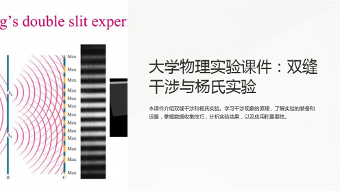
《大学物理实验课件:双缝干涉与杨氏实验》
Use a ruler or caliper to measure the distances involved in the experiment.
Take photos of the interference pattern to aid in data analysis and presentation.
Understand the concept of path difference and its effect on interference fringes.Leabharlann 3 Interference
Equation
Derive the equation for calculating the position of interference fringes.
Wavefront Engineering
Learn how double slit interference is used in various applications, such as wavefront engineering for optics.
Optical Interferometry
Experimental Setup
Understand the components and arrangement required to observe double slit interference.
Observing Interference
Discover how the pattern of bright and dark fringes is formed on a screen.
distance to optimize the
interference pattern.
Rossby波光路追踪V0.6.0用户指南说明书

Package‘raytracing’October14,2022Title Rossby Wave Ray TracingVersion0.6.0Date2022-06-06Description Rossby wave ray paths are traced froma determined source,specified wavenumber,and directionof propagation.``raytracing''also works with a set ofexperiments changing these parameters,making possible theidentification of Rossby wave sources automatically.The theory used here is based on classical studies,such as Hoskins and Karoly(1981)<doi:10.1175/1520-0469(1981)038%3C1179:TSLROA%3E2.0.CO;2>,Karoly(1983)<doi:10.1016/0377-0265(83)90013-1>,Hoskins and Ambrizzi(1993)<doi:10.1175/1520-0469(1993)050%3C1661:RWPOAR%3E2.0.CO;2>,and Yang and Hoskins(1996)<doi:10.1175/1520-0469(1996)053%3C2365:PORWON%3E2.0.CO;2>.License GPL-3Encoding UTF-8LazyData noImports ncdf4,graphics,sf,units,utilsSuggests testthat,covr,lwgeomURL https:///salvatirehbein/raytracing/BugReports https:///salvatirehbein/raytracing/issues/ RoxygenNote7.2.0Depends R(>=3.5.0)NeedsCompilation noAuthor Amanda Rehbein[aut,cre](<https:///0000-0002-8714-7931>), Tercio Ambrizzi[sad],Sergio Ibarra-Espinosa[ctb](<https:///0000-0002-3162-1905>), Lívia Márcia Mosso Dutra[rtm]Maintainer Amanda Rehbein<*********************>1Repository CRANDate/Publication2022-06-0623:30:02UTCR topics documented:betaks (2)betam (4)coastlines (6)Ks (6)Ktotal (7)ray (9)raytracing (11)ray_path (12)ray_source (13)trin (15)wave_arrival (16)ypos (17)Index18 betaks Calculates Beta and KsDescriptionbetaks ingests the time-mean zonal wind(u),transform it in mercator coordinates(um);calculates the meridional gradient of the absolute vorticity(beta)in mercator coordinates(betam);and,finally, calculates stationary wavenumber(Ks)in mercator coordinates(ksm)(see:Hoskins and Ambrizzi, 1993).betaks returns the um,betam,and lat,for being ingested in ray or ray_source.Usagebetaks(u,lat="lat",lon="lon",uname="uwnd",ofile,a=6371000,plots=FALSE,show.warnings=FALSE)Argumentsu String indicating the input datafilename.Thefile to be passed consists in a netCDFfile with only time-mean zonal wind at one pressure level,latitude inascending order(not a requisite),and longitude from0to360.It is requiredthat the read dimensions express longitude(in rows)x latitude(in columns).ualso can be a numerical matrix with time-mean zonal wind at one pressure level,latitude in ascending order(not a requisite),and longitude from0to360.Itis required that the read dimensions express longitude(in rows)x latitude(incolumns).lat String indicating the name of the latitudefield.If u is a matrix,lat must be numeric.lon String indicating the name of the longitudefield.If u is a matrix,lon must be numeric from0to360.uname String indicating the variable namefieldofile String indicating thefile name for store output data.If missing,will not return a netCDFfilea Numeric indicating the Earth’s radio(m)plots Logical,if TRUE will producefilled.countour plotsshow.warnings Logical,if TRUE will warns about NaNs in sqrt(<0)Valuelist with one vector(lat)and3matrices(um,betam,and ksm)Examples{#u is NetCDF and lat and lon charactersinput<-system.file("extdata","uwnd.mon.mean_200hPa_2014JFM.nc",package="raytracing")b<-betaks(u=input,plots=TRUE)b$ksm[]<-ifelse(b$ksm[]>=16|b$ksm[]<=0,NA,b$ksm[])cores<-c("#ff0000","#ff5a00","#ff9a00","#ffce00","#f0ff00")graphics::filled.contour(b$ksm[,-c(1:5,69:73)],col=rev(colorRampPalette(cores,bias=0.5)(20)),main="Ks")#u,lat and lon as numericinput<-system.file("extdata","uwnd.mon.mean_200hPa_2014JFM.bin",package="raytracing")u<-readBin(input,what=numeric(),size=4,n=144*73*4)lat<-seq(-90,90,2.5)lon<-seq(-180,180-1,2.5)u<-matrix(u,nrow=length(lon),ncol=length(lat))graphics::filled.contour(u,main="Zonal Wind Speed[m/s]")b<-betaks(u,lat,lon)b$ksm[]<-ifelse(b$ksm[]>=16|b$ksm[]<=0,NA,b$ksm[])cores<-c("#ff0000","#ff5a00","#ff9a00","#ffce00","#f0ff00")graphics::filled.contour(b$ksm[,-c(1:5,69:73)],col=rev(colorRampPalette(cores,bias=0.5)(20)),main="Ks")}betam Calculates Meridional Gradient of the Absolute Vorticity(beta)inmercator coordinates(betam)Descriptionbetam ingests the time-mean zonal wind(u),transform it in mercator coordinates(um)and then calculates the meridional gradient of the absolute vorticity(beta)in mercator coordinates(betam) using equation Karoly(1983).betam returns a list with the u,betam,and lat for being ingested in Ktotal,Ks,ray or ray_source.Usagebetam(u,lat="lat",lon="lon",uname="uwnd",ofile,a=6371000,plots=FALSE,show.warnings=FALSE)Argumentsu String indicating the input datafilename.Thefile to be passed consists in a netCDFfile with only time-mean zonal wind at one pressure level,latitude inascending order(not a requisite),and longitude from0to360.It is requiredthat the read dimensions express longitude(in rows)x latitude(in columns).ualso can be a numerical matrix with time-mean zonal wind at one pressure level,latitude in ascending order(not a requisite),and longitude from0to360.Itis required that the read dimensions express longitude(in rows)x latitude(incolumns).lat String indicating the name of the latitudefield.If u is a matrix,lat must be numeric.lon String indicating the name of the longitudefield.If u is a matrix,lon must be numeric from0to360.uname String indicating the variable namefieldofile String indicating thefile name for store output data.If missing,it will not returna netCDFfilea Numeric indicating the Earth’s radio(m)plots Logical,if TRUE will producefilled.countour plotsshow.warnings Logical,if TRUE will warns about NaNs in sqrt(<0)Valuelist with one vector(lat)and2matrices(u and betam)Examples{#u is NetCDF and lat and lon charactersinput<-system.file("extdata","uwnd.mon.mean_200hPa_2014JFM.nc",package="raytracing")b<-betam(u=input,plots=TRUE)cores<-c("#ff0000","#ff5a00","#ff9a00","#ffce00","#f0ff00")graphics::filled.contour(b$betam/10e-12,zlim=c(0,11),col=rev(colorRampPalette(cores)(24)),main="Beta Mercator(*10e-11)")#u,lat and lon as numericinput<-system.file("extdata","uwnd.mon.mean_200hPa_2014JFM.bin",package="raytracing")u<-readBin(input,what=numeric(),size=4,n=144*73*4)lat<-seq(-90,90,2.5)lon<-seq(-180,180-1,2.5)u<-matrix(u,nrow=length(lon),ncol=length(lat))graphics::filled.contour(u,main="Zonal Wind Speed[m/s]")}6Ks coastlines CoastlinesDescriptionGeometry of coastlines,class"sfc_MULTILINESTRING""sfc"from the package"sf"Usagedata(coastlines)FormatGeometry of coastlines"sfc_MULTILINESTRING"MULTILINESTRING Geometry of coastlines"sfc_MULTILINESTRING"data(coastlines)Sourcehttps:///downloads/10m-physical-vectors/10m-coastline/ Ks Calculates Total Wavenumber for Stationary Rossby Waves(Ks)DescriptionKs ingests the time-mean zonal wind(u)and calculates the Total Wavenumber for Stationary Rossby waves(Ks)in mercator coordinates(see:Hoskins and Ambrizzi,1993).Stationary Rossby waves are found when zonal wave number(k)is constant along the trajectory,which leads to wave fre-quency(omega)zero.In this code Ks is used to distinguish the total wavenumber for Stationary Rossby Waves(Ks)from the total wavenumber for Rossby waves(K),and zonal wave number(k).Ks returns a list with Ks in mercator coordinates(ksm).UsageKs(u,lat="lat",lon="lon",uname="uwnd",ofile,a=6371000,plots=FALSE,show.warnings=FALSE)Argumentsu String indicating the input datafilename.Thefile to be passed consists in a netCDFfile with only time-mean zonal wind at one pressure level,latitude inascending order(not a requisite),and longitude from0to360.It is requiredthat the read dimensions express longitude(in rows)x latitude(in columns).ualso can be a numerical matrix with time-mean zonal wind at one pressure level,latitude in ascending order(not a requisite),and longitude from0to360.Itis required that the read dimensions express longitude(in rows)x latitude(incolumns).lat String indicating the name of the latitudefield.If u is a matrix,lat must be numeric.lon String indicating the name of the longitudefield.If u is a matrix,lon must be numeric from0to360.uname String indicating the variable namefieldofile String indicating thefile name for store output data.If missing,will not return a netCDFfilea Numeric indicating the Earth’s radio(m)plots Logical,if TRUE will producefilled.countour plotsshow.warnings Logical,if TRUE will warns about NaNs in sqrt(<0)Valuelist with one vector(lat)and1matrix(Ksm)Examples{#u is NetCDF and lat and lon charactersinput<-system.file("extdata","uwnd.mon.mean_200hPa_2014JFM.nc",package="raytracing")Ks<-Ks(u=input,plots=TRUE)Ks$ksm[]<-ifelse(Ks$ksm[]>=16|Ks$ksm[]<=0,NA,Ks$ksm[])cores<-c("#ff0000","#ff5a00","#ff9a00","#ffce00","#f0ff00")graphics::filled.contour(Ks$ksm[,-c(1:5,69:73)],col=rev(colorRampPalette(cores,bias=0.5)(20)),main="Ks")}Ktotal Calculates Total Wavenumber for Rossby Waves(K)DescriptionKtotal ingests the time-mean zonal wind(u)and calculates the Rossby wavenumber(K)(non-zero frequency waves)in mercator coordinates.In this code Ktotal is used to distinguish the total wavenumber(K)from zonal wave number(k).For stationary Rossby Waves,please see Ks.Ktotal returns a list with K in mercator coordinates(ktotal_m).UsageKtotal(u,lat="lat",lon="lon",uname="uwnd",cx,ofile,a=6371000,plots=FALSE,show.warnings=FALSE)Argumentsu String indicating the input datafilename.Thefile to be passed consists in a netCDFfile with only time-mean zonal wind at one pressure level,latitude inascending order(not a requisite),and longitude from0to360.It is requiredthat the read dimensions express longitude(in rows)x latitude(in columns).ualso can be a numerical matrix with time-mean zonal wind at one pressure level,latitude in ascending order(not a requisite),and longitude from0to360.Itis required that the read dimensions express longitude(in rows)x latitude(incolumns).lat String indicating the name of the latitudefield.If u is a matrix,lat must be numericlon String indicating the name of the longitudefield.If u is a matrix,lon must be numeric from0to360.uname String indicating the variable namefieldcx numeric.Indicates the zonal phase speed.Must be greater than zero.For cx equal to zero(stationary waves see Ks)ofile String indicating thefile name for store output data.If missing,will not return a netCDFfilea Numeric indicating the Earth’s radio(m)plots Logical,if TRUE will producefilled.countour plotsshow.warnings Logical,if TRUE will warns about NaNs in sqrt(<0)Valuelist with one vector(lat)and1matrix(ktotal_m)ray9 Examples{#u is NetCDF and lat and lon charactersinput<-system.file("extdata","uwnd.mon.mean_200hPa_2014JFM.nc",package="raytracing")Ktotal<-Ktotal(u=input,cx=6,plots=TRUE)cores<-c("#ff0000","#ff5a00","#ff9a00","#ffce00","#f0ff00")graphics::filled.contour(Ktotal$ktotal_m[,-c(1:5,69:73)],col=rev(colorRampPalette(cores,bias=0.5)(20)),main="K")}ray Calculates the Rossby waves ray pathsDescriptionray returns the Rossby wave ray paths(lat/lon)triggered from one initial source/position(x0,y0), one total wavenumber(K),and one direction set up when invoking the function.ray must ingest the meridional gradient of the absolute vorticity in mercator coordinates betam,the zonal mean wind u,and the latitude vector(lat).Those variables can be obtained(recommended)using betaks function.The zonal means of the basic state will be calculated along the ray program,as well as the conversion to mercator coordinates of u.Usageray(betam,u,lat,x0,y0,K,dt,itime,direction,cx=0,interpolation="trin",tl=1,a=6371000,verbose=FALSE,ofile)10rayArgumentsbetam matrix(longitude=rows x latitude from minor to major=columns)obtained with betaks.betam is the meridional gradient of the absolute vorticity in mer-cator coordinatesu matrix(longitude=rows x latitude from minor to major=columns)obtained with betaks.Is the zonal wind speed in the appropriate format for the ray.Itwill be converted in mercator coordinates inside the raylat Numeric vector of latitudes from minor to major(ex:-90to90).Obtained with betaksx0Numeric value.Initial longitude(choose between-180to180)y0Numeric value.Initial latitudeK Numeric value;Total Rossby wavenumberdt Numeric value;Timestep for integration(hours)itime Numeric value;total integration time.For instance,10days times4times per daydirection Numeric value(possibilities:1or-1)It controls the wave displacement:If1, the wave goes to the north of the source;If-1,the wave goes to the south of thesource.cx numeric.Indicates the zonal phase speed.The program is designed for eastward propagation(cx>0)and stationary waves(cx=0,the default).interpolation Character.Set the interpolation method to be used:trin or ypostl Numeric value;Turning latitude.Do not change this!It will always start with a positive tl(1)and automatically change to negative(-1)after the turning latitudea Earth’s radio(m)verbose Boolean;if TRUE(default)return messages during compilationofile Character;Outputfile name with.csv extension,for instance,"/user/ray.csv"Valuesf data.frameSee Alsoray_sourceExamples{#For Coelho et al.(2015):input<-system.file("extdata","uwnd.mon.mean_200hPa_2014JFM.nc",package="raytracing")b<-betaks(u=input)rt<-ray(betam=b$betam,u=b$u,raytracing11 lat=b$lat,K=3,itime=10*4,x0=-130,y0=-30,dt=6,direction=-1,cx=0,interpolation="trin")rp<-ray_path(rt$lon,rt$lat)plot(rp,main="Coelho et al.(2015):JFM/2014",axes=TRUE,cex=2,graticule=TRUE)}raytracing raytracing:Rossby Wave Ray TracingDescriptionRossby wave ray paths are traced from a determined source,specified wavenumber,and direction ofpropagation.’raytracing’also works with a set of experiments changing these parameters,makingpossible the identification of Rossby wave sources automatically.Authors•Amanda Rehbein(ORCID:https:///0000-0002-8714-7931-mantainer:*********************)•Tercio Ambrizzi(ORCID:https:///0000-0001-8796-7326)•Sergio Ibarra Espinosa(ORCID:https:///0000-0002-3162-1905)•Livia Marcia Mosso Dutra(ORCID:https:///0000-0002-1349-7138)ReferencesHoskins,B.J.,&Ambrizzi,T.(1993).Rossby wave propagation on a realistic longitudinallyvaryingflow.Journal of the Atmospheric Sciences,50(12),1661-1671.Hoskins,B.J.,&Karoly,D.J.(1981).The steady linear response of a spherical atmosphere tothermal and orographic forcing.Journal of the Atmospheric Sciences,38(6),1179-1196.Karoly,D.J.(1983).Rossby wave propagation in a barotropic atmosphere.Dynamics of Atmo-spheres and Oceans,7(2),111-125.Yang,G.Y.,&Hoskins,B.J.(1996).Propagation of Rossby waves of nonzero frequency.Journalof the atmospheric sciences,53(16),2365-2378.12ray_path ray_path Calculate the ray paths/segment of great circlesDescriptionThis function calculates the segments great circles using the(lat,lon)coordinates obtained with ray or ray_source.It returns a LINESTRING geometry that is ready for plot.Usageray_path(x,y)Argumentsx vector with the longitude obtained with ray or ray_sourcey vector with the latitude obtained with ray or ray_sourceValuesfc_LINESTRING sfcExamples{#Coelho et al.(2015):input<-system.file("extdata","uwnd.mon.mean_200hPa_2014JFM.nc",package="raytracing")b<-betaks(u=input)rt<-ray(betam=b$betam,u=b$u,lat=b$lat,K=3,itime=30,x0=-135,y0=-30,dt=6,direction=-1)rp<-ray_path(x=rt$lon,y=rt$lat)plot(rp,axes=TRUE,graticule=TRUE)}ray_source Calculate the Rossby waves ray paths over a source regionDescriptionray_source returns the Rossby wave ray paths(lat/lon)triggered from one or more initial source/position (x0,y0),one or more total wavenumber(K),and one or more direction set up when invoking the function.ray_source must ingest the meridional gradient of the absolute vorticity in mercator coordinates betam,the zonal mean wind u,and the latitude vector(lat).Those variables can be obtained(recommended)using betaks function.The zonal means of the basic state will be calcu-lated along the ray program,as well as the conversion to mercator coordinates of u.The resultant output is a spatial feature object from a combination of initial andfinal positions/sources,total wavenumbers(K),and directions.Usageray_source(betam,u,lat,x0,y0,K,cx,dt,itime,direction,interpolation="trin",tl=1,a=6371000,verbose=FALSE,ofile)Argumentsbetam matrix(longitude=rows x latitude from minor to major=columns)obtainedwith betaks.betam is the meridional gradient of the absolute vorticity in mer-cator coordinatesu matrix(longitude=rows x latitude from minor to major=columns)obtainedwith betaks.Is the zonal wind speed in the appropriate format for the ray.Itwill be converted in mercator coordinates inside the raylat Numeric vector of latitudes from minor to major(ex:-90to90).Obtained withbetaksx0Vector with the initial longitudes(choose between-180to180)y0Vector with the initial latitudesK Vector;Total Rossby wavenumbercx numeric.Indicates the zonal phase speed.The program is designed for eastward propagation(cx>0)and stationary waves(cx=0,the default).dt Numeric value;Timestep for integration(hours)itime Numeric value;total integration time.For instance,10days times4times per daydirection Vector with two possibilities:1or-1It controls the wave displacement:If1, the wave goes to the north of the source;If-1,the wave goes to the south of thesource.interpolation Character.Set the interpolation method to be used:trin or ypostl Numeric value;Turning latitude.Do not change this!It will always start with a positive tl(1)and automatically change to negative(-1)after the turning latitude.a Earth’s radio(m)verbose Boolean;if TRUE(default)return messages during compilationofile Character;Outputfile name with.csv extension,for instance,"/user/ray.csv"Valuesf data.frameExamples##Not run:#do not runinput<-system.file("extdata","uwnd.mon.mean_200hPa_2014JFM.nc",package="raytracing")b<-betaks(u=input)rt<-ray_source(betam=b$betam,u=b$u,lat=b$lat,K=3,itime=10*4,cx=0,x0=-c(130,135),y0=-30,dt=6,direction=-1,interpolation="trin")#Plot:data(coastlines)plot(coastlines,reset=FALSE,axes=TRUE,graticule=TRUE,col="grey",main="Coelho et al.(2015):JFM/2014")trin15 plot(rt[sf::st_is(rt,"LINESTRING"),]["lon_ini"],add=TRUE,lwd=2,pal=colorRampPalette(c("black","blue")))##End(Not run)trin Performs trigonometric interpolationDescriptionThis function performs trigonometric interpolation for the passed basic state variable and the re-quested latitudeUsagetrin(y,yk,mercator=FALSE)Argumentsy Numeric.The latitude where the interpolation is requiredyk Numeric vector of the data to be interpolated.For instance,umz or betammercator Logical.Is it require to transform thefinal data in mercator coordinates?Default is FALSE.ValueNumeric valueNoteThis function is an alternative to ypos and is more accurateSee Alsoypos ray ray_sourceOther Interpolation:ypos()Examples{input<-system.file("extdata","uwnd.mon.mean_200hPa_2014JFM.nc",package="raytracing")b<-betaks(u=input)umz<-rev(colMeans(b$u,na.rm=TRUE))*cos(rev(b$lat)*pi/180)betamz<-rev(colMeans(b$betam,na.rm=TRUE))16wave_arrival y0<--17trin(y=y0,yk=umz)}wave_arrival Filter the ray paths that arrives in an area of interestDescriptionwave_arrival ingests the ray paths tofilter by determined area of interest.Default CRS4326.Usagewave_arrival(x,aoi=NULL,xmin,xmax,ymin,ymax,ofile)Argumentsx sf data.frame object with the LINESTRINGS to befiltered.aoi String giving the path and thefilename of the area of interest.By default is NULL.If no aoi is not provided,the xmin,xmax,ymin,and ymax must beprovided.xmin Numeric.Indicates the western longitude to be used in the range-180to180.xmax Numeric.Indicates the eastern longitude to be used in the range-180to180.ymin Numeric.Indicates the southern longitude to be used in the range-90to90.ymax Numeric.Indicates the northern longitude to be used in the range-90to90.ofile Character;Outputfile name with.csv extension,for instance,"/user/aoi_ray.csv"Valuesf data.frameExamples{}ypos17 ypos Interpolation selecting the nearest neighborDescriptionThis function get the position in a vector of a given latitute y.Usageypos(y,lat,yk,mercator=FALSE)Argumentsy numeric value of one latitudelat numeric vector of latitudes from minor to majoryk numeric vector to be approximatedmercator Logical.Is it require to transform thefinal data in mercator coordinates?Default is FALSE.ValueThe position where the latitude y has the minor difference with latSee AlsoOther Interpolation:trin()Examples{input<-system.file("extdata","uwnd.mon.mean_200hPa_2014JFM.nc",package="raytracing")b<-betaks(u=input)ykk<-rev(colMeans(b$betam))ypos(y=-30,lat=seq(90,-90,-2.5),yk=ykk)}Index∗Interpolationtrin,15ypos,17∗datasetscoastlines,6betaks,2,9,10,13betam,4coastlines,6Ks,4,6,8Ktotal,4,7ray,2,4,9,15ray_path,12ray_source,2,4,10,13,15raytracing,11trin,10,14,15,17wave_arrival,16ypos,10,14,15,1718。
基于几何光学近似迭代的多重散射波面分析
2021 年 3 月第 44 卷 第 2 期湖南师范大学自然科学学报Journal of Natural Science of Hunan Normal University Vel.54 No.2Mar., 2021DOI : 10.7612/j5ssn.2096W2'l .2021.02.012基于几何光学近似迭代的多重散射波面分析彭梓齐",杨江河(湖南文理学院数理学院,中国常德415000)摘要为了解析环状光在散射媒质中的传播特性,本文提出了以几何光学近似为基础的波面分析法来进行分析。
该方法主要以几何光学近似法为工具计算散射粒子的前方散射光,并运用迭代计算的方式实现多重散射模 型的波面分析。
本文运用该方法计算了散射媒质中的透射率以及环状光在散射媒质中的散射强度波形。
计算结 果与实验结果一致,散射媒质在特定的距离以及浓度下,环状光的散射波面中心会出现干涉波峰。
关键词几何光学近似;多重散射;前方散射;干涉中图分类号 O436.1 文献标识码 A 文章编号 2096-5281( 2021) 02-0087-08Wavefrant Analysis of Multiglo Scattering Based onGeometric Optics AppraximationPL#$ Zi-/i ** , B4NG 8a'g-0&收稿日期:2020-07-08基金项目:国家自然科学基金资助项目(U14311⑵;湖南省自然科学基金资助项目(2020JJ5396);湖南省2018年普通高校教育教学改革研究项目(湘教通[2018]436号);湖南文理学院博士启动项目(E07018021)* 通信作者,E-mail : pengzq@ (Colleac of Mathematics and Physics , Hunan University of Arts and Science , Changde 415000, China )Abstracr Tv analyzv thv charycte/stics of annular beam propagation in random media , wv proposed a new wavefront analysis method based on geometWc optics approximation. In this algorithm , wv adopted a simplified gev- metic optics approximation and iterative calculation based on forsard scatte/ng and simulated thv attenuation and thv scatw/ng waveform of thv annular beam in random media. An inWr^ered peak was obtained at thv optical axis with a coiain propagation distance and media concentrations , which is consistent with thv expe/mentat results.Key wordt geometWc optics approximation ; multiplv scytte/ng ; forsard scytte/ng ; inte/erenco光学遥感作为成熟的测量技术在工业、医疗、环保等领域得到了广泛应用W 在光学遥感应用中,光 在媒质中的传播效率是影响光学测量结果与精度的一项重要参数。