Correlations between p_T and Multiplicity in a Single BFKL Pomeron
grey correlation analysis
Grey Correlation AnalysisIntroductionGrey correlation analysis is a statistical method used to measure the correlation between two or more variables when the data is limited or uncertain. It was developed by Deng Julong in China in the 1980s and has since been widely applied in various fields including finance, economics, engineering, and social sciences.Grey correlation analysis is particularly useful when dealing with incomplete or uncertain data. It can provide valuable insights and helpin decision-making processes when traditional correlation analysis methods may not be applicable.Principles of Grey Correlation AnalysisGrey correlation analysis is based on the principles of grey system theory, which aims to study systems with limited information and uncertain data. The method involves four main steps:1.Data Organization: The first step in grey correlation analysis isto organize the available data. This may involve collecting datafrom various sources and arranging it in a systematic manner.2.Data Comparison: Once the data is organized, the next step is tocompare the different variables or factors under consideration.This can be done using various statistical measures such as mean,range, and standard deviation.3.Grey Correlation Coefficient Calculation: The grey correlationcoefficient is calculated to measure the correlation between thevariables. It is a value between 0 and 1, where a higher valueindicates a stronger correlation. The grey correlation coefficient takes into account the uncertainties and variations in the data.4.Grey Correlation Analysis: Finally, the grey correlation analysisis performed to determine the relationships between the variables.This can help in identifying the most influential factors andmaking predictions or forecasts based on the available data.Applications of Grey Correlation AnalysisGrey correlation analysis has been widely used in various fields for different purposes. Some of the applications include:1. Financial AnalysisGrey correlation analysis has been applied in financial analysis to study the relationships between different financial indicators. It can help in identifying the key factors influencing the financial performance of companies or investment portfolios. For example, it can be used to analyze the correlation between stock prices and economic indicators such as inflation rates or interest rates.2. Engineering DesignIn engineering design, grey correlation analysis can be used to evaluate the relationship between various design parameters and the performance of a system or product. It can help in optimizing the design process by identifying the most critical factors and their impact on the overall performance. For example, it can be used to analyze the correlation between different manufacturing parameters and the strength of a material.3. Economic ForecastingGrey correlation analysis has also been used in economic forecasting to predict future trends based on historical data. It can help in identifying the key factors influencing economic growth or decline and making accurate predictions. For example, it can be used to analyze the correlation between GDP growth and factors such as consumer spending, investment, and government policies.4. Social SciencesIn social sciences, grey correlation analysis can be used to study the relationships between different social or demographic variables. It can help in understanding the factors influencing social phenomena and making informed policy decisions. For example, it can be used to analyze the correlation between education levels, income levels, and crime rates in a specific region.Advantages and LimitationsGrey correlation analysis has several advantages over traditional correlation analysis methods. Some of the advantages include:•Suitable for limited or uncertain data: Grey correlation analysis can handle situations where the data is incomplete or uncertain,making it useful in real-world applications.•Provides insights in complex systems: Grey correlation analysis can provide valuable insights in complex systems where traditional correlation analysis methods may not be effective.•Helps in decision-making: Grey correlation analysis can help in decision-making processes by identifying the most influentialfactors and their impact on the outcomes.However, grey correlation analysis also has some limitations. These include:•Subject to data quality: The accuracy and reliability of the results obtained through grey correlation analysis are highlydependent on the quality of the data used.•Limited to linear relationships: Grey correlation analysis assumesa linear relationship between the variables under consideration.It may not be suitable for analyzing non-linear relationships.•Interpretation challenges: Interpreting the results of greycorrelation analysis can be challenging due to the complexity ofthe method and the uncertainties involved.ConclusionGrey correlation analysis is a valuable statistical method for measuring the correlation between variables when data is limited or uncertain. It has been widely applied in various fields and has provided valuable insights in complex systems. However, it is important to consider the limitations and challenges associated with grey correlation analysis when using it for decision-making processes. Overall, grey correlation analysis is a useful tool that complements traditional correlation analysis methods and helps in addressing real-world challenges.。
Correlation

CorrelationXu JiajinNational Research Center for Foreign Language Education Beijing Foreign Studies University2Key points•Why correlation?•What is correlation analysis about?•How to make a correlation analysis?–Case studiesWhy Correlation?4Three things that stats can do •1.Summarizing univariate data •2.Testing the significance of differences •3.Exploring relationships b/t variables5Three things that stats can do •1.Summarizing univariate data •2.Testing the significance of differences •3.Exploring relationships b/t variables6探究事物之间的关联•植物的生长是否浇水的多少有关系,有多大关系•足球成绩好坏是否与身体(体质、人种)有关?•兴趣高、成绩好•元认知策略使用越多,学习进步越快•学好统计学有利于身体健康Key ides of correlationanalysis8•Correlation: co ‐relation . The co ‐relation is represented by a ‘correlation coefficient , r .•The range of the coefficient: ‐1to 1.•Three critical values: ‐1, 0and 1.Strength of correlationPositive correlation Strength of correlation Direction of correlationDirection of correlation Positive correlationDirection of correlation•Less Negative correlation12Two main types of correlation•Pearson : standard type, suitable for interval data (e.g. score, freq.)•Pearson r coefficient•Spearman : suitable for ordinal/rank data•Spearman rho coefficient13Significance•Similar to t ‐test and ANOVA statistics, the correlation coefficients need to be statistically significant.< .05Sig./P 值/alpha (α)值Coefficient of Determination r Ær2Æ% of variance explained15Coefficient of Determination •The squared correlation coefficient is called the coefficient of determination .•Multiplied by 100, this proportion of variance indicates the percentage of variance that is accounted for.•Correlation coefficients of .30 account for about 9% of the variance. Correlation of .70 explains about 49% of variance.Effect sizeCase Study 1Is connector use by Chinese EFL learners correlated with theirwriting quality?SPSS ProceduresAnalyze‐Correlate‐Bivariate1921Reporting correlations•In correlation tables/matrices •Embedded in textCorrelation tablesCorrelation tables(Dörnyei2007: 227)2324Embedded in text •As one would expect from the extensive literature documenting the benefits of intrinsic motivation, there was a significant positive correlation between overall GPA and intrinsic motivation (r = .34, p < .oo1).(Dörnyei 2007: 227)Practice: CET4 and CET6 Correlational analysisHomework英语成绩是否与语文成绩有相关性?28Wrap Up & Look Forward •Correlation coefficients provide a way to determine the strength & the direction of the relationship b/t two variables.•This index does not ... demonstrate a causal association b/t two variables.29Wrap Up & Look Forward •The coefficient of determination determines how much variance in one variable is explained by another variable.•Correlation coefficients are the precursors to the more sophisticated statistics involved in multiple regression (Urdan 2005: 87).30Thank you32。
A Reconsideration of Testing for Competence Rather Than for Intelligence
A Reconsideration of Testing for CompetenceRather Than for IntelligenceGerald V. Barrett and Robert L. DepinetThe University of AkronCorrespondence concerning this article should be addressed to GeraldV. Barrett, Department of Psychology, The University of Akron, BuchtelCollege of Arts and Sciences, Akron, OH 44325-4301.October 1991 ° American PsychologistDavid C. McClelland's 1973 article has deeply influenced both professional and public opinion. In it, he presented five major themes: (a) Grades in school did not predict occupational success, (b) intelligence tests and aptitude tests did not predict occupational success or other important life outcomes, (c) tests and academic performance only predicted job performance because of an underlying relationship with social status, (d) such tests were unfair to minorities, and (e) "competencies" would be better able to predict important behaviors than would more traditional tests. Despite the pervasive influence of these assertions, this review of the literature showed only limited support for these claims.In 1973, David C. McClelland's lead article in the American Psychologist profoundly affected both the field of psychology and popular opinion. This article was designed to "review skeptically the main lines of evidence for the validity of intelligence and aptitude tests and to draw some inferences from this review as to new lines that testing might take in the future" (p. 1). The main themes he endorsed and continues to promote (e.g., Klemp & McClelland, 1986) have been published widely in newspapers, magazines, and popular books as well as psychology textbooks. Belief in these views, however, has become so widespread that often they are presented as com- mon knowledge (e.g., Feldman, 1990).Table 1 reviews a number of works that cited McClelland (1973) and shows that the impact of McClelland's article has increased over time. Soon after the article was published, McClelland's views were integrated into introductory psychology textbooks. By the late 1980s, these themes had become part of generally accepted public opinion, with newspaper and magazine writers commonly citing McClelland as an authority on intelligence testing.It was McClelland's (1973) belief that intelligence testing should be replaced by competency-based testing. His argument against intelligence testing rested on the assertion that intelligence tests and aptitude tests have not been shown to be related to important life outcomes because psychologists were unable and unwilling to test this relationship. McClelland argued that intelligence tests have been correlated with each other and with grades in school but not with other life outcomes.McClelland (1973) stated that intellectual ability scores and academic performance were theresult of social status, and he labeled them a sort of game. He asserted that a test must resemble job performance or other criteria to be related to the performance on the criteria. He also claimed that intelligence and aptitude testing were unfair to minorities. He advocated that the profession should focus on what he termed competency testing and criterion sampling, maintaining that intelligence testing and aptitude testing should be discarded.The main points of McClelland's (1973) article can be summarized in the following five themes: (a) Grades in school did not predict occupational success, (b) intelligence tests and aptitude tests did not predict occupational success or other important life outcomes, (c) tests and academic performance only predicted job performance as a result of an underlying relationship to social status, (d) traditional tests were unfair to minorities, and (e) "competencies" would more successfully predict important behaviors than would more traditional tests.In the present article, these themes are examined through a comprehensive review of relevant literature. Although McClelland's (1973) article contained many subthemes, only those themes we believe to be the main issues are addressed here. This does not imply, however, that we agree with any aspects of McClelland's article that are not addressed here.Do Grades Predict Occupational Success?McClelland (1973) claimed that "the games people are required to play on aptitude tests are similar to the games teachers require in the classroom" (p. 1). As evidence, McClelland presented four citations that he interpreted as support for his position, while ignoring disconfirming evidence. He also included his personal experiences at Wesleyan University as evidence, maintaining that "A" students could not be distinguished from barely passing students in later occupational success. This finding differs greatly from that found in a similar, more scientific comparison done by Nicholson (1915) at the same school. Nicholson found that academically exceptional students were much more likely to achieve distinction in later life. The results of Nicholson's study are summarized in Table 2.Table 1 Support for McClelland's (1973) Concepts in Newspapers, Magazines, Popular Books, and TextbooksPublication Author(s) Statement NewspapersNew York Times Goleman (1988) IQ tests severely limited as predictors of job successNew York Times Goleman (1984) Intelligence unrelated to career successPlain Dealer Drexler (1981) Tests unrelated to accomplishments in leadership, arts, science, music, writing, speech, and drama; tests discriminate by culture MagazinesAtlantic MonthlyPsychology TodayPsychology TodayPopular booksMore Like UsWhiz KidsPsychology textsPsychology: An IntroductionIntroduction to PsychologyPsychology: Being HumanPsychologyUnderstanding Human BehaviorElements of PsychologyEssentials of PsychologyPsychology: An IntroductionIntroductory PsychologyFallows (1985)Goleman (1981)Koenig (1974)Fallows (1989)Machlowitz (1985)Morris (1990)Coon (1986)Rubin & McNeil (1985)Crider, Goethals,Kavanaugh, &Solomon (1983)McConnell (1983)Krech & Crutchfield(1982)Silverman (1979)Mussen &Rosenzweig (1977)Davids & Engen(1975)Promote replacing aptitude tests with competence testsTests and grades are unrelated to career successTests and grades have less value than competence testsTests and grades are useless as predictors of occupational success Bright people do not do better in lifeIQ and grades are unrelated to occupational successIQ does not predict important behaviors or successSuggests replacing IQ tests with competence testsTests are unfair by race and socioeconomic statusAbility is unrelated to career successTests and grades are unrelated to life outcomesTesting results in categorical labelsTest scores are unrelated to job successSuggests replacing IQ tests with competence testsSome limitations do exist when grades are used as predictors. Grades vary greatly among disciplines (Barrett & Alexander, 1989; EUiott & Strenta, 1988; Schoenfeldt & Brush, 1975) as well as among colleges (Barrett & Alexander, 1989; Humphreys, 1988; Nelson, 1975). Because different students usually take different courses, the reliability of grades is relatively low unless a common set of courses is taken (Butler & McCauley, 1987). Despite these shortcomings, a number of meta-analyses have shown that grades do have a small-to-moderate correlation with occupational success (Cohen, 1984; Dye & Reek, 1988, 1989; O'Leary, 1980; Samson, Graue, Weinstein, & Walberg, 1984). Despite an overlap among the data used by these studies and variability among results (r =. 15 to .29), they all reached similar conclusions. A wide variety of measures of occupational success such as salary, promotion rate, and supervisory ratings have been positively related to grade point average.Table 2 Success of Wesleyan GraduatesClasses/academic standing Percentage who achieved distinction in later life1831-1959Valedictorians and salutatorians 49Phi Beta Kappa 31No scholarly distinction 61860-1889Highest honors 47Phi Beta Kappa 31No scholarly distinction 101890-1899Highest honors 60Phi Beta Kappa 30No scholarly distinction 11Note. Adapted from "Success in college and in later life" by F. W. Nicholson,1915, School and Society, 12, p. 229-232. In the public domain.The results of these recta-analyses reflect the diverse individual studies that showed a relationship between academic performance and occupational success. This relationship may have stemmed from underlying associations between academic performance and intellectual ability, motivation (Howard, 1986), and attitudes toward work (Palmer, 1964). Hunter (1983, 1986) supported this possibility by demonstrating through path analysis that higher ability led to increased job knowledge, which in turn led to better job performance. This relationship was true at all educational levels, including medical school graduates, graduate-level MBAs, college graduates in both engineering and liberal arts, technical school graduates, and high school graduates in the United States and in other countries, such as Sweden (Husen, 1969). The correlations between grades and occupational success have ranged from .14 to .59. However, some research has indicated that these relationships were underestimated because the range onthe predictor grades was restricted (Dye & Reck, 1989; Elliott & Strenta, 1988). Even when limitations are considered, both meta-analyses and diverse individual studies showed grades as predictors of occupational success.Do Intelligence Tests and Aptitude Tests Relate to Job Success or Other Life Outcomes?Thorndike and Hagen's (1959) study was McClelland's (1973) central evidence that aptitude tests did not predict occupational success. The Thorndike and Hagen study involved more than 12,000 correlations between aptitude tests and various measures of occupational success for more than 10,000 individuals. They concluded that the number of significant correlations did not exceed the number that would be expected by chance. From these results, MeClelland concluded that "in other words, the tests were invalid" (p. 3).This characterization of the research by Thorndike and Hagen (1959) has often been quoted as proof that aptitude tests cannot predict job success (Haney, 1982; Nairn, 1980). However, McClelland (1973) did not address some extremely important points.Perhaps the most basic point overlooked was that aptitude tests did, in fact, predict success for those professionals for whom they were designed, namely, pilots and navigators. The test battery consisted of dial and table reading, speed of identification, two-hand coordination, complex coordination, rotary pursuit, finger dexterity, aiming stress, discrimination in reaction time, reading comprehension, mathematics, numerical operations, and mechanical principles (Dubois, 1947). All of these tests were specifically designed to predict success in avionics, and the content of these tests was directly related to that field. The mechanical principles test, for example, asked the direction of the wind as shown by a wind sock.The validity of the test battery was demonstrated during World War II (Dubois, 1947) when an unscreened group was used as part of the validation process. Of those who failed the test battery, only 8.6% subsequently graduated from training (45 of 520), and no one in the lowest stanine (150 subjects) graduated. Conversely, 85% of those in the upper stanines graduated (Dubois, 1947).M eClelland (1973)was concerned that cultural bias was present in aptitude tests. The avionics battery studied by Thorndike and Hagen (1959) was used to predict the success of pilots during World War II (Dubois, 1947) and included West Point cadets, Chinese people, women, and Blacks as subjects. The battery was found valid for all of these groups. This agrees with later findings that, in general, aptitude tests are valid for all groups (Boehm, 1972; Hunter, Sehmidt, & Hunter, 1979; Hunter, Schmidt, & Rauschenberger, 1984).Thorndike and Hagen (1959) surveyed a sample of individuals who had taken the pilot and navigators test battery in 1943. The respondents, who ranged in age from 18 to 26 years at the time of testing, were asked to supply self-report data in seven areas, including monthly income in1955. Validity coefficients were then computed between results on the avionics test battery and self-reported income.This validation procedure contained obvious flaws. The eight-year age range among subjects influenced the job experience of the respondents. Some respondents were well established in their careers. Others were only beginning. Differences in job experience would translate into wide salary differences, even within the same occupation, contaminating the criterion measure.The respondents were in diverse occupations and were dispersed geographically throughout the United States. Even if the avionics test had been appropriate for predicting the success of both an English academic and a physician and even if they were the same ages at the time the salary data were collected, the differences in mean occupational salary would obscure any potential relationship.While McClelland (1973) was claiming that the avionics battery was invalid for predicting occupational success, other researchers using the same data set as Thorndike and Hagen (1959) refined the procedure and obtained additional criterion data in 1969 (Beaton, 1975; Hause, 1972, 1975; Tanbman & Wales, 1973, 1974). These researchers determined that the numerical aptitude factor, derived by factor analysis, was positively related to later income. These studies also showed that this relationship increased over time as the former aviators and navigators matured in their respective occupation. When the data were broken down by occupation, those respondents scoring in the top one tenth in numerical ability earned 30% more than those scoring in the bottom four tenths. When ability was held constant, education was not a significant factor in relation to earnings (Taubman & Wales, 1974).Taubman and Wales (1974) found that those with scores in the top ability level within each educational category (from high school through professional education) had considerably higher salaries than those at the lowest ability level. For individuals with master's degrees, those scoring in the bottom one fifth averaged an annual salary of $14,000, whereas those in the top one fifth averaged $22,200.Comparable results were obtained in a longitudinal study in Sweden over a 26-year period (Husen, 1969). Men included in the group with the highest intellectual ability, when tested at age 10, earned twice the income of those in the lowest category, a practical and significant difference in income. The evidence presented here leads to the inevitable conclusion that intelligence tests and aptitude tests are positively related to job success.Recent EvidenceMany researchers have tested the relationship between cognitive ability and job performance using meta-analytic techniques. Data from approximately 750 studies on the General Aptitude Test Battery (GATB) showed that the test validly predicted job performance for many different occupations (Hartigan & Wigdor, 1989). Hunter and Hunter's ( 1984 ) recta-analysis demonstrated that in entrylevel positions, cognitive ability predicted job performance with an average validityof .53. This study also showed an average correlation of.45 between intellectual ability and job proficiency. Other studies using a number of different measures of job proficiency have found similar relationships to cognitive ability (Distefano & Pryer, 1985; Hunter, 1983, 1986; Pearlman, Schmidt, & Hunter, 1980; Schmidt, Hunter, & Caplan, 1981).McClelland (1973) implied that supervisors' ratings were biased. However, research has shown that the sex and race of either the rater or ratee do not exert important influence on ratings (Pulakos, White, Oppler, & Borman, 1989). More objective criterion measures produced even higher validity coefficients with aptitude test scores. In Nathan and Alexander's (1988) meta-analysis, the criteria of ratings, rankings, work samples, and production quantities all resulted in high test validities. Production quantity and work sample criteria resulted in substantial validity coefficients, negating McClelland's claim that validity coefficients were obtained only by using biased supervisory ratings. In fact, Smither and Reilly (1987) found that the intelligence of the rater was related to the accuracy of job performance ratings.In a study using path analysis, Schmidt, Hunter, and Outerbridge (1986) found that cognitive ability correlated with job knowledge (.46), work samples (.38), and supervisory ratings (. 16). They concluded that cognitive ability led to an increase in job knowledge, a position also supported by Gottfredson (1986).Practical TasksTo support his assertion that intelligence was not appli- cable to employment situations, McClelland (1973) stated that intelligence as measured in aptitude and intelligence testing was not useful in practical, everyday situations. Schaie (1978) explored this theory, describing the issues that must be addressed to attain external validity. He suggested that criteria should include actual real-world tasks. Willis and Schaie (1986) tested this proposition on older adults. Both the individuals tested and the criterion tasks used in the study, such as ability to comprehend the label on a medicine bottle or to understand the yellow pages of the telephone directory, differed substantially from typical academic tasks. According to McClelland's view, a relationship should not exist between mental abilities, such as fluid and crystallized intelligence, and performance on the eight categories of real-life tasks used by Willis and Schaie.This idea was not supported by the study results. An extremely high relationship existed between intelligence and performance on real-life tasks. Intellectual ability accounted for 80% of the variance in task performance (Willis & Schaie, 1986). In a second study, they again found intellectual ability to be related to both selfperceived performance and the ratings assigned by judges for performing a number of practical tasks. These results were replicated on several samples of older adults (Schaie, 1987).Correlations between performance and scores on intelligence and aptitude tests are supported in other, more unstructured and ambiguous situations including business management (Bray & Grant, 1966; Campbell, Dunnette, Lawler, & Weick, 1970; Siegel & Ghiselli, 1971), performance in groups (Mann, 1959), and success in science (Price, 1963). Michell and Lambourne (1979) studied16-year-old students and found that those with higher cognitive ability were better able to answer openended questions. Students with higher cognitive ability were also able to sustain discussion longer, ask more interpretive questions, and achieve a more complex understanding of issues. In addition, intelligence has been shown to be related to musical ability (Lynn & Gault, 1986) and creativity (Cropley & Maslany, 1969; Drevdahl & Cattell, 1958; Hocevar, 1980; MacKinnon, 1962; McDermid, 1965; Richards, Kinney, Benet, & Merzel, 1988). From examining these studies, we find cognitive ability to be positively related to a variety of real-world behaviors.SummaryA review of the relevant literature shows that intelligence tests are valid predictors of job success and other important life outcomes. Cognitive ability is the best predictor of performance in most employment situations (Arvey, 1986; Hunter, 1986), and this relationship remains stable over extended periods of time (Austin & Hanisch, 1990). Using samples of the size usually found in personnel work, Thorndike (1986) concluded that cognitive "g" is the best predictor of job success. Ironically, this was the same author whose earlier study was presented in McClelland's (1973) article as evidence that aptitude tests cannot be used to predict job performance.The evidence from these varied scientific studies leads again and again to the same conclusion: Intelligence and aptitude tests are positively related to job performance.Is There an Artifactual Relationship Between Intellectual Ability and Job Success Based on Social Status?A major part of McClelland's (1973) argument against the use of intelligence or aptitude tests was his claim that "the tests are clearly discriminatory against those who have not been exposed to the culture, entrance to which is guarded by the tests" (13. 7). Available scientific evidence has refuted this contention; IQ is related to occupational success. However, McClelland maintained that "'the correlation between intelligence test scores and job success often may be an artifact, the product of their joint association with class status" (p. 3).Despite the numerous ways of defining socioeconomic status (SES), we will show that occupational success is primarily a result of individual cognitive ability and education, both factors that are relatively independent of social origin. We will also show that the strength of the relationship between IQ and job success is not strongly related to the social prestige of particular careers, regardless of variations between occupations. We agree with Gottfredson (1986) that it is more useful to focus on areas such as individual ability rather than irrelevant SES factors, such as family income, over which individuals have no control.Definition of Socioeconomic StatusMcClelland's (1973) definition of SES differs considerably from those used by other researchers. To McClelland, socioeconomic status belongs to the power elite--those who have credentials, power, pull, opportunities, values, aspirations, money, and material advantages. Some of these factors (e.g., values and aspirations) have been shown to be related to later success (Sewell & Hauser, 1976). They have not been described as socioeconomic status by other researchers, however, because these factors do not belong exclusively to the wealthy (Greenberg & Davidson, 1972).McClelland (1973) also described SES in terms of income. Other researchers in the area (e.g., Scarr & Weinberg, 1978; Sewell & Hauser, 1976) have found in- come to have weak connections with later success, with correlations of only. 17 between the adult's income and the income of his or her parents (Sewell & Hauser, 1976). These findings are consistent with Alwin and Thornton (1984) and Williams (1976), who found correlations between. 12 and .25 between family income and the intelligence of the children. Although variation exists in the correlations found, none of the results supported McClelland's view of strong financial effects.Some variables that have been examined as operational measures of SES include family structure, dwelling conditions, and school attendance record (Greenberg & Davidson, 1972); number of siblings in the family, region of residence, and size of community (Peterson & Karplus, 1981); number of people per room in the home (Greenberg & Davidson, 1972; Herzog, Newcomb, & Cisin, 1972); mother's educational level (Herzog et al., 1972; Peterson & Karplus, 1981; Sewell & Hauser, 1976; Willerman, 1979); father's educational level (Duncan, Featherman, & Duncan, 1972; Peterson & Karplus, 1981; Sewell & Hauser, 1976; Willerman 1979); father's occupation (Duncan et al., 1972; Greenberg & Davidson, 1972; Peterson & Karplus, 1981; Sewell & Hauser, 1976; Willerman, 1979); family income (Peterson & Karplus, 1981; Sewell & Hauser, 1976); and median neighborhood income and educational level (Scarr, 1981). Socioeconomic status has often been operationally defined as a combination of these factors. Because SES has been defined in so many ways, the specific variables explored were theoretically more important and practical than the general term socioeconomic status.Effects of Socioeconomic Status VariablesMeasures described as SES, such as parental education, have been related to children's success (Duncan et al., 1972; Scarr & Weinberg, 1978; Sewell & Hauser, 1976). These factors were most likely proxies for explanatory factors such as orderliness in the home and value placed on education. Studies show that parental background variables make little contribution to the distribution of individuals to occupations, whereas years of education and cognitive ability make a large contribution (Duncan et al., 1972; Gottfredson & Brown, 1981). A well-known longitudinal study (Vaillant, 1977) found that broad measures of SES before an individual's enrollment in college had no relation to outcome variables 30 years later. However, among people of equal ability, the most significant predictor of adult occupational achievement was the parents' attitudetoward school and education (Kraus, 1984).The operational measures of SES that have been found to be important determinants of later outcomes (e.g., values and attitudes) were factors that could be influenced. Even the poorest of families could develop and use these factors to benefit their children (Greenberg & Davidson, 1972). Unfortunately, some families are so destitute that their environment would not even be considered as humane, and this deprivation would have detrimental effects on later accomplishments. For the vast majority of people in all socioeconomic and racial subgroups, however, this is not the case (Scarf, 1981).Education and measured cognitive ability were shown to be more important to later outcomes than were such factors as income. However, the effect of SES on these variables must be examined further.Test performance. Oakland (1983) found that the relationship between IQ scores andachievement test performance was the same across SES levels. A factor analysis of ability measures in different SES groups showed that factor structure was not contingent on SES (Humphreys & Taber, 1973). Spaeth (1976) and Valencia, Henderson, and Rankin (1985) found that the effects of parental SES on a child's IQ score were mediated by family interaction and exposure to stimuli provided by parents. In addition, Spaeth concluded that parental influence was a great deal more important than that of teachers and schools. The effects of the latter were much less personal and direct. He concluded that the direct effect of parental SES on child's IQ was -.03. In related research, SES has not been found to have a significant effect on the IQ scores of adult, adopted twins reared apart (Bouchard, Lykken, McGue, Segal, & Tellegen, 1990).Simple measures of SES did not adequately capture the parts of the environment that produced individual differences, even within families (Mercy & Steelman, 1982; Rowe & Plomin, 1981). Even such simple, specific variables as amount of time spent on homework and amount of time spent watching TV on weekdays were related in the expected direction to performance on academic achievement tests (Keith, Reimers, Fehrmann, Pottehaum, & Aubey, 1986). Ultimately, parents could help children learn to cope with cognitive complexity, an effect independent of SES (Spaeth, 1976).College attendance. Contrary to McClelland's (1973, p. 3) assertion that entrance intoprestigious jobs was based on social background, entrance into higher status jobs has instead been shown to be primarily determined by educational attainment (Alexander & Eckland, 1975; Bajema, 1968; Gottfredson & Brown, 1981; Schiefelbein & Farrell, 1984; Sewell & Hauser, 1976). Therefore, what determines attendance at college is very important.McClelland ( 1973) stated that an individual's socioeconomic class was the primary factor in determining his or her ability to attend college. Research has shown the flaws in this assertion. Although socioeconomic background is associated with college attendance, other factors are。
decay of correlation 数学名词

decay of correlation 数学名词Decay of correlation(相关性的衰减)refers to the decrease in correlation between two variables as the distance between them increases. It is a mathematical concept used to quantify the relationship between two variables across different spatial or temporal distances.1. The decay of correlation between rainfall and crop yield was observed as the distance between the two fields increased.雨量与农作物产量之间的相关性随着两个田地之间的距离增加而减弱。
2. The study analyzed the decay of correlation between interest rates and stock market performance over a one-year timespan.该研究分析了利率和股市表现之间的相关性在一年的时间内是如何衰减的。
3. As the distance between two cities increased, thedecay of correlation between their population sizes became more noticeable.随着两个城市之间的距离增加,它们的人口规模之间的相关性衰减变得更加明显。
4. The researchers used statistical methods to determine the decay of correlation between air pollution andrespiratory diseases in different neighborhoods.研究人员使用统计方法来确定不同社区之间空气污染和呼吸道疾病之间的相关性衰减。
03-06 Correlation

3.6-20
Fitted Line Plot
出现下面的第二张 图面。
3.6-21
Fitted Line Plot
在options中不输入任 何值出现的图面。
} +8
} -8
在options中选择Display Prediction Bands时出现 的图面。
– – – – 杂质导致发泡 杂质导致低收益 增加压力来减少发泡 压力对发泡有反作用,但与收益毫不相干
3.6-17
简单回归
相关告诉我们在两个变量之间有多少线性关联,而回归 则更精确地说明这种关联。 具有一个(或多个)变量的方程的回归结果帮助解释在 另外一个变量中的散布
•
Stat>Regression>Regression
Output
70 Y = 99.1754 - 0.745022X 60 R-Squared = 0.876 50 40 30
Moderate Negative Correlation
110
100
0 10 20 30 40 50 60 70 80
90
Input
Output
80
Weak Negative Correlation
• 我们期望的相关性是什么? • 利用 Stat>Basic Statistics>Correlation 程 序来研究其相关性
– 为什么这个相关不是我们所期待的? – 让我们用分类相关系数画 histogram图
• 利用 Stat>Regression>Fitted Line Plot 程序来研究r-平方
财务风险管理Ch11
14
One-Factor Model continued
If Ui have standard normal distributions we can set
U i ai F 1 ai2 Z i
where the common factor F and the idiosyncratic component Zi have independent standard normal distributions Correlation between Ui and Uj is ai aj
V2 Mapping to U2
V2 0.2 0.4 0.6 0.8
Percentile 8 32 68 92
U2 −1.41 −0.47 0.47 1.41
20
Example of Calculation of Joint Cumulative Distribution
Probability that V1 and V2 are both less than 0.2 is the probability that U1 < −0.84 and U2 < −1.41 When copula correlation is 0.5 this is M( −0.84, −1.41, 0.5) = 0.043 where M is the cumulative distribution function for the bivariate normal distribution
1 w 1 1
.
10
V1 and V2 Bivariate Normal
Conditional on the value of V1, V2 is normal with mean
Correlation dimension A Pivotal statistic for

1
Corresponding author: Michael Small, Department of Mathematics, University of Western Australia, Nedlands, WA 6907, Australia. Tel:+08 9380 3348; Fax: +08 9380 1028; Email: watchman@.au Preprint submitted to Elsevier Preprint 14 October 1997
Correlation dimension: A Pivotal statistic for non-constrained realizations of composite hypotheses in surrogate data analysis.
Michael Small, 1 Kevin Judd
1 Introduction
Surrogate data techniques can be used to test speci c hypotheses, such as: is the data temporally correlated; is the data linearly ltered noise; is the data linearly related? Surrogate data testing consists of comparing the distribution of test statistic values for realizations of a particular class of systems to the test statistic value for a data set. One can then either reject, or fail to reject, the hypothesis that the data came from a system of the assumed form. Ideally one would want to apply surrogate data tests to the data with increasingly broad hypotheses until a hypothesis is su ciently broad that it cannot be rejected. Currently one can only conclude that the data is consistent with a particular type of linear system or something else, that is, a nonlinear system. The purpose of this paper is to begin to make more speci c classi cations within the class of nonlinear systems, for example, a nonlinear system with periodic orbit. For classes of linear systems there are some useful and widely applied algorithms to generate surrogate consistent with three hypotheses 1]. These hypotheses are that: (0) the data is temporally uncorrelated, (1) it is linearly ltered noise, or (2) it is a monotonic nonlinear transformation of linearly ltered noise. The power of these surrogate generation algorithms is that they will generate surrogates that are consistent with the hypothesis being tested and are also similar to the data. When generating nonlinear surrogates we suggest that it may be easier to ensure that the probability distribution of the test statistic is the same for all processes consistent with the hypothesis and choose realizations of any process consistent with that hypothesis as representative. With such a statistic it would be possible to build a nonlinear model (usually with reference to the data) and generate (noise driven) simulations from that model as surrogates.
协方差
1
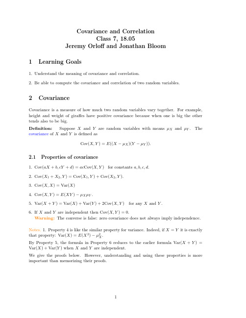
18.05 class 7, Covariance and Correlation, Spring 2014
2
2.2
Sums and integrals for computing covariance
Since covariance is defined as an expected value we compute it in the usual way as a sum or integral. Discrete case: If X and Y have joint pmf p(xi , yj ) then
n m
n
m
p(xi , yj )xi yj − µX µY .CovFra bibliotekX, Y ) =
i=1 j =1
p(xi , yj )(xi − µX )(yj − µY ) =
i=1 j =1
Continuous case: If X and Y have joint pdf f (x, y ) over range [a, b] × [c, d] then
18.05 class 7, Covariance and Correlation, Spring 2014
3
So Cov(XY ) = E (XY ) − µX µY =
5 1 −1= . 4 4 Next we redo the computation of Cov(X, Y ) using the properties of covariance. As usual, let Xi be the result of the ith flip, so Xi ∼ Bernoulli(0.5). We have X = X1 + X2 and Y = X2 + X3 . We know E (Xi ) = 1/2 and Var(Xi ) = 1/4. Therefore using Property 2 of covariance, we have Cov(X, Y ) = Cov(X1 +X2 , X2 +X3 ) = Cov(X1 , X2 )+Cov(X1 , X3 )+Cov(X2 , X2 )+Cov(X2 , X3 ). Since the different tosses are independent we know Cov(X1 , X2 ) = Cov(X1 , X3 ) = Cov(X2 , X3 ) = 0. Looking at the expression for Cov(X, Y ) there is only one non-zero term Cov(X, Y ) = Cov(X2 , X2 ) = Var(X2 ) = 1 . 4
- 1、下载文档前请自行甄别文档内容的完整性,平台不提供额外的编辑、内容补充、找答案等附加服务。
- 2、"仅部分预览"的文档,不可在线预览部分如存在完整性等问题,可反馈申请退款(可完整预览的文档不适用该条件!)。
- 3、如文档侵犯您的权益,请联系客服反馈,我们会尽快为您处理(人工客服工作时间:9:00-18:30)。
a rXiv:h ep-ph/212185v113Dec22February 1,200820:0WSPC/Trim Size:9in x 6in for Proceedings contribution4CORRELATIONS BETWEEN <p T >AND MULTIPLICITY IN A SINGLE BFKL POMERON ∗†M.A.BRAUN Dept.High-Energy Physics St.Petersburg State University 198504St.Petersburg,Russia E-mail:Braun1@pobox.spbu.ru C.MERINO AND G.RODRIGUEZ Department of Particle Physics,Facultade de F´ısica,Universidade de Santiago de Compostela,Campus Universitario s/n,Santiago de Compostela,Galice,Spain E-mail:Merino@c.es E-mail:Grod@c.es Strong correlations are obtained between the number and the average transverse momentum of jets emitted by the exchange of a single BFKL Pomeron.1.IntroductionStrong correlations are observed experimentally between the average p T and multiplicities of particles produced in high-energy hadronic collisions[1].Average p T grows with multiplicity.To interpret this fact it is tacitly assumed that with only one hard collision there are no correlations be-tween <p T >and multiplicity.Theoretically this assumption can only be tested within the Balitskii-Fadin-Kuraev-Lipatov (BFKL)dynamics,which presents a detailed description of particle (actually jet)production at high energies under certain simplifying assumptions (a fixed small coupling con-stant).The present calculation is aimed to see if there exist correlations between <p T >and the number of produced jets in the hard PomeronFebruary1,200820:0WSPC/Trim Size:9in x6in for Proceedings contribution42described by the BFKL chain of interacting reggeized gluons[2].We limitourselves to the leading order BFKL model.2.The FormalismThe BFKL equation for the amputated BFKL amplitude,f(y,k),when yis the rapidity and k is the two-dimensional transverse momentum of thevirtual(Reggeized)gluon,may be written in the formf(y,k)=f(0)(y,k)+¯αs y0dy1 d2k1k21f(y1,k1)−f(y,k)θ(k2−q2) ,(1)where¯αs=3αs/πand q=k−k1is the transverse momentum of theemitted(real)gluon.Defining as an observable jet a real gluon with q2≥µ2,one splits the integration over momenta and thus the integration kernel in(1)into twoparts,a resolved one,K R,corresponding to emitted gluons with q2>µ2,and an unresolved one,K UV,which combines emission of gluons withq2<µ2and the subtraction term in(1).Exclusive probabilities to pro-duce n jets are obtained by introducing n operators K R between the Greenfunctions of the BFKL equations with kernel K UV[3].If one presents thefull gluon distribution f as a sum of contributions f n from the productionof n jets then one gets a recursive relationf n(y)= y0dy1K(y−y1)f n−1(y1),(2)where K(y)is an y-dependent operator in the transverse momentum spaceK(y)=e yK UV K R.(3) Eq.(2)allows one to successively calculate the relative probabilities toproduce n=0,1,2,...jets starting from the no-jet contribution.The exclusive physical probabilities to observe n jets are obtained by convoluting f n with the gluon distribution in the projectile(the projectileimpact factor).Both the impact factors of the target and of the projectileshould vanish as k→0.3.The CalculationWe are interested in the average values of<q>n in the observed jets,provided their number n isfixed.The momentum k which serves as anargument of f(y,k)refers to the virtual gluon,and not to the emitted one,February1,200820:0WSPC/Trim Size:9in x6in for Proceedings contribution43 whose momentum q is hidden inside the kernel K R.Therefore tofind anaverage of any quantityφ(q)depending on the emitted real jet momentum,one has to introduce the functionφ(q)into the integral defining K R,thuschanging the kernel K R to the kernel K av:K av f (k)=¯αs k2 d2k1(dk2/k4)h(k)g n(y,k)nFebruary 1,200820:0WSPC/Trim Size:9in x 6in for Proceedings contribution444.The ResultsWe defined our jets by taking µ=2GeV/c.As for the cutoffs,we used1GeV/c <k 1<100GeV/c,(9)and we used a simplified expression for the virtual photon impact factor,independent of rapidity [2].We have calculated the functions f n and g n from Eqs.(2)and (8)upto n =5and y =15.Following [3]we have used the expansion in NChebyshev polynomials to discretize the kernels in a simple way.In Figure 1we present the averages <q >n for n =1−5and x =e −y =3.10−7−0.1,for the γ∗-hadron collisions (DIS)atQ 2=100(GeV/c)2.468101214<p _T>_nGe V/cxDIS, Q^2=100 (GeV/c)^2Figure 1.Average <p T >n for a fixed number n of jets produced in γ∗-hadron colli-sions,as a function of x at Q 2=100(GeV/c)2.Curves from bottom to top correspondto n =1,2,...5.As one observes,<q >n strongly grows with n at all rapidities,beingthe growth approximately linear.February1,200820:0WSPC/Trim Size:9in x6in for Proceedings contribution45 As an interesting by-product of our study wefind that the averages <q>n go down with rapidity for all n≥2.This is quite unexpected,sincein the BFKL approach an overall average<q>rapidly grows with y.Similar results are obtained for purely hadronic collisions[2].5.DiscussionEmissions of high-p T jets in DIS seem to be a suitable place to see theBFKL signatures.Our results show that in such emissions strong positivecorrelations are predicted between<p T>and the number of jets,alreadyfor a single Pomeron exchange.This indicates that in fact such correlationsare already present in the basic mechanism of jet production.The lineargrowth of<p T>with n that has been obtained could be a random-walkeffect,<p T>becoming larger and larger at each step(with each newproduced jet)[4].The extension of our study to the case of the BFKLequation with a running coupling constant would be important in order tostablish the stability of our results.An unexpected result obtained in our calculation is that<q>n at fixed n≥2fall with energy.Certainly this phenomenon deserves furtherinvestigation including higher y and/or n.We hope that it can be testedexperimentally as a possible signature of the BFKL Pomeron.AcknowledgmentsThis work is supported by CICYT(Spain),FPA2002-01161,and by theRFFI grant01-0-17137(Russia).References1.UA1Collaboration,C.Ciapetti in The Quark Structure of Matter,editedby M.Jacob and K.Winter(1986),p.455;F.Ceradini,Proceedings of theInternational Europhys.Conference on High-Energy Physics,Bari,editedby L.Nitti and G.Preparata(1985),and references therein.2.M.A.Braun,C.Merino,and G.Rodr´ıguez,Phys.Rev.D65,114001(2002).3.J.Kwiecinski,C.A.M.Lewis,and A.D.Martin,Phys.Rev.D54,6664(1996).4.We thank A.B.Kaidalov for enlightening discussions on this point.。